A high-dimensional focused information criterion

(1)

A high-dimensional focused

information criterion

Gueuning T, Claeskens G.

KBI_1706

(2)

A High-dimensional Focused Information Criterion

Thomas Gueuning and Gerda Claeskens

ORSTAT and Leuven Statistics Research Center KU Leuven, Faculty of Economics and Business

Naamsestraat 69, 3000 Leuven, Belgium

[email protected], [email protected]

March 21, 2017

Abstract

The focused information criterion for model selection is constructed to select the model that best estimates a particular quantity of interest, the focus, in terms of mean squared error. We extend this focused selection process to the high-dimensional regression setting with potentially a larger number of parameters than the size of the sample. We distinguish two cases: (i) the case where the considered submodel is of low-dimension and (ii) the case where it is of high-dimension. In the former case, we obtain an alternative expression of the low-dimensional focused information criterion that can directly be applied. In the latter case we use a desparsified estimator that allows us to derive the mean squared error of the focus estimator. We illustrate the performance of the high-dimensional focused information criterion with a numerical study and a real dataset.

Keywords: Desparsified estimator; Focused information criterion; High-dimensional data; Variable selection.

Running headline: A high-dimensional FIC

1 Introduction

We extend the theory of the focused information criterion (FIC) for variable selection in parametric models to allow a diverging dimension of the parameter, permitting us to apply the method on high-dimensional data where the number of parameters may exceed the sample size. To do so, we extend the desparsified estimator of van de Geer et al. (2014) to the local misspecification framework. The FIC philosophy puts less emphasis on which variables are in the model but rather on the accuracy of the estimator of a focus, which is a differentiable function of the model parameters. The accuracy of the estimation is assessed via the mean squared error (MSE).

For example in the context of prediction with linear models, the FIC permits to use different variables to make predictions for different new observations of the covariate vector. We illustrate this on a real data set containing 4088 variables and 71 observations that we split in a training set of size 50 and a testing set of size 21. Whereas the usual approach consists in using the same penalized estimator and thus the same covariates to obtain the 21 predictions, the FIC allows us to use different covariates for each of the 21 different predictions. In our example, the mean squared prediction error is improved from 0.235 with a penalized estimator approach to 0.180 with the FIC approach.

The FIC has been introduced by Claeskens and Hjort (2003) for low-dimensional likelihood models, see 1

(3)

Gueuning and Claeskens 2

also Claeskens and Hjort (2008b, Ch. 6). This approach of focused selection has further been extended to several application areas including panel count data (Wang et al., 2015), graphical models (Pircalabelu et al., 2015) and personalized medicine (Yang et al., 2015). Focused selection for quantile regression has been studied by (Behl et al., 2014), and for weighted composite quantile regression by Xu et al. (2014). Focused selection for causal inference has been obtained by (Vansteelandt et al., 2012). Other model classes where focused selection has been studied include time series models (Rohan and Ramanathan, 2011; Claeskens et al., 2007), partially linear models (Zhang and Liang, 2011) and survival data (Hjort and Claeskens, 2006), without being complete in this overview.

Variable selection and estimation for high-dimensional data is most often performed simultaneously by using penalization methods; for an overview, see Fan and Lv (2010). The use of lasso-type estimators (Tibshirani, 1996) and its variations is currently well known. For theoretical results, see Bühlmann and van de Geer (2011). However, one should realize that also such methods, as do most other variable selection procedures, aim at selecting one ‘best’ model that one hence is supposed to use to estimate all quantities of interest related to that dataset. In contrast, the focused information criterion (FIC) may select different models for different quantities interest, which we call the focuses.

The introduction of the FIC for a diverging number of parameters is important and has a large application area. Claeskens (2012) gave a FIC formula for penalized estimators but required the dimension of the parameters to be fixed. Thus the small n (sample size) – large p (number of parameters) case is asymptotically not covered by that work. That form of FIC for penalized estimators with a fixed dimension is used by Pircalabelu et al. (2016) for high-dimensional graphical models.

Besides penalization procedures, several other variable selection procedures have been developed for high-dimensional data. In particular, Luo and Chen (2013) establish the consistency of the extended Bayesian information criterion (EBIC) with a diverging number of relevant features but need to restrict to low-dimensional submodels. Kim et al. (2012) obtain the consistency of the generalized information criterion (GIC) and Wang et al. (2009) propose a modified BIC (mBIC) whose consistency is shown for a number of parameters that diverges slower than the sample size.

The paper is organized as follows. In Section 2, we define the general framework and recall the classical FIC formula for fixed dimensions. In Section 3, we introduce the FIC for high-dimensional data when the considered submodel is of low dimension. This also provides an alternative formula in the classical FIC setting. In Section 4 we consider the high-dimensional submodel case in which p+_|S_|> n and restrict to linear models. In that case the maximum likelihood estimator is not available because the Fisher information (sub)matrix is not invertible. To tackle this problem we use a desparsifying estimator, following the idea of van de Geer et al. (2014), Javanmard and Montanari (2014) and Zhang and Zhang (2014). In Section 5, we give some practical considerations for the computation of the FIC, including information over the estimation of δδ⊤ _{and in Section 6 we give numerical results. In Section 7, we}

illustrate the FIC procedure on the real data set riboflavin from packagehdiand compare it to a regular penalization approach. Section 8 provides some insights over the extension of results of Section 4 to the generalized linear models. All proofs are given in Section 9.

(4)

2 Model, notations and limitations of the current FIC literature

2.1 Notation and framework

LetY1, . . . , Ynbe independent response values with concomitant covariatesx1, . . . , xn, such thatYi has a

densityf(y_|xi, θ0, γn). The vectorγn contains all the parameters on which we want to perform variable

selection and has length qn that is allowed to grow withn. The parameter vectorθ0 is of fixed lengthp

and contains all the parameters that we want to include in every considered model. These parameters are protected. For example, for a linear model Yi = β0 +x⊤i β+σǫi with ǫi ∼ N(0,1), it is quite

common to include the parametersσandβ0 in every considered submodel. Thus a natural choice would

be θ0 = (σ, β0). It might also be relevant in some cases to include some of the components ofβ in the

protected set (e.g. some variables that are known beforehand to be important). The covariate xi is of

diverging length rn. Very often rn and qn are of the same order but it is not necessary the case. We

present two simple examples that illustrate the link betweenp, qn andrn.

First assume that we want to fit a linear model for (Yi, xi), i = 1, . . . , n and that we want to include

the first three components of xi in every considered model. These three components might for instance

be the age, the weight and the height of an individual while all other components might consist of blood information or gene expressions. The full model, the largest model under consideration, is then

Yi =β0+P3_j=1xi,jβj+Pr_j=4n xi,jβj+σǫi and we have θ0 = (σ, β0, β1, β2, β3) and γn = (β4, . . . , βrn).

Thusp= 5 andqn=rn−3.

In a second example, assume that we still want to fit a linear model for (Yi, xi) but that none of the

components ofxishould be protected. Furthermore assume that we want to consider interaction terms as

well as first and second order terms in the possible models. Thenp= 2 (for the error standard deviation level and the intercept) and qn =rn+rn(rn+ 1)/2.

As in the earlier studies about FIC (e.g. Claeskens and Hjort, 2003; Claeskens, 2012) we consider the local misspecification framework where γn = γ0+δ/√n, with the major difference that the length qn

of δ is diverging. Each component of δ is O(1). This framework allows us to study the mean squared error (MSE) of the estimator of the further-defined focus, with a balance between the squared bias and the variance, without having the bias or the variance dominating the mean squared error expression. We refer to Claeskens and Hjort (2008b, Sec. 5.5) for more details regarding the local misspecification setting. Takingγn =γ0, a known value, corresponds to working with the simplest model, often calledthe narrow

model. In the two examples given hereabove, it is natural to choose γ0,j = 0 for eachj: the simplest

model consists in not including the unprotected variables. In other cases, γ0,j might be nonzero, see

for instance example 5.4 in Claeskens and Hjort (2008b) in which the skewing logistic regression model

pi =H(x⊤i β+zi⊤α)κ is considered. In that example, κis an unprotected parameter that takes value 1

in the narrow model.

We denote by S0,n ={j:δj6= 0} the active set of coefficients where we emphasize in the notation the

(5)

consider subsetsSof_{1, . . . , qn}and denote by (sub)modelSthe model containingθand those parameters

γj with j belonging toS. This model corresponds to working with a density f(y|x, θ, γS, γ0,Sc) withSc

the complementary set of S. The slight abuse of notation groups the components ofγ by whether their index is present or absent inS. When fitting a model with thepprotected parameters inθ, and_|S_|added parameters, in totalp+_|S_| parameters need to be estimated. Let us denote by (ˆθS,ˆγS) an estimator of

(θ0, γn,S). See Sections 3 and 4 for more details.

2.2 The focused information criterion

Following the FIC philosophy, we are interested in estimating as accurately as possible (in terms of MSE) a particular quantity of interestµtrue=µ(θ0, γn), calledthe focus. A model that is best in terms of MSE

for one focus µ, might not be the best for another focus. This leads to a tailored model choice where one first specifies the focus and then searches for the best model for that particular goal. In this sense it should be clear that the FIC is not constructed to aim for selection consistency.

We make the assumption thatµis differentiable with respect toθandγsuch that_k[(∂µ_∂θ)⊤,(_∂γ∂µ

S)

⊤_]

k∞=

K = O(1) in a neighborhood of θ0, γ0. Several examples of such quantities of interest are given in

Claeskens and Hjort (2008b). The focus might for example be the prediction for a particular subgroup of the population, the estimation of the impact of one particular covariate on the response or a particular quantile for a specific value of the covariates. The goal is to find the submodel S whose corresponding estimator ˆµS =µ(ˆθS,γˆS, γ0,Sc) of the focus is the best in terms of mean squared error. For a submodel S we are thus interested in the limiting distribution ΛS of √n(ˆµS −µtrue). The focused information

criterion estimates the corresponding limiting mean squared error. Thus, FIC(S) =E(Λ\S)2+Var(Λ\S).

Different models, say indexed by S andS′_{, might have different values for the bias and variance of the}

submodel-based estimator ofµ, thus ΛS might be different from ΛS′. Hence, models can be ranked based

on their FIC value. The model S with the smallest FIC(S) value amongst all considered models, is selected as the best one for the purpose of estimating the focusµ.

In the low-dimensional framework withγn andδ of fixed dimensionsq×1, Claeskens and Hjort (2003)

show that if (ˆθS,γˆS) is the maximum likelihood estimator, the limiting MSE of ΛS is

MSE(S) =ω⊤(Iq−GS)δδ⊤(Iq−GS)⊤ω+ ∂µ ∂θ ⊤ J00−1 ∂µ ∂θ +ω ⊤_G SQSG⊤Sω, (1)

with the (p+q)×(p+q) Fisher information matrixJ and its inverse matrix denoted by

J = J00 J01 J10 J11 ! , J−1₌ J00 J01 J10 _J11 ! , where Q =J11_, _G S =π⊤SQSπSQ−1, QS =J11,S, ω =J10J00−1∂µ∂θ − ∂µ

∂γ and πS ∈ RS×q the projection

matrix related toS, obtained by extracting the rows of theq_×qidentity matrix for which the row number is in S. Claeskens and Hjort (2008b, Sec. 6.7) show that for linear models the limiting MSE is in fact

(6)

the exact MSE when the focus takes the formµ=x⊤_β₊_z⊤_γ_{. For a vector-valued focus one could use}

a one-dimensional summary of the corresponding mean squared error matrix to be minimized over the different models, such as the matrix’ trace, determinant, a matrix norm, etc.

The current FIC formula (1) can not be applied in our framework for two reasons. First, and most importantly, the theory assumes that the dimension of γn is fixed. A diverging number of parameters

is not supported by the theory. In this paper, we allow the dimension qn of γn to grow withn and we

make the sparsity assumptionsn=o(n1/4). Secondly, the current version of the FIC formula is in many

cases not available for high-dimensional data, even for low-dimensional submodels. Indeed, it requires to invert the Fisher information matrixJ that is in many cases not invertible. For example, for a normal linear model, the Fisher information matrix J =σ−2_diag

{2, n−1_X⊤_X_}_{. When} _q

n > nthe matrix J is

by construction not invertible so that the expression (1) is not defined. These considerations motivate us to develop the FIC theory for a diverging number of parameters.

We distinguish two cases in the model selection search: (i) the submodel is low-dimensional such that regular least squares or maximum likelihood estimators can be computed, and (ii) the submodel is high-dimensional, requiring a regularized estimator. In both cases, an adjustment of the existing focused selection approach is needed. These two cases are studied in the next two sections.

We now give some notations. For two random variables A and B, the notation A =˙d B means that

A ₋B _→p 0. Furthermore, we write ftrue(y|x) = f(y|x, θ0, γ0 +δ/√n) the true density function,

f0(y|x) = f(y|x, θ0, γ0) the density function in the narrow model andU(y|x) = _∂θ∂ logf(y|x, θ, γ)|(θ0,γ0)

and V(y|x) = _∂γ∂ logf(y|x, θ, γ)_|(θ0,γ0) the derivatives of the log-density evaluated in the narrow model.

We define in the regression model’s context

J(x) = Z f0(y|x) U(y_|x) V(y_|x) ! U(y_|x) V(y_|x) !⊤ dy, Jn = 1 n n X i=1 J(xi) = Jn,00 Jn,01 Jn,10 Jn,11 ! ,

the latter matrix is the empirical Fisher information matrix. For a fixed subset S of _{1, . . . , qn}, we

denote byπS the|S|×qn projection matrix related toS that, when multiplied to a matrix or row vector

consisting ofqn rows, selects those rows corresponding to the elements inS. Further, define

πS∗ = Ip 0p×qn 0_|S|×p πS ! , JS(x) =πS∗J(x)π∗⊤S = Z f0(y|x) U(y|x) VS(y|x) ! U(y|x) VS(y|x) !⊤ dy

and write Jn,S = 1_nPni=1JS(xi) the empirical Fisher matrix in model S andJS = limn→∞Jn,S. Note

thatJn,S is of fixed dimension (p+|S|)×(p+|S|) whileJn is of diverging dimension (p+qn)×(p+qn).

As a consequence, for an unbounded sequence{qn, n→ ∞},Jn does not converge to a fixed quantity J.

3 FIC for a low-dimensional submodel

We consider the local misspecification framework of Section 2. LetS be a fixed subset of{1, . . . , qn}such

(7)

Let us consider the maximum likelihood estimator for (θ0, γn,S)

(ˆθS,γˆS) = arg max θ∈Rp_γ_S_∈_R|S| 1 n n X i=1 log f(yi|xi, θ, γS, γ0,Sc) (2)

and define the estimator of the focus in this model by ˆ

µS =µ(ˆθS,γˆS, γ0,Sc). (3)

Before presenting our theoretical result for the limiting distribution of√n(ˆµS−µtrue) we give the

corre-sponding conditions. A Taylor expansion offtrue(y|x) gives

ftrue(y|x) =f0(y|x)

1 +V(y_|x)⊤δ/√n+R(y_|x, δ/√n) . (4) We make the following conditions, that are similar to Hjort and Claeskens (2003), phrased here for the regression setting.

(C1) The two integralsRf0(y|x)U(y|x)R(y, t)dy and

R

f0(y|x)V(y|x)R(y, t)dyare bothO(ktk21), withR

defined in (4).

(C2) The variables_|Ul(y|x)2Vk(y|x)|and |Vj(y|x)2Vk(y|x)| have finite mean underf0(y|x) for each 1≤

l≤pandj, k∈S.

(C3) The two integralsRf0(y|x)kU(y|x)k2R(y, t)dy and

R

f0(y|x)kVS(y|x)k2R(y, t)dyare botho(1).

(C4) The log density has three continuous derivatives w.r.t thep+_|S_|parameters (θ, γS) in a

neighbour-hood around (θ0, γ0), and they are dominated by functions with finite means underf0.

(C5) sn =o(n1/4).

Conditions (C1) to (C4) are similar to those of Hjort and Claeskens (2003) in the low-dimensional case, while condition (C5) is a sparsity condition to deal with high-dimensional vectors.

Lemma 1. Under (C1), (C2), (C3) and (C5), we have √_n_U_¯ n √_n_V_¯ n,S ! − Jn,01δ πSJn,11δ ! d −→ Np+|S|(0, JS)

with U¯n= 1_nPn_i=1U(yi|xi),V¯n,S =_n1Pn_i=1VS(yi|xi).

Lemma 2. Under (C1), (C2), (C3), (C4) and (C5), we have √_n_(ˆ_θ S−θ0) √_n_(ˆ_γ S−γ0,S) ! − J_S−1 Jn,01δ πSJn,11δ ! d −→ Np+|S|(0, JS−1).

The following theoretical result is an extension of Theorem 6.1 of Claeskens and Hjort (2008b) to the diverging number of parameters case. It covers the importantp+q > ncase and can thus be applied on high-dimensional data. A proof is given in Section 9.

(8)

Theorem 1. Under conditions (C1) to (C5) it holds for the estimator (3) of the focus in model S that √ n(ˆµS−µtrue) ˙=d Λn,S with Λn,S = ∂µ ∂θ ⊤ CS+ ∂µ ∂γS ⊤ DS− ∂µ ∂γ ⊤ δ (5) = ∂µ ∂θ ∂µ ∂γ !⊤ BSδ+πS∗⊤JS−1 U VS !! (6)

where the partial derivatives are evaluated at the null point(θ0, γ0)and where

CS DS ! =J_S−1 Jn,01δ+U πSJn,11δ+VS ! with U VS ! ∼ Np+|S|(0, JS), and BS =πS∗⊤JS−1 Jn,01 πSJn,11 ! − 0p×qn Iqn ! .

The sparsity condition sn = o(n1/4) is crucial in this high-dimensional framework. Note that Λn,S

depends on n through ∂µ_∂γ, BS and δ. While (5) leads to the original FIC formula, (6) turns out to be

more useful in the high-dimensional case. From Theorem 1, for a model S, the limiting distribution of

√_n_(ˆ_µ

S −µtrue) is the same as the one of Λn,S which is normally distributed with mean and variance

given by E(Λn,S) = ∂µ ∂θ ∂µ ∂γ !⊤ BSδ and Var(Λn,S) = ∂µ ∂θ ∂µ ∂γ !⊤ π∗⊤ S JS−1π∗S ∂µ ∂θ ∂µ ∂γ ! . We thus have MSE(S, δ) = ∂µ ∂θ ∂µ ∂γ !⊤ BSδδ⊤B⊤S +πS∗⊤JS−1πS∗ ∂µ ∂θ ∂µ ∂γ ! , (7)

and FIC(S, δ) =MSE(\S, δ) which defines the FIC in the high-dimensional setting for a low-dimensional submodelS. Interestingly, this formulation does not require the inverse of the Fisher matrix in the full model but only in the submodel S. Thus this expression may be used in the high-dimensional setting withp+qn> nif the considered submodelS is of low dimension, that is ifp+|S|≤n.

In fact, the formula (7) could also be used to compute the FIC in the classical fixed low dimensional case. Indeed, it is possible to show that for fixedqwithp+q < nthe expressions (1) and (7) are equal, with

Jn,01 andJn,11 replaced by their limiting versionsJ01 andJ11, this is that

ω⊤(Iq−GS)δδ⊤(Iq−GS)⊤ω+ ∂µ ∂θ ⊤ J₀₀−1∂µ ∂θ +ω ⊤_G SQSG⊤Sω is equal to ∂µ ∂θ ∂µ ∂γ !⊤ BSδδ⊤BS⊤+π∗⊤S JS−1π∗S ∂µ ∂θ ∂µ ∂γ ! .

(9)

This can be obtained using Q−1 ₌_J

11−J10J00−1J01 and GSQSG⊤S = πS⊤QSπS. The main novel

con-tribution of the low-dimensional submodel case, though, is that the theory takes the presence of the high-dimensional vectorδ into account.

To conclude this section, we note that if we wish to not protect any variable in the model selection procedure, our theory is still valid. In that case the Fisher information matrix is a qn ×qn matrix

and Theorem 1 and expression (7) are still valid with slight adjustments. The partial derivative ∂µ_∂θ disappears, BS becomes π⊤SJSπSJn −Iq and π∗S becomes πS. This remark also holds for the

high-dimensional submodel case in the next section.

4 FIC for a high-dimensional submodel of a linear model

LetS be a subset of_{1, . . . , qn} of size larger thann−p. The maximum likelihood estimator (or

least-squares estimator) is not available anymore and the results from Section 3 are not applicable. We propose to first use aℓ1-penalized estimator and then to desparsify it to obtain an estimator of (θ0, γn,S) whose

distribution can be tracked. The idea to desparsify a penalized estimator has been introduced by several authors, including van de Geer et al. (2014), Javanmard and Montanari (2014) and Zhang and Zhang (2014). In this section, we restrict to linear models but extensions to generalized linear models and convex loss functions are expected to be feasible.

The desparsification is needed because the ℓ1-based penalties have the property of setting some of the

coefficients exactly equal to zero, one can show asymptotic consistency of such selection under some conditions. The remaining non-zero coefficients are estimated by an estimator which can asymptotically be normally distributed. This is the case for the adaptive Lasso (see Zou, 2006) and the SCAD (see Fan and Li, 2001). Since the focus might be a function of both types of coefficients, those that will be estimated by zero and those that will not, the asymptotic distribution of the focus estimator is not tractable due to this mixture containing a point-mass at zero.

Let us assume that fori= 1, . . . , n, the responseYi is generated by a linear model

Yi=x⊤β,iβ0+x⊤γ,iγn+σǫi (8)

withǫi∼ N(0,1), whereβ0∈Rpcorresponds to the protected variables,xβ,iis ap×1 vector of protected

covariates,γn∈Rqn corresponds to the unprotected parameters with corresponding covariate vectorxγ,i

on which variable selection is performed.

As in most of the high-dimensional literature, we assume that the noise variance σ2 _{is known. Reid}

et al. (2016) describe strategies for estimating σ2 _{and their empirical comparison suggests that using}

the estimator based on the residual sum of squares of cross-validated Lasso solution might yield a good estimator. For theoretical properties we refer to this paper. Withσ2_{assumed to be known, the protected}

parameterθ0 is thusβ0 and we note that for a linear model,γ0= 0qn so that we haveγn =δ/

(10)

Gueuning and Claeskens 9 section. We write Xβ=     x⊤ β,1 .. . x⊤β,n    ∈Rn×p, Xγ =     x⊤ γ,1 .. . x⊤γ,n    ∈Rn×qn, Xγ,S =Xγπ⊤S andXS∗ = [Xβ, Xγ,S]∈Rn×(p+|S|). The matrix X∗

S corresponds to the design matrix in the submodel S. Denoting by Y the vector of

responses andǫ the vector of the errors, we haveY =Xββ0+Xγγn+ǫ.

This section proceeds as follows. First, in section 4.1, we derive a desparsified estimator that can be interpreted as a generalization of the ordinary least-sqaures estimator. In section 4.2, we describe how to construct a relaxed inverse of the sample covariance matrix. Next, in section 4.3, we consider the case that a submodelS contains the true active set and derive theoretical results. In section 4.4, we derive a FIC formula for a general submodel S.

4.1 Desparsified estimator

Let us consider the following Lasso estimator (Tibshirani, 1996) where we do not penalize the intercept parameter (or take a model without intercept by centering the variables),

( ˆβLasso

S ,ˆγSLasso) = arg min β∈Rp_,γ_S_∈_R|S| 1 2n Y ₋X∗ S β γS ! 2 2+λ β γS ! 1. (9)

We describe how to construct a desparsified estimator. The derivation presented herebelow is based on van de Geer et al. (2014). We write the Karush-Kuhn-Tucker condition

1 nX ∗⊤ S Y −XS∗ ˆ βLasso S ˆ γLasso S !! =λκˆS; with ˆκS,j= sign   βˆSLasso ˆ γLasso S ! j   if βˆ Lasso S ˆ γLasso S ! j 6 = 0, (10) where_kˆκSk_∞≤1.

The matrixJS =_nσ12X_S∗⊤X_S∗is by construction not invertible becausep+|S|> n. We construct a relaxed

inverseMS of JS by using the Lasso nodewise regression technique, as presented in van de Geer et al.

(2014) and in section 4.2, and we define the following desparsified estimator: ˆ β_Sdesp ˆ γ_Sdesp ! = βˆ Lasso S ˆ γLasso S ! + MS_nσ12X_S∗⊤ Y −X_S∗ ˆ βLasso S ˆ γLasso S !! = MS_nσ12X_S∗⊤Y + Ip+|S|−MSJS _βˆLasso S ˆ γLasso S ! . (11)

We now give some intuition of the desparsfying estimator defined in (11). It can be seen as a bias-corrected version of the Lasso (first line) or as what we could call a pseudo-least-squares estimator in a high-dimensional framework (second line). We focus on the second interpretation. Since JS is not

(11)

has mean MSJS(β0⊤, γ0,S⊤ +δ⊤S/√n)⊤ and variance n1MSJSMS⊤. We aim to correct this bias by adding

(Ip+|S|−MSJS)( ˆβ⊤,γˆS⊤)⊤ using a reasonable estimator of the parameter vector. Here and in several

referenced papers, the lasso estimator is taken.

By pluggingY =Xββ0+Xγδ/√ninto (11), we obtain the following equalities.

√_n_{( ˆ}_βdesp S −β0) √_n_(ˆ_γdesp S −γ0) ! = MS J01δ πSJ11δ ! + Ip+|S|−MSJS 0p δS ! +MS√_nσ1 2X_S∗⊤ǫ − √ n Ip+|S|−MSJS ˆ βLasso S −β0 ˆ γSLasso−√δSn ! = 0p δS ! + MS_nσ12X_S∗⊤Xγ,ScδSc +MS√_nσ1 2XS∗⊤ǫ − √n Ip+|S|−MSJS ˆ βLasso S −β0 ˆ γLasso S − δS √_n ! . (12)

The right hand side of the second line of equation (12) has a very clear interpretation. It consists of a sum of four elements. The first two are related to the local misspecification, the third one is a variance term and the fourth one is a bias term that is shown in Theorem 2 to beop(1) ifS0,n⊆S. Before stating

our theoretical results and defining the FIC, we describe how to construct the relaxed inverseMS.

4.2 Nodewise regression

Before stating our theoretical result we briefly describe how we construct the matrixMS which acts as a

relaxed inverse ofJS. We follow the methodology of van de Geer et al. (2014). For eachj∈ {1, . . . , p+|S|}

we compute ˆ ηj= arg min η∈Rp+|S|−1 1 2n XS,j∗ −XS,∗−jη 2 2+λjkηk1, where X∗

S,j is thej-th column ofXS∗ andXS,∗−j ∈Rn×(p+|S|−1) isXS∗ without itsj-th column, and we

form ˆ AS =        1 ₋ηˆ1,2 . . . ηˆ1,p+|S| −ηˆ2,1 1 . . . ηˆ2,p+|S| .. . ... . .. ... −ηˆp+|S|,1 −ηˆp+|S|,2 . . . ηˆp+|S|,p+|S|       

with components of ˆηj indexed byk∈ {1, . . . , j−1, j+ 1, . . . , p+|S|}. We define

MS = ˆTS−2AˆS with ˆT2 S = diag(ˆτ12, . . . ,τˆp+2 |S|) and ˆτj2=n1 X∗ S,j−XS,∗−jηˆj 2 2+λjkηˆjk1.

4.3 Submodel containing the true active set: theoretical results

In this section, we assume that the submodelScontains the true activeS0,nofγn. We state the following

(12)

(A1) For the true active set _{1, . . . , p_{} ∪ {}p+j : j _∈ S0,n}, the compatibility condition holds for

ˆ

ΣS = _n1XS∗⊤XS∗ with compatibility constant φ20 > 0, this is for all β and γ satisfyingkγSc

0,nk1≤ 3(kβk1+kγS0,nk1), it holds that (kβk1+kγS0,nk1) 2 _≤ β γS !⊤ ˆ ΣS β γS ! (p+sn)/φ20. Furthermore,

maxjΣˆS,j,j ≤N2 for some 0< N <∞.

(A2) For each j we take λj = O(

p

log(p+_|S_|)/n in the nodewise regression procedure and we have ˆ

τj≥C >0.

(A3) sn=o(n1/4).

Assumption (A1) is common in the high-dimensional literature, see for example Bühlmann and van de Geer (2011), and assumption (A2) corresponds to (B1) in Bühlmann and van de Geer (2015). (A3) is a sparsity condition, which is the same as assumption (C5).

The following lemma follows from Theorem 2.1 of van de Geer et al. (2014) applied to the model Y =

Xββ0+Xγ,Sγn,S+ǫ(which holds ifS0,n⊆S) under the local misspecification frameworkγn=γ0+δ/√n.

Lemma 3. Let us consider the linear model (8). LetS be a subset of_{1, . . . , qn}such thatS0,n⊆S and

lett >0 be arbitrary. Under conditions (A1), if λ≥2N σp2(t2_{+ log(}_p₊_|_S_|₎₎_/n_{we have:}

√_n_{( ˆ}_βdesp S −β0) √_n_γ_ˆdesp S ! . =d CS DS ! + ∆1, (13) with CS DS ! ∼ Np+|S| 0p δS ! , MSJSMS⊤ ! and P " k∆1k_∞≥8√n max j λj ˆ τ2 j ! λ(p+sn) φ2 0 # ≤2 exp(₋t2),

with λj andτˆj2 being the tuning parameter and the residual sum of squares of the regression ofXS,j∗ on

XS,∗−j in the nodewise regression procedure.

Using Lemma 3, we can obtain the distribution of the focus estimator.

Theorem 2. Let consider the linear model (8). LetS be a subset of{1, . . . , q} such that S0,n ⊆S and

let t >0 be arbitrary. Under conditions (A1), (A2) and (A3), if λ_≥2N σp2(t2_{+ log(}_p₊_|_S_|₎₎_/n _we

have forµˆS =µ( ˆβSdesp,ˆγ desp S ,0⊤_|Sc_|)andµtrue=µ(β0, γn) √ n(ˆµS−µtrue) . =d ΛS + ∆2, where ΛS = ∂µ ∂θ ⊤ CS+ ∂µ ∂γS ⊤ DS− ∂µ ∂γ ⊤ δ= ∂µ ∂θ ∂µ ∂γ !⊤ π∗⊤ S MS U VS ! with (U⊤, VS⊤)∼ Np+|S|(0, JS)

(13)

Gueuning and Claeskens 12 and P " ∆2≥8K(p+|S|)√n max j λj ˆ τ2 j ! λ(p+sn) φ2 0 # ≤2 exp(−t2).

Using a regularization parameter λ of order plog(p+|S|)/n and under assumption (A2), ∆2 can be

neglected if sn =o(√n/{(p+|S|) log(p+|S|)}) which holds thanks to (A3) and the fact that pandS

are fixed.

For a model S, under conditions of Theorem 2 and with adequate tuning parameters and sparsity as-sumption, the limiting distribution ΛS of√n(ˆµS−µtrue) is normal with meanE(ΛS) = 0 and variance

Var(ΛS) = ∂µ ∂θ ∂µ ∂γ !⊤ π∗⊤S MSJSMS⊤πS∗ ∂µ ∂θ ∂µ ∂γ ! .

It is logical to observe a null bias because we make the assumption that the true active set is included in the considered submodel. The limiting mean squared error is thus

MSE(S, δ) = ∂µ ∂θ ∂µ ∂γ !⊤ π∗⊤ S MSJSMS⊤πS∗ ∂µ ∂θ ∂µ ∂γ !

and the FIC is defined as FIC(S, δ) =MSE(\S, δ).

4.4 Arbitrary submodel

For an arbitrary submodel indexed byS, Lemma 3 does not necessarily hold because we cannot guarantee that all active variables are in the chosen submodel. For the purpose of model selection, an estimator of the mean squared error of the focus is needed. We propose to use the approximations

E "_√ n( ˆβdesp_S ₋β0) √ nγˆSdesp # ≈ 0p δS ! +MS 1 nσ2XS∗⊤Xγ,Scδ_Sc; Var "_√ n( ˆβdesp_S ₋β0) √ nγˆSdesp # ≈MSJSMS⊤,

based on (12). This leads to the following definition of a high-dimensional FIC for a general submodelS: FIC(S) =MSE(\S) with MSE(S) = ∂µ ∂θ ∂µ ∂γ !⊤ BS′δδ⊤BS′t+πS∗⊤MSJSMS⊤π∗S ∂µ ∂θ ∂µ ∂γ ! and BS′ = π∗⊤S MS J01 πSJ11 ! − 0p×qn Iqn !! Iq−π⊤SπS.

This formula corresponds to (7) ifMS=JS−1.

Note that this corresponds to approximate the distribution of βˆ

desp S ˆ γSdesp ! by the one of ˆ βdesp_S ˆ γ_Sdesp ! − Ip+|S|−MSJS _βˆLasso S ˆ γLasso S ! =MS 1 nσ2XS∗⊤Y + Ip+|S|−MSJS β0 δ/√n ! ,

(14)

which can be seen as anoracle desparsified estimator.

5 Practical considerations

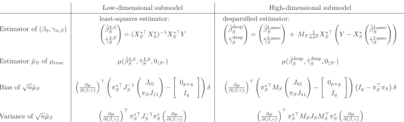
The results of last two sections for linear models are summarized in Table 1. We observe that the expressions giving the limiting variance of ˆµS are very similar. In the high-dimensional submodel case,

J_S−1 is not available and is thus replaced byMSJSMS. Regarding the bias, it is possible to show in both

cases that ifS0,n⊂Sthen the bias expression reduces to 0.

In practice, when computing the squared bias, we need to estimateδδ⊤_{. There are several possibilities}

to do it but none of them produces a consistent estimator. We list here four possibilities. A first natural choice is to use the Lasso estimator ˆδLasso₌√_n_γ_ˆLasso_where

( ˆβLasso,γˆLasso) = arg min

β,γ 1 2n Y −X ∗ β γ ! 2 2 +λ_kβ_k₁+λ_kγ_k₁. (14)

A second possibility is to use the more sophisticated adaptive Lasso ˆδadap ₌ √_n_γ_ˆadap _{(see Zou, 2006)}

where

( ˆβadap,γˆadap) = arg min

β,γ 1 2n Y −X ∗ β γ ! 2 2 +λ p X j=1 wjβj+λ p+q X j=p+1 wjγj. (15) withwj =    1 n−1/2₊_|βˆLasso j | for 1_≤j_≤p 1 n−1/2₊ |ˆγLasso j | forp+ 1≤j≤p+qn.

This can provide a better estimator ofδin view of asymptotic results of Zou (2006). A third possibility is to use the desparsified estimator of the full model ˆ

δdesp ₌√_n_ˆ_γdesp _{defined as}

ˆ βdesp ˆ γdesp ! = βˆ Lasso ˆ γLasso ! + M 1 nσ2X∗⊤ Y −X t βˆLasso ˆ γLasso !! ,

whereM is a relaxed inverse of the Fisher information matrixJ = 1

nσ2X∗⊤X∗obtained by the nodewise

regression technique. The fourth possibility follows from Lemma 3 applied to S = (1, . . . , qn). Under

suitable conditions we have ˆδdesp ₌.

d Nq(δ,Ω) +ˆ oP(1) where ˆΩ = (M JM)−p,−p is obtained by deleting

the firstprows and the firstpcolumns ofM JM. Thusδdesp_δdesp,⊤ _{has mean}_δδ⊤_{+ ˆ}_{Ω. This leads to a}

fourth possibility for estimatingδδ⊤_{: to use ˆ}_δdesp_δ_ˆdesp,t

−Ω. In case this quantity would be negative, itˆ can be truncated to zero. To summarize, we propose the four following ways to estimateδδ⊤ _{in the FIC}

formula: (1) ˆδLasso_(ˆ_δLasso₎⊤_{, (2) ˆ}_δadap_(ˆ_δadap₎⊤_{, (3) ˆ}_δdesp_(ˆ_δdesp₎⊤_{, (4) ˆ}_δdesp_(ˆ_δdesp₎⊤₋_Ω.ˆ

6 Simulation study

We perform a simulation study to illustrate the benefits of the high-dimensional FIC. We consider the linear modelYi=Xiγn+σǫǫi withǫi∼ N(0,1) fori= 1, . . . , n. We consider sample sizesn= 100 and

(15)

Low-dimensional submodel High-dimensional submodel Estimator of (β0, γn,S) least-squares estimator: ˆ βLS S ˆ γLS S ! = (X∗⊤ S XS∗)−1XS∗⊤Y desparsified estimator: ˆ βSdesp ˆ γ_Sdesp ! = βˆ Lasso S ˆ γLasso S ! +MSnσ12XS∗⊤ Y−XS∗ ˆ βLasso S ˆ γLasso S !!

Estimator ˆµSofµtrue µ( ˆβSLS,γˆSLS,0|Sc) µ( ˆβdesp_S ,γˆ_Sdesp,0_|_Sc)

Bias of√nµˆS ∂µ ∂(β,γ) ⊤ π∗⊤ S JS−1 J01 πSJ11 ! − " 0p×q Iq #! δ ∂µ ∂(β,γ) ⊤ π∗⊤ S MS J01 πSJ11 ! − " 0p×q Iq #! Iq−π⊤SπSδ Variance of√nµˆS ∂µ ∂(β,γ) ⊤ π∗⊤ S JS−1π∗S ∂µ ∂(β,γ) ∂µ ∂(β,γ) ⊤ π∗⊤ S MSJSMS⊤πS∗ ∂µ ∂(β,γ)

Table 1: Estimator ˆµSof the focus and its bias and variance for a low-dimensional and a high-dimensional

submodel in the context of a linear model.

n = 200 and two different possibilities for the dimension q of the paramater γn: q= 80 and q = 200.

The caseq= 200 corresponds to high-dimensional data for which the classical FIC can not be used. We generate the true model according to four scenarios:

• Case 1: γn = 10c(1,−1,1,−1,1,0, . . . ,0)/√nandXi fromNq(0, Iq) fori= 1, . . . , n.

• Case 2: γnas in case 1 andXifromNq(0,Σ) fori= 1, . . . , nwith Σjj = 1 and Σjk= 0.5 forj6=k.

• Case 3: γn = 10c(1,−1₂,1₃,−1₄, . . . ,±1_q)/√nandXi as in case 1

• Case 4: γn as in case 3 andXi as in case 2.

Cases 1 and 2 correspond to sparse models and cases 2 and 4 correspond to models with correlation between variables. The parameter ccontrols the amplitude of the components of γn. We consider three

different focuses. The first focus is the predictionµ1(γn) =X0γnfor a new valueX0of the covariate vector

with the components ofX0 randomly generated fromU[−1,1]. The second focus is the first coefficient

of γn, that is µ2(γn) =γn,1 and the third focus is the last coefficient ofγn, that isµ3(γn) =γn,q. Note

that the true value of the last focus is 0 for the sparse settings (cases 1 and 2).

We compare predictions of the focusµj for two types of methods: (i) we compute a penalized estimator

of γn in the full model and make prediction based on this parameter estimate and (ii) we use the

high-dimensional FIC as described in Sections 3 and 4. We consider two penalized estimators, the Lasso and the adaptive Lasso, with the tuning paramaters chosen by 10-fold cross-validation. Other tuning parameter choices are possible too. These two penalized estimators are also used to estimate δ in the FIC procedure. We thus obtain four different predictions of µj. For the estimation of σǫ2, we follow

the recommendation of Reid et al. (2016) and use ˆσ2

ǫ = RSS/(n−df) withb df the number of non-zerob

coefficients of the penalized estimator ofγn.

Because the number of covariates is large, it is computationally impossible to obtain the FIC of every possible submodel. Instead, we propose to use a backward-forward stepwise procedure with two possible starting sets: the empty set and the set _{j : ˆδj 6= 0} of active components of the estimator of δ. The

(16)

two procedures usually converge to two different subsets S1 and S2 and we keep the one that gives the

smallest FIC value. More refined procedures can be used to improve the selection search. It is for example possible to do some pseudo-exhaustive search by computing the FIC of all submodels upto a certain size

d.

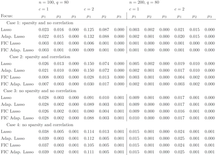
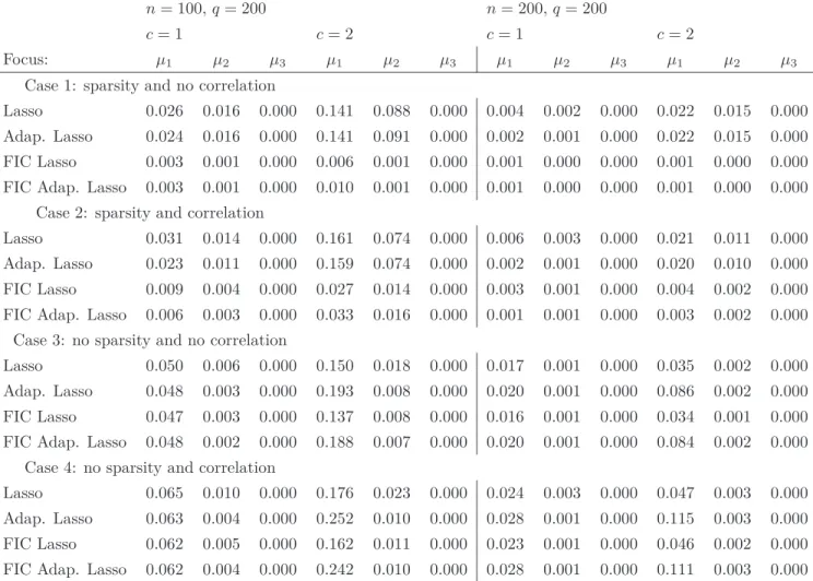
In Tables 2 to 4, we report the averaged squared errors of the estimators for the three different focuses over 1000 simulated datasets for different settings. In Table 2 we consider settings with 80 covariates and in Table 3 we increase the number of covariates to 200, obtaining high-dimensional data for which the traditional FIC could not be used. Results for these two tables are similar. We observe that all methods perform well for the third focusµ3=γq. Regarding focuses 1 and 2 we observe that the FIC procedures

outperform the penalized estimators for the sparse settings (cases 1 and 2), the ones that are supported by the theory. For non-sparse settings (cases 3 and 4), the different methods are equally competitive. The presence of correlation makes things slightly more complicated.

In Table 4, we compare the sensitivity of the different methods to the standard noise levelσǫ. We observe

that in the sparse cases, the FIC takes much more advantage of the decrease of the noise level. For

σǫ= 0.25 the FIC largely outperforms the penalized methods while for σǫ = 1 the methods are equally

competitive.

We conclude this simulation study by a remark on the size of the models selected by the FIC. We observed in our simulations that the models selected by the FIC procedure are very often of size smaller than 5. It turns out that it is often possible to find a small submodel S whose FIC is smaller than the FIC of

Strue, the active set of the model having generated the data. On Figure 1, we illustrate this by giving the

scatter plot of FIC(S) versus ˆµS for every possible submodel of size smaller or equal to 3. The setting is

chosen to have many true non-zero coefficients (20) so that we expect the bias to be large for models of size only 3. We also choose a small value of the standard noise (σǫ = 0.1) to increase the weight of the

squared bias in the FIC expression. We see on the left figure that many of the submodels exhibit large values of FIC but more importantly we also notice on the right figure that for some of the small models (about 3% of them), the FIC value is smaller than the FIC of the true model. For such submodels, the estimator ˆµS is very close to the true value (the grey horizontal line). This should be considered one of

the strong features of the FIC.

7 Real data example: the riboflavin data

We apply the high-dimensional FIC procedure on the riboflavin data that can be found in the R package

hdi (Meier et al., 2014). The data contains 71 observations, 4088 predictors (gene expressions) and a response variable measuring the riboflavin production of the Bacillus subtilis bacteria. This dataset has been used by many authors in the high-dimensional literature including van de Geer et al. (2014) and Javanmard and Montanari (2014). We center the response variable and randomly split the data into a training set (Xtrain, Ytrain) of size 50 and a testing set (Xtest, Ytest) of size 21. We then consider the

(17)

G u eu n in g a n d C la es k en s 1 6 n= 100,q= 80 n= 200,q= 80 c= 1 c= 2 c= 1 c= 2 Focus: µ1 µ2 µ3 µ1 µ2 µ3 µ1 µ2 µ3 µ1 µ2 µ3 Case 1: sparsity and no correlation

Lasso 0.023 0.016 0.000 0.125 0.087 0.000 0.003 0.002 0.000 0.021 0.015 0.000 Adap. Lasso 0.022 0.015 0.000 0.132 0.088 0.000 0.002 0.001 0.000 0.020 0.015 0.000 FIC Lasso 0.003 0.001 0.000 0.006 0.001 0.000 0.001 0.000 0.000 0.001 0.000 0.000 FIC Adap. Lasso 0.003 0.001 0.000 0.009 0.001 0.000 0.001 0.000 0.000 0.001 0.000 0.000

Case 2: sparsity and correlation

Case 3: no sparsity and no correlation

Case 4: no sparsity and correlation

Table 2: Averaged squared errors of the estimators for the three different focuses over 1000 simulated datasets and for different settings. µ1 is a random new observation, µ2 =γ1 and µ3 =γq. The number of covariates is q = 80, the standard noise is σǫ = 0.25 and c is a parameter controlling the amplitude of the components ofγn.

(18)

G u eu n in g a n d C la es k en s 1 7 n= 100,q= 200 n= 200,q= 200 c= 1 c= 2 c= 1 c= 2 Focus: µ1 µ2 µ3 µ1 µ2 µ3 µ1 µ2 µ3 µ1 µ2 µ3 Case 1: sparsity and no correlation

Table 3: Averaged squared errors of the estimators for the three different focuses over 1000 simulated datasets and for different settings. µ1 is a random new observation, µ2=γ1 and µ3 =γq. The number of covariates is q= 200, the standard noise is σǫ = 0.25 and c is a parameter controlling the amplitude of the components ofγn.

(19)

Focus: µ1 µ2 µ3

Standard noise: σǫ 1 0.5 0.25 1 0.5 0.25 1 0.5 0.25

Case 1: sparsity and no correlation

Lasso 0.086 0.024 0.023 0.036 0.013 0.016 0.001 0.000 0.000 Adap. Lasso 0.060 0.015 0.022 0.014 0.007 0.015 0.001 0.000 0.000 FIC Lasso 0.063 0.013 0.003 0.013 0.003 0.001 0.002 0.000 0.000 FIC Adap. Lasso 0.063 0.011 0.003 0.012 0.003 0.001 0.002 0.000 0.000

Lasso 0.188 0.086 0.038 0.084 0.018 0.005 0.002 0.001 0.001 Adap. Lasso 0.204 0.088 0.039 0.035 0.008 0.003 0.003 0.001 0.001 FIC Lasso 0.195 0.085 0.037 0.045 0.011 0.003 0.003 0.001 0.001 FIC Adap. Lasso 0.223 0.091 0.039 0.034 0.008 0.002 0.005 0.002 0.001 Table 4: Averaged squared errors of the estimators for the three different focuses over 1000 simulated datasets and for different settings. µ1is a random new observation,µ2=γ1andµ3=γq. Parameters are

q= 80,n= 100 and c= 1. Results are given for different values of the standard noise: σǫ= 1,0.5,0.25.

In a first step we compute a Lasso estimator ˆβLasso _of _β _{with the tuning paramaters chosen by}

10-fold cross-validation and we obtain estimators ˆµLasso

j =X

j

testβˆLasso of the 21 focuses. In a second step

we apply our FIC procedure. For each of the 21 focuses, we search for a submodel that provides a small FIC value. As in the simulation study, we apply a backward-forward stepwise procedure with two possible starting sets: the empty set and the set selected by the Lasso. We denote by S1j and S

j 2

the sets obtained for the focus j with these two choices of starting sets. We then keep the best of the two by definingSj _{= arg min}

S∈{Sj1,S

j

2}FICj(S). We compute the corresponding estimator ˆβS

j and

obtain an estimator ˆµFIC j =X

j

testβˆSj of the focus µ_j. We then compute the mean squared prediction

errors 1/21P21j=1(Y j

test−µˆj)2 for ˆµj = ˆµLassoj and ˆµj = ˆµFICj . For comparison purpose, we also compute

estimators of the focuses with S1j and S j

2. Note that each computation of the FIC takes about one

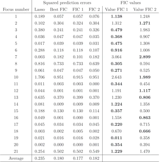
millisecond on a regular computer. Thus, each step of the stepwise procedure takes about four seconds. The results are reported in Table 5. We observe that the three strategies for performing the FIC op-timization are very competitive and all outperform the Lasso (0.180, 0.177 and 0.182 versus 0.235 for

(20)

Gueuning and Claeskens 19 0 500 1000 1500 −2 0 2 4 FIC(S) m u(S) 0.00 0.05 0.10 0.15 0.20 0.40 0.45 0.50 0.55 0.60 FIC(S) m u(S)

Figure 1: Parameters: n= 100,q= 80,p= 0,s0 = 20,σǫ = 0.1,c= 1,µ1. Scatterplots of ˆµ(S) versus

FIC(S) for all the 85401 possible models of size smaller or equal to 3. The true δ and the trueσǫ are

used in the FIC computations. The red triangle corresponds to the true model of size 20 and the blue square corresponds to the model minimizing the FIC amongst the models of size smaller than 3. The right figure is a zoom of the left figure.

the Lasso). We also observe that for two third of the focuses (14 out of 21), the set S1 was chosen,

corresponding to work with the empty set as starting set. In Table 6, we report information about the variables selected by the different procedures. As expected, the setSj₁is generally smaller (4.7) than the setS2j(10.7). Furthermore, we note that only two variables are selected at least three times by FIC 1 and

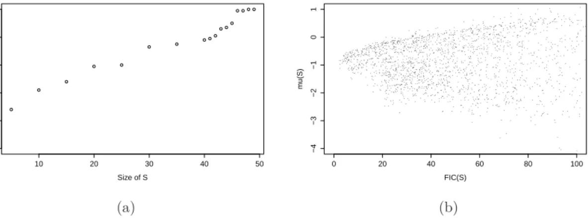
none of them is also selected by the Lasso. Conversely, all the 10 variables selected at least three times by FIC 2 are also selected by the Lasso. To conclude, we observe that the FIC uses for each prediction much fewer variables than the Lasso (6.7 versus 27) but in total the number of different variables used by the FIC for the 21 predictions is much larger than for the Lasso (120 versus 27). This is a key feature of the FIC. 10 20 30 40 50 0 20 40 60 80 100 Size of S 0 20 40 60 80 100 −4 −3 −2 −1 0 1 FIC(S) m u(S) (a) (b)

Figure 2: (a) For different subset sizes, the number of times that the desparsified FIC of Section 4 is smaller than the OLS FIC of Section 3 for 100 random subsets and for the first focus. (b) Scatterplot of ˆ

(21)

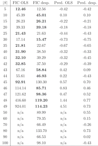
We end this section by numerically comparing the behaviour of the low-dimensional FIC (OLS) introduced in Section 3 to the high-dimensional FIC (desparsified) presented in Section 4. Summary of the formulas can be found back in Table 1. We refer to these two FIC as OLS FIC and desparsified FIC. We consider the first focusµ1=Xtest1 βof the real data example and compute the two FIC values for different subsets.

Note that these two FIC aim at estimating the mean squared error of two different estimators (see Table 1). More concretely, we consider subsets of the 4088 covariates of size going from 5 to 49. Recall that the training sample size is 50. For each of the considered sizes we consider 100 different subsets.

In Table 7 we give the two FIC values and the two predictions for the first considered subset of each size. Note that the true value of the focus is unknown but we can expect it to be close to y1

test =−1.13. We

see that for small subsets the results are very close to each other. When_|S_|increases,MS gets further

away fromJS−1so that the estimators become more and more different. When |S|is close to the sample

size 50 the quality of the OLS estimator deteriorates and it is better to use the desparsified estimator. In Figure 2(a) we count how many times out of 100 random choices of the subsets the desparsified FIC is smaller than the OLS FIC. We observe that from size 20 the desparsified FIC tends to outperfom the OLS FIC. This gets more and more pronounced when _|S_| gets closer to the sample size. In any case for each S we can always compute both FIC and keep the smaller one. Recall that they refer to different estimators. In Figure 2(b), we give the scatterplot of FIC(S) versus ˆµS for 2300 submodels

of size 5,10, . . . ,40,41, . . . ,49,50,60, . . . ,100 (100 submodels of each size). We observe that the FIC obtained with the desparsified procedure behaves as it is supposed to: the FIC aims at estimating the expected value of 50(ˆµS−µtrue)2 and we do observe a quadratic shape, which is slightly altered due to

the difficulty to estimateδin this high-dimensional example.

8 Extensions and discussion

8.1 Focused selection for high-dimensional generalized linear models

The results of Section 4 can be extended to high-dimensional generalized linear models (GLM). Let us consider observations Y1, . . . , Yn where Yi has density f(y, Xi, θ0, γ0+δ/√n) fori = 1, . . . , n with f

from the exponential family of distributions. Consider a high-dimensional submodel S containing the true active set S0,n Let us write βS =

θ γS

!

and denote the loss function for an observation (y, x) by ρβS(y, x) = −logf(y, x, θ, γS, γ0,Sc). We define the first an second partial derivatives of the loss

function as ˙ρβS =

∂

∂βSρβS and ¨ρβS =

∂2

∂βS∂β_S⊤ρβS and use the following notation: for a functiongwe write Png=_n1Pn_i=1g(Yi, Xi). We use the penalized estimator

ˆ θL S ˆ γL S ! = ˆβLS = arg min βS=(θ,γS) PnρβS +λkβSk1.

Similarly to van de Geer et al. (2014), we define ˆΣS =Pnρ¨_βˆL

S and ˆMS as a relaxed inverse of ˆΣS obtained

(22)

(ˆθL

S,γˆSL, γ0,Sc). We define the following desparsified estimator

ˆ θdesp_S ˆ γSdesp ! = θˆ L S ˆ γSL ! −MˆSPnρ˙_θˆL S,ˆγLS. (16)

Using results from van de Geer et al. (2014), we can show that ˆ θ_Sdesp₋θ0 ˆ γSdesp−γ0,S ! = 0 δS ! −MˆSPnρ˙βˆtrue S +oP(n −1/2₎ ₍₁₇₎ and that ˆMSPnρ˙_βˆL Sρ˙ ⊤ ˆ βL S ˆ M⊤

S is a consistent estimator of the variance of√n(ˆθ desp,t

S −θ⊤0,γˆ desp,t

S −γ0,S⊤ )⊤.

This leads to a result similar to Theorem 2 whereMSJSMS is replaced by ˆMSPnρ˙_βˆL Sρ˙ ⊤ ˆ βL S ˆ M⊤ S.

8.2 Model averaging in high-dimensional models

Averaging estimators across several good models is another interesting route, also in the high-dimensional setting. Since estimators in a selected model can be written as model averaged estimators assigning weight one to the estimator in the selected model, and weight zero to all other models, the tool of model averaging is important to study proper post-selection inference.

Let the weighted estimator be obtained in the following way ˆ

µavg=

X

S∈A

wS(ˆδ)ˆµS,

where ˆµS =µ(ˆθS,ˆγS, γ0,Sc) and Ais the set of models under consideration for averaging, this does not

need to be the set of all possible submodels of the largest available model. The weight for eachS, may be deterministic, e.g., assigning equal weight to each of the models, or a predetermined weight that is not data-dependent, or the weights may be data-driven, e.g.,wS(ˆδ) =I{S= arg minS′_∈AFIC(S′,δˆ)} in

the FIC selection case.

Using Lemma 3, or equation (17) in the GLM case, we obtain that the desparsified estimator ˆδdesp ₌. d

˜

δ∼ Nq(δ,Ω). Using the joint convergence of the random weightswS(ˆδ) and√n(ˆµS−µtrue) forS ∈ Ato

their respective limits, we obtain the following Corollary to Theorem 2.

Corollary 1. Assume the local misspecification setting. Under the assumptions of Theorem 2, for a set of weights such that P_S_∈AwS(d) = 1 for alldand with at most a countable number of discontinuities,

√ n ( X S∈A wS(ˆδ)ˆµS−µtrue ) →dΛavg= X S∈A wS(˜δ)ΛS.

The limiting variable is in case of deterministic weights again normal. For random weights the limit distribution is a sum of products of the random weights and the normal limits ΛS, which is in general

not longer normally distributed. The mean of the limit random variable depends on the random weights

wS(˜δ) and its correlation with the random variables CS, DS,

E(Λavg) =− ∂µ ∂γ ⊤ δ+X S∈A E " wS(˜δ) ( ∂µ ∂θ ⊤ CS+ ∂µ ∂γS ⊤ DS )# .