Study of Flow Behavior of Ultrafine Particles
Agglomerations in the Riser
J. Zheng1∗, X. Zhu2, Y. Wang1, Ch. Xu1
1- School of Energy and Power Engineering, Northeast Dianli University, Jilin 132012, China 2- School of Science, Northeast Dianli University, Jilin 132012, China
Abstract
Flow behavior of gas and agglomerates is numerically investigated in the riser based on a transient two-fluid model. The gas phase is modeled by the LES model, and the solid phase uses a kinetic theory model developed from the molecular model coupling the gas-agglomerates interaction and the agglomerates-agglomerates interaction[1]. We assumed that the ultrafine particles move as natural agglomerates rather than single particles in the riser. The energy transfer and dissipation by the instantaneous collisions between the agglomerates of ultrafine particles and gas phase and between agglomerates-agglomerates are considered. The diameter of agglomerates is estimated based on the force model by Li and Tong[2].The distributions of velocity, concentration and diameter of agglomerates, are numerically obtained. The influence of flow and agglomerates in the different operating conditions is also analyzed. The results show that the large agglomerates are rich in the bottom section of the bed. Thus the Fast Fourier Tranform (FFT) is used to get the fluctuated character of the agglomerates in the riser and find the dominant frequency of the agglomerates fluctuation is 0.03-1.26Hz.
Keywords: Ultrafine Particles; Agglomerates; Force Balance Method; Numerical
Simulation, Power Spectrum Density
∗ Corresponding author: [email protected]
1. Introduction
Ultrafine particles are in the Geldart-C group (cohesive powders) [3]. They have many attractive properties to industrial applications since these powders have advantages of high reaction rates and uniform microstructures, but are easily agglomerated. Many researchers investigated the fluidization behavior of ultrafine particles by experiments[4-6]. The flow behavior of
bed. Liu[9] and Zeng[10] study the flow behavior of ultrafine particles mixture in the magnetic fluidized beds. Liu[9] found the flow behavior of mixture of cohesive particles in the combine of sonic fluidized bed and magnetic fluidized bed.
Experiments observed that the ultrafine particles will exist in a state of natural agglomerates and a state of fluidized agglomerates in a fluidized bed. About the agglomerates of ultrafine particles, the pioneer researchers observed and estimated the growth and break between the ultrafine particles-the ultrafine particles or agglomerates-agglomerates. Li et al. [2]studied the size of agglomerates in the riser by the method of force balance. Xu and Zhu[11] estimated the diameter of the agglomerates in the fluidized bed based on the energy balance.
Regarding the simulation of the flow behavior of the ultrafine particles, a few works have been done. Helland et al. [12] simulated the flow structure of cohesive powders in a riser based on an Eulerian– Lagrangian approach. Jung et al. [13] used the two-fluid model with results from the kinetic theory of granular flow coupled with an empirical cohesive force model to simulate the fluidizing structures of cohesive particles in bubbling fluidized beds. Sunun et al. [14] simulated the flow behavior of the different size cohesive particles in the vibration fluidized bed based on the Lagrangian model. Saiki et al. [15] simulate the flow behavior of cohesive particles in a fluidized bed by DEM Coarse Grain Model. In this work, the flow behavior of gas and agglomerates is simulated by transient two-fluid model. The gas model is based on the
LES model, the agglomerates model is modified from the molecular model and the model proposed by Arastoopour et al [1]. We use the natural agglomerates as the single ultrafine particles in the simulation of flow in the riser. Then the diameter of the fluidized agglomerates in the flow is estimated by the force balance model proposed by Li [2]. The simulation results are compared with experimental data of Li [2]. The distribution of velocity and concentration of agglomerates are numerically obtained. The effect of operating condition and the Power Spectrum Density are analyzed.
2. A gas-agglomerates two-fluid model with agglomerate-based approach
Ultrafine particles belong to Geldart C particles. Two or more ultrafine particles can be agglomerated by the action of collision. The agglomerate is a group of ultrafine particles bonded together and moving with the same velocity. Arastoopour et al[1] developed constitutive equations for fluidizations of ultrafine particles by considering the action of collision through introducing the contact bonding energy Ec which will impact the growth of the agglomerates in the fluidization of ultrafine particles. The fluctuation energy of the granular temperature of particles is also related to the collision of agglomerates-agglomerates. To establish the transient two-phase fluidized model for the flow of gas and agglomerates phases, the following assumption is set: (1), the particles are sphere; (2) the porosity of the agglomerates is assumed to be equal to the zero, εa=0. That
The gas flux through the agglomerates is neglected, and the influences of the gas velocity to particles agglomerates are ignored. The concentration of gas phase εg
and the concentration of agglomerates εs is
equal to εs+εg +εa≈εs+εg=1.
2-1. Conservation of mass for gas and agglomerates phases
The mass balance equation of gas phase is expressed as follows:
0 ) (
)
( g g +∇⋅ g gug = t G ε ρ ε ρ ∂ ∂ (1)
For agglomerates phase, the mass balance equation is:
(
)
+∇⋅(
)
=0 ∂ ∂ s s s s s u t G ρ ε ερ (2)
2-2. Momentum equations of gas and agglomerates phases
The momentum balance for the gas phase is given by the Navier–Stokes equation, modified to include an interphase momentum transfer term ) ( ) ( ) ( s g g g g g g g g g g g g u u p u u u t G G G G G − − + ⋅ ∇ + ∇ − = ⋅ ∇ + β ρ ε τ ε ρ ε ρ ε ∂ ∂ g (3)
where τg is the viscous stress tensor of gas phase: g g g T g g g g
g u u u
G G G ⋅ ∇ − ∇ + ∇ =ε μ ε μ τ 3 2 ]
[ (4)
The effective viscosity of gas phase μg is the
sum of dynamic viscosity μg,l and turbulent
viscosityμg,t. The gas phase turbulence is modeled by the Sub Grid Scale (SGS) model, and thus the gas turbulent viscosity can be estimated as[16] :
) : ( ) 1 . 0 ( 2
,l g g g
g
g μ ρ τ τ
μ = + Δ (5)
3 / 1
) (ΔxΔyΔz
=
Δ (6)
For agglomerates phase, the momentum balance equation is
(
)
(
)
(
)
) ( g s
s s c k s s s s s s s u u g T T u u u t G G G G G G − + + + ⋅ −∇ = ⋅ ∇ + ∂ ∂ β ρ ε ρ ε ρ ε (7) where β is the Drag force coefficients of gas–
agglomerates. Because we focus on agglomerate contribution to flows, the particle diameter used in the original formulations of the kinetic theory of cohesive particles flow in Arastoopour et al[1] is replaced by the agglomerate diameterσ . The diameter of agglomeratesσ is established by the force balance method proposed by Li[2]. The solid pressure Ps and the shear viscosity
μs represent the normal force by
particle-particle interaction. For agglomerates the additional term ξp
( )
Rc and ξv( )
Rc are added to account for the momentum exchange between agglomerates.Where using the dynamics force Tk and collision force Tk we get,
I
Tk =εsρsθgran (8)
(
)
⎥⎦⎤⎢⎣
⎡ + ∇⋅ −
= p I S u I
Tc s s s Gs
6 5
2ε μ 0 (9)
(
ij ji)
(
s)
ijij W W u
S = + − ∇⋅G δ
3 1 2
( )
(
p c)
s
s p R
p = 0 1+ξ (11)
( )
(
v c)
s
s μ ξ R
μ = 0 1+ (12)
gran c c m e E R θ 2
= (13)
(
1)
1 )
( 2 −
+
= −Rc
c
p e
e e R
ξ (14)
⎥ ⎦ ⎤ − + ⎟ ⎠ ⎞ ⎜ ⎝ ⎛ + − + ⎢ ⎢ ⎣ ⎡ ⎟⎟ ⎠ ⎞ ⎜⎜ ⎝ ⎛ − + ⎟⎟ ⎠ ⎞ ⎜⎜ ⎝ ⎛ − + + = − 1 8 8 1 32 32 ln 16 4 32 2 1 1 ) ( 4 6 8 6 4 4 2 2 c c c c c c c c R c v R R R R R R R R e e e R c γ γ ξ (15)
(
)
s s grans e g
p ε ρ 0θ
2
0 =21+ (16)
(
)
π θ σ ρ ε μ gran s ss = g 1+e
5 4
0
0 (17)
2-3. Conservation of the fluctuating energy The conservation equation of fluctuating energy of agglomerates can be expressed:
(
)
(
)
(
f C)
mC N u T T q q u t drag s s c s c k c k gran s s s gran s s K G G G G G G G ⋅ + ⎟ ⎠ ⎞ ⎜ ⎝ ⎛ + ∇ + − + ⋅ −∇ = ⎥ ⎥ ⎦ ⎤ ⎢ ⎢ ⎣ ⎡ ⎟⎟ ⎠ ⎞ ⎜⎜ ⎝ ⎛ ⋅ ∇ + ⎥ ⎥ ⎦ ⎤ ⎢ ⎢ ⎣ ⎡ ⎟⎟ ⎠ ⎞ ⎜⎜ ⎝ ⎛ ∂ ∂ ρ ε θ ρ ε θ ρ ε 2 2 1 : 2 3 2 3 (18) ⎟⎟ ⎠ ⎞ ⎜⎜ ⎝ ⎛ = 2 2 C C
qGk εsρs K (19)
2
1 c
c
c q q
q = + (20)
⎭ ⎬ ⎫ ⎥ ⎦ ⎤ − ⎟ ⎠ ⎞ ⎜ ⎝ ⎛ + + − ⎟ ⎠ ⎞ ⎜ ⎝ ⎛ − + ⎟ ⎠ ⎞ + − ⎩ ⎨ ⎧ ⎢ ⎣ ⎡ ⎜ ⎝ ⎛ + + − = − 10 8 6 6 8 6 4 2 0 1 448 3 448 3 56 1 56 ln 28 1 224 3 448 3 28 1 7 1 1 1 3 224 2 c c c c c c c c c R gran s s s c R R R R R R R R R e e g q c γ γ π θ ε ρ ε (21)
(
)
[
]
⎪⎭ ⎪ ⎬ ⎫ ⎥ ⎦ ⎤ ⎥ ⎦ ⎤ − ⎟ ⎠ ⎞ ⎜ ⎝ ⎛ − + + ⎟ ⎠ ⎞ ⎜ ⎝ ⎛ + + ⎟ ⎠ ⎞ + − ⎢ ⎣ ⎡ ⎜ ⎝ ⎛ + + ⎩ ⎨ ⎧ ⎢⎣ ⎡ + ⋅ ∇ + + − = − − 10 8 6 8 6 6 4 2 0 2 256 3 32 1 256 3 32 ln 128 3 16 1 256 3 16 1 4 1 1 15 2 10 1 7 30 1 15 14 2 2 c c c c c c c c c R R s ji ij gran s s s c R R R R R R R R R e e e I u W W g q c c γ γ π π π θ σ ε ρ ε G (22)2-4. Drag force coefficients of gas– agglomerates
fluidized beds. Yu Wen gs gs Ergun gs
gsβ (1 ϕ )β &
ϕ
β = + −
(23)
2
2 2
150 s g 1 75 s g g s 0 8
gs Ergun g
g g u u . ε ρ . ε μ β ε ε σ ε σ − = + ≤ G G (24) 8 . 0 4
3 2.65
& > − = − g g s g g s d Yu Wen gs u u C ε ε σ ρ ε β G G (25)
(
)
[
150 1.75 0.2]
0.5arctan × − +
=
π
ε
ϕ s
gs (26)
Re / ) Re 15 . 0 1 (
24 + 0.687
=
d
C Re≤1000 (27)
44 . 0 =
d
C Re>1000 (28)
g s g g
gε σ u u μ
ρ /
Re= G − G
(29)
Note that the drag force exerted on solids in the present model is based on a phenomenological consideration (i.e., agglomerating of particles). Therefore, a more appropriate correlation for drag coefficient would improve the performance of the model.
2-5. Equivalent diameter of agglomerates
The agglomerated size predicted models can be classified into two types: the force balances [2, 19] and the energy balances [4, 20, 21] In the present model, we estimated the diameter of agglomerates σ by the force balances model. The detailed assumption is described in the paper of Li[2].
0 4 ] ) ( 3986 . 0 33 . 0 [ ) ( 2 5 / 1 2 3 6 8 . 2 2 2 = + + − − − πδ σ ρ ε ρ σ ρ ρ A k V u g a a g g g g a G (30)
2-6. Initial and boundary conditions
For gas phase, the surface of the wall adapts without sliding boundary condition. Wall particle velocity and temperature adapts the equations listed below:
(
)
1 2 1 3 3 0 6 1k f sl f
s s s
sl
' /
s s sl / s ,max s s ,max
v
n.( ). ( n. .n ) tan
\v \ v / σ σ σ δ φ πρ ε θ ε ε ε + + + = ⎡ − ⎤ ⎣ ⎦ (31)
(
)
(
)
(
)
(
)
1 2 2
1 3
3 2 2
1 3 3 6 1 3 1 4 1 ' /
s s sl
s /
s ,m ax s s ,m ax
/
s s w
/ s ,m ax s s ,m ax
v k / e / φ πρ ε θ θ ε ε ε πε ρ θ ε ε ε ⋅ ∇ = ⎡ − ⎤ ⎣ ⎦ − − ⎡ − ⎤ ⎣ ⎦ n (32)
Where n is the unit normal vector from the boundary to particle group; δ is material fiction angle, φ' is the mirror reflection
factor, the value is 0.5 in the simulation; ew is elasticity recovery factor, vsl is particle
sliding velocity, namely the difference between the particle group velocity and the wall velocity, vsl = vs −vwall
3. Results and discussion
The simulation properties were based on the measured result of the Li and Tong’s [2]experiments. The ultrafine particles we used are calcium carbonate (CaCO3). The
gas-particles properties and the other information needed in the simulation are listed Table 1.
Fig. 1 shows comparisons of the simulated concentrations of agglomerates with experimental data of Li and Tong[2] at two superficial gas velocities of 1.89m/s and 2.52m/s, respectively. Both computed and experimental concentration profiles show the concentration of agglomerates is high in the bottom of the riser. With a rise in the height, the concentration of agglomerates decrease. In the experiment, the particles are recovered into the riser at one-side inlet from V-valve, while gas and particles are fed to the system from the bottom in the numerical simulations. This causes the differences in the flow patterns and pressure drop in the bottom of the riser. Then, the discrepancies between the simulated and measured result are noticed.
Table 1. Parameters for simulations.
Hamaker Constant A 1.198x10⁻¹⁹J
Inlet Particle Concentration 0.15
Inlet Gas Velocity 1.89m/s
Temperature T 300 K
Height of Riser H 3.25 m
Diameter of Riser 2R 0.075 m
Mesh 26X158
Constant Time Step Δt 10-5s
Total Simulation Time 50s
Particle Shape sphere
Particle Size d 4.3μm
Density of Particles ρs 2200 kg/m3
Bulk Density of Particles ρb 539 kg/m3
Restitution Coefficient ew 0.5
Restitution Coefficient e 0.5
Contacting Bonding Energy Ec 3.0x10⁻¹⁵ kgm2/s2
0.00 0.02 0.04 0.06 0.08 0.10 0.12
0 50 100 150 200 250 300 350
Height,cm
Concnetration of agglomerates
ug=1.89m/s-H. Li,H.Tong ug=2.52m/s-H. Li,H.Tong ug=1.89m/s-Simulation ug=2.52m/s-Simulation Gs=3.15kg.m3/s
Figure 1. Profile of concentration of agglomerates in the riser.
0.00 0.02 0.04 0.06 0.08 0.10 0.12 0.14 0.16
0 50 100 150 200 250 300 350
He
ight,cm
Diameter of agglomerates, cm
ug=1.58m/s, H, Tong and H, Li(2009)
ug=2.21m/s, H, Tong and H, Li(2009)
ug=1.58m/s, Simulation
ug=2.21m/s, Simulation
Gs=3.15kg.m3/s
CaCO3: d=4.3μm, ρs=2539kg/m3 ρ
b=2539kg/m
3
Figure 2. Profile of diameter of agglomerates in the
riser.
Fig. 2. illustrates the diameter of CaCO3
agglomerates is effected by the combined action of velocity and the concentration.
0.0036 0.0035 0.0033 0.0031 0.0029 0.0027 0.0025 0.0023 0.0021 0.0019 0.0017 0.0015 0.0013 0.0012 0.0010 0.0008 0.0006 0.0004 0.0002 0.0000
Figure 3. Computed instantaneous concentrations of
particle agglomerates.
Figure 4. Computed instantaneous velocity of the
particle agglomerates.
Fig. 3 and Fig. 4 illustrate the computed instantaneous concentrations and the computed instantaneous solid velocity of agglomerates at the times of 20.0, 30.0, 40.0 and 50.0 seconds at the superficial velocity and particle mass flux of 1.89 m/s and 3.15kg/m2s, respectively. The flow of agglomerates forms the annulus-core flow construct. The agglomerates in the riser center flow up and the agglomerates near the riser wall flow down. Near the riser bottom agglomerates tend to accumulate and then become dilute near the top of the riser, also more agglomerates are found near the wall of
the riser. Although the max concentration of the agglomerates in the riser shown in Fig. 1. is less than 0.004, the distribution of agglomerates is averaged relatively.
-0.4 -0.2 0.0 0.2 0.4
0.000 0.005 0.010 0.015 0.020 0.025 0.030 0.035 0.040
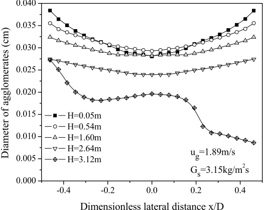
H=0.05m H=0.54m H=1.60m H=2.64m H=3.12m
ug=1.89m/s
Gs=3.15kg/m2s
Dia
m
eter
of agglomera
tes (cm)
Dimensionless lateral distance x/D
Figure 5. Time-averaged radial distribution of
agglomerates diameter in different height.
Fig.5. illustrates the radial distribution of agglomerates diameter in different height at the superficial velocity of 1.89m/s and the mass flux of 3.15kg/m2s. The diameter of agglomerates is low in the center and high near the wall. Along the height of the riser the diameter of agglomerates decreases but the size becomes average. Further, in the location of the outlet (H=3.12m, we set the outlet on the left wall), the diameter of agglomerates in the left is higher than in the right, as H=3.12m is located in the outlet. The direction of outlet turns left. The gas velocity changes to slow for the direction of velocity and the concentration of agglomerates in this location is rich. The collision between the ultrafine particles is frequent and easy to agglomerate. So the diameter of agglomerates to the left of H=3.12m is bigger than the right.
agglomerates as a function of superficial velocity. The agglomerates with a larger size appear near the wall in the riser for the function of gravity, buoyancy and drag and collision. With the comprehensive influence of this force balance, the lower gas velocity and the richer volume fraction of agglomerates near the wall the size of agglomerates is small near the section of the wall. However, the function of gravity is shown to be more important near the location of the wall. The size of agglomerates increases with the function of gravity force near the location of the wall. But in the center of the riser, agglomerates break for the function of shear force. So the diameter of agglomerates is smaller in the center than near the wall. With the increase of superficial velocity, the size of agglomerates decreases. The agglomerates are broken easily as a function of the shear force.
-0.4 -0.2 0.0 0.2 0.4
0.026 0.028 0.030 0.032 0.034 0.036 0.038
D
iameter
o
f ag
gl
om
er
ates,cm
Dimensionless lateral Distance, x/D ug=1.57m/s
ug=1.89m/s ug=2.20m/s ug=2.52m/s Gs=3.15kg/m3/s H=160cm
Figure 6. Time-averaged radial distribution of
agglomerate diameter as a function of superficial velocity.
Fig. 7. illustrates the radial distribution of agglomerates diameter in the different mass
flux of 1.229kg/m2s, 2.776kg/m2s and 3.15kg/m2s. The agglomerates diameter increases with the increase of the mass flux in the condition of the same gas velocity. With the increase of the mass flux, agglomerates grow up because more ultrafine particles collide and stick, and the size difference increases between the center and near the wall with this increase. More large agglomerates appear and pile up in the bottom and near the wall.
-0.4 -0.2 0.0 0.2 0.4
0.026 0.028 0.030 0.032 0.034 0.036
D
iame
ter
of
a
gglome
rates,
cm
Dimensionless Diatance, x/D Gs=1.229kg/m3/s Gs=2.776kg/m3/s Gs=3.15kg/m3/s ug=1.89m/s H=160cm
Figure 7. Time-averaged radial distribution of
agglomerates.
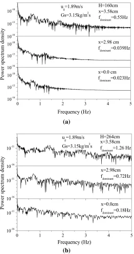
A better interpretation of a transient signal is possible by expressing the signal in the frequency domain which is obtained through the power spectrum density. The power spectrum indicates how the energy is distributed over the frequencies and provides more detailed information on the gas–solid flow process in the measured points[22]. Fig. 8 illustrates the power spectrum density (PSD) of instantaneous agglomerates concentration at the height of H=1.6m and H=2.64m. The result of the power spectrum density is based on the Fast Fourier transform (FFT) method. It can be seen that the PSD of the local instantaneous
0 1 2 3 4 5 10-16
10-13 10-10 10-16
10-13 10-10
10-16
10-13
10-10
x=0.0 cm fdominant=0.023Hz
Frequency (Hz)
x=2.98 cm fdominant=0.039Hz
Pow
er spectrum
den
sity
H=160cm x=3.58cm fdominant=0.55Hz
ug=1.89m/s
Gs=3.15kg/m2s
(a)
0 1 2 3 4 5
10-16 10-11 10-16 10-11
10-16 10-11
ug=1.89m/s
Gs=3.15kg/m2s
x=0.0cm fdominant=0.18Hz
H=264cm
Frequency (Hz)
x=3.58cm fdominant=1.26 Hz
x=2.98cm fdominant=0.72Hz
Powe
r spe
ct
rum densi
ty
(b)
Figure 8. Power spectrum density of instantaneous
concentration of agglomerates.
agglomerates concentration fluctuation exhibits a broad-band character with many spikes over a wide frequency range. The higher exchange of momentum and energy between the gas and agglomerates occurs at the location of x=3.58cm compared to the profile of PSD at the center. With the increase of frequency, the PSD decreases slowly. Compared with Fig. 8(a) and 8(b), the collision is more frequent in the location of x=3.58cm (near the wall). The value of PSD is bigger in the section of H= 160cm but
in the section of H=264cm, the value of PSD is relatively average for the lower concentration of agglomerates. The dominant frequency of the fluctuation emerges from 0.03 to 1.26. So fluctuation of the agglomerates is the low frequency ripple.
4. Conclusions
Based on the hydrodynamic theory of dense gas-solid flow and the kinetic theory of dense gases, the kinetic theory of cohesive particles flow and constitutive equations of cohesive particles are established. The energy transfer and dissipation by the instantaneous collisions between the agglomerates of cohesive particles and gas phase or between agglomerates-agglomerates are considered. The shear viscosity, pressure and collisional granular heat flux of agglomerates are derived. Thus, the kinetic theory of cohesive particles flow is proposed.
Under the principle of force balance, the collision of the agglomerates is considered as the collision interactions between two agglomerates. Whether the agglomerates will separate or not after collision is decided by the balance of the drag force, collision force, cohesive force, gravity and buoyancy force acting on the agglomerate. Thus the model of agglomerate size estimation is proposed, and used in the simulations.
core-annular flow structure was observed. The calculated result of agglomerate size shows that the large agglomerates favor the bed bottom and walls. In the outlet regime, the exit factor leads to the accumulation of agglomerates. Different operating conditions will directly influence the form and breakage of agglomerates because of the change of the collision force and other external forces. This will also affect the overall flow in the riser. Fast Fourier Transform (FFT) of instantaneous concentration shows that the dominant frequency of the particle fluctuation is 0.03-1.26Hz.
Acknowlegdments
This work is supported by the Science and Technology Developing Project of Jilin Province, China through Grant no. 201101109. We also appreciate the referees for their useful comments and help in improving the clarity of this manuscript.
Nomenclature
A Hamaker constant
D diameter of riser
e restitution coefficient of particles
ew restitution coefficient of particle and
wall
Ec contact bonding energy
F force
g gravity
g0 radial distribution function
Gs solid massflux
H height
I unit tensor
k function of Poisson’s ratio and Young’s modulus
n normal direction
P fluid pressure
Ps particle pressure Re Reynolds number
T time
ug gas velocity us particle velocity
x transverse distance from axis
z vertical distance
Greek letters
β drag coefficient
γ collisional energy dissipation εa porosity in the agglomerates
εg porosity of gas phase
εs concentration of agglomerates
εs;max maximum concentration of solids
θ granular temperature μg gas viscosity
μg,l dynamic viscosity of gas phase
μg,t turbulent viscosity of gas phase
μs shear viscosity
ρa density of agglomerate
ρs particle density
ρg gas density
σ diameter of agglomerate τg gas stress tensor
τs particle stress tensor
References
[1] Arastoopour, H., "Numerical simulation and experimental analysis of gas/ solid flow systems: 1999 Fluor-Daniel Plenary lecture", Powder Technology, 119, 59, (2001).
[2] Li, H. and Tong, H., "Multi-scale fluidization of ultrafine powders in a fast-bed- riser/conical dip leg CFB loop", Chemical Engineering Science, 59, 1897, (2004).
[4] Chauoki, J., Chavarie, C., Klvana, D. and Pajonk, G., "Effect of interparticle force on the hydrodynamic behavior of
fluidized aerogels", Powder Technology, 43, 117, (1985).
[5] Pacek, A. W. and Nienow, A. W., "Fluidization of fine and very dense hard metal powders", Powder Technology, 60, 145, (1990).
[6] Hua, T. and Hongzhong, L., "Floating internals in fast bed of cohesive particles", Powder Technology, 190, 401, (2009).
[7] Zhaolin, W., "The fluidization of fine particles and the function of additional particles", Institute of Process Engineering, Chinese Academy of Science, PHD thesis, 15, (1995).
[8] Mawatari, Y., Tsunekawa, M. and Tatemoto, Y., "Favorable vibrated fluidization conditions for cohesive fine particles", Powder Technology, 154(1), 54, (2005).
[9] Liu, H. and Guo, Q. J., "Fluidization in combined acoustic-magnetic field for mixtures of ultrafine particles", China Particuology, 5, 111, (2007).
[10] Zeng, P., Zhou, T., Chen, G. Q. and Zhu, Q. S., "Behavior of mixed ZnO and SiO2 nano-particles in magnetic
field assisted fluidization", China Particuology, 5, 169, (2007).
[11] Xu, C. and Zhu, J., "Experimental and theoretical study on the agglomeration arising from fluidization of cohesive particles-effects of mechanical vibration", Chemical Engineering Science, 60, 6529, (2005).
[12] Helland, E., Occelli, R. and Tadrist, L., "Numerical study of cohesive powders
in a dense fluidized bed", Computational Fluid Mechanics, 327, 1397, (1999).
[13] Jung., J., "Fluidization of nano-size particles", Journal of Nanoparticle Research, 4(5), 483, (2002).
[14] Sunun, L., Wanwarang, R. and
Terdthai. V., "Lagrangian modeling and simulation of effect of vibration on cohesive particle movement in a fluidized bed", Chemical Engineering Science, 62(1-2), 232, (2007).
[15] Sakai, M., Yamada, Y. and Shigeto, Y., "Numerical simulation of cohesive particles in a fluidized bed by the DEM coarse grain model", Journal of the Society of Powder Technology, 47(8), 522, (2010).
[16] Deardorff, J. W., "On the magnitude of the sub-grid scale eddy coefficient", Journal of Computational Physics, 7, 120, (1971).
[17] Huilin, L., Qiaoqun, S., Yurong, H., Yongli, S., Ding, J. and Xiang, L., "Numerical study of particle cluster flow in risers with cluster-based approach", Chemical Engineering Science, 60, 6757, (2005).
[18] Karimipour, S., Zarghami, R.,
Mostoufi, N. and Sotudeh-Gharebagh, R., "Evaluation of heat transfer coefficient in gas–solid fluidized beds using cluster-based approach", Powder Technology, 172, 19, (2007).
[19] Morooka, S., Kusakabe, K., Kobata, A. and Kato, Y., "Fluidization state of ultrafine powders", Journal of Chemical Engineering of Japan, 21, 41, (1988). [20] Xu, Ch. And Zhu, J., "Experimental
agglomeration arising from fluidization of cohesive particles-effects of mechanical vibration", Chemical Engineering Science, 60, 6529, (2005). [21] Valverde, J. M., Castellanos, A.,
"Fluidization, bubbling and jamming of nanoparticle agglomerates", Chemical Engineering Science, 62, 6947, (2007).
![Fig. 1 shows comparisons of the simulated concentrations of agglomerates with experimental data of Li and Tong[2] at two superficial gas velocities of 1.89m/s and 2.52m/s, respectively](https://thumb-us.123doks.com/thumbv2/123dok_us/8887726.1823400/6.729.375.636.108.314/comparisons-simulated-concentrations-agglomerates-experimental-superficial-velocities-respectively.webp)