Matrix formulation of steady/unsteady-state
models in complex pressurized pipe systems.
Ezio Todini
1and Marco Ferrante
21 SII-IHS, Piazza di Porta San Donato, 1, 50126 Bologna, Italy 2 DICA, University of Perugia, Via G. Duranti 93, 06125 Perugia, Italy
Abstract
The use of transients as a diagnostic tool in pressurized pipe networks requires reliable and efficient numerical models. The traditional models derived in the frequency domain as solutions to the linearized water hammer equations, namely the impulse response and the transfer matrix methods, are efficient in the simulation but are not suited for complex arbitrarily configured networks. An alternative frequency domain formulation is the Network Admittance Matrix Method (NAMM), where the equations are reorganized into a matrix form using graph-theoretic concepts. In this paper the similitude between steady-state Global Gradient Approach (GGA) and the unsteady-state and NAMM formulation are explored. The resulting improvements on the efficiency of the models are tested on two case studies.
1
Introduction
Water distribution and supply networks can be schematized as oriented graphs of links and nodes. For this reason Graph Theory, which provides general matrix formulations of the fundamental properties and principles of flows in networks, is used for the formalization of the governing equations in both steady- and unsteady-state conditions.
Most steady-state models, derived from the Global Gradient Algorithm (GGA) formulation of Todini and Pilati (1988), and the frequency domain models used for the unsteady-state analysis, as the Network Admittance Matrix Method (NAMM) proposed by Zecchin et al. (2009), take advantage of the Graph Theory tools for their matrix derivation. In the following, the matrix formulation of GGA and NAMM is briefly presented and used to represent the steady/unsteady-state flow governing equations. The analogies and the differences between the two algorithms are then discussed and an extension of GGA to unsteady state flow is introduced, which is shown to encompass the NAMM
Volume 3, 2018, Pages 2081–2087
formulation. The physical meaning of the relevant matrices and ways for improving the efficiency of the algorithms are finally discussed.
2
Graph theory notation
Formalization of a steady state water distribution networks as a graph 𝐺(𝜨, 𝜦) with the node set
𝜨 ≡ {𝑛*, 𝑛+, … , 𝑛-}, requires the links of the set 𝜦 ≡ 0𝜆*, 𝜆+, … , 𝜆-23 to be oriented, meaning that they
start from an upstream node and end in the downstream node. The link-node incidence matrix of 𝐺, or simply the incidence matrix, 𝐀*+, is expressed as:
𝐀*+(𝑖, 𝑗) = 8
−1 if flow leaves link 𝜆F towards upstream node 𝑛M
0 if link 𝜆F is not connected to node 𝑛M
+1 if flow enters link 𝜆F from downstream node 𝑛M
(1)
The transpose 𝐀+*= 𝐀*+Q is also known as the node-link incidence matrix. In an unsteady state
representation, the contribution of the upstream and downstream nodes to the incidence matrix must be separated, which is done by introducing the upstream and downstream incidence matrices
𝐍S= T
+1 if flow enters link 𝜆F towards upstream node 𝑛M
0 if link 𝜆F is not connected to node 𝑛M
and
𝐍U= T
0 if link 𝜆F is not connected to node 𝑛M
−1 if flow leaves link 𝜆F from downstream node 𝑛M
so that 𝐀*+= 𝐍𝐔+ 𝐍𝐃or
𝐀*+= [𝐈 𝐈] [𝐍𝐍S
U\ (2)
where 𝐈is an identity matrix. Equation (2) shows that the incidence matrix 𝐀*+can be defined as the
row by row sum of the unsteady flow incidence matrices 𝐍Sand 𝐍U. In Eq. (2), 𝐍S represents the
incidence matrix for links in which node j is the upstream node, while 𝐍Urepresents the incidence
matrix for links in which node j is the downstream node.
3
The steady-state equations
In steady-state models, due to the mass conservation of uncompressible flow, the flows entering or leaving the generic link 𝜆F are considered identical in the absence of leaks or abstractions along the
pipe. Hence, a single value of the flow, 𝑄M, is associated to a generic link j.
The left multiplication of the incidence matrix to the link state variable, i.e. the flows, provides the compact expression of the flow continuity equations for the pipe network:
where 𝐐 is the vector of the 𝑛` flows in each link, 𝑄M, and d is the column vector of the demands at
junctions, defined as the outflows from the systems toward the environment.
Using the above defined incidence matrix, the steady-state momentum equation can be formulated as:
𝐃 𝐐 + 𝐀*+𝐇 = −𝐀*b𝐇𝟎 (4)
where D is the diagonal matrix of the resistances, 𝐇𝟎is the vector of pressure at fixed head nodes and
𝐀*b, the relevant incidence matrix.
Equation (3) is written for all the nodes with known demand, and Eq. (4) is written for all the links leading to the following system of equations (Todini and Pilati, 1988; Todini and Rossman, 2013):
[ 𝐃 𝐀*+
𝐀+* 𝟎 \ d
𝐐
𝐇e = d−𝐀−𝐝*b𝐇𝟎e (5)
In this system, the topology in A12, the pipe characteristics in D, and the inputs in H0 and d,
connect the heads, H, to the flows, Q.
The uniqueness of the solution for the two sets of Eq. (5) is guaranteed provided the head is known at least at a node, which will then be taken to the right hand side in the form of 𝐀*b𝐇𝟎.
The GGA proposed by (Todini and Pilati, 1988) provides the solution of the non-linear system of Eq. (5) and has been implemented into EPANET 2 (Rossman, 2000), a package widely used in the water pipeline system management for steady-state simulations.
Since the matrix 𝐃 depends on the unknown 𝐐, an iterative procedure is used based on the solution of the system
[𝐀** 𝐀*+
𝐀+* 𝟎 \ d
𝐝𝐐 𝐝𝐇e = [
−𝐝𝐄
−𝐝𝐪\ (6)
where dQ and dH are the vectors of the corrections to flows and heads at each iteration and dE and
dq are the vectors containing the errors in the continuity and momentum equations due to the approximate solutions.
4
The unsteady-state equations
For several reasons, the algorithms used for water hammer unsteady-state analysis in complex networks did not evolve analogously to the steady-state one. Recently, Zecchin et al. (2009) showed that a matrix formulation, similar to those obtained for the steady-state, can be obtained when the governing equations are linearized and integrated in the frequency domain.
In the admittance formulation, for each link four vector variables are introduced, given by the Laplace (or Fourier) transform of pressure heads and flows at the upstream (hU and qU) and downstream (hD and qD) nodes. The Laplace transform of the unsteady-flow governing equations (Chaudry, 2014) yields a system of two equations for a single link:
hℎjk
ℎlkm = n
𝑍pk𝑐𝑜𝑡ℎ tγ𝐿Mw −𝑍pk𝑐𝑠𝑐ℎ tγ𝐿Mw
𝑍pk𝑐𝑠𝑐ℎ tγ𝐿Mw −𝑍pk𝑐𝑜𝑡ℎ tγ𝐿Mw
y [𝑞jk
𝑞lk\ (7)
[−𝑏𝑎M −𝑏M
M 𝑎M \ [
𝑞jk
𝑞lk\ − h
ℎjk
−ℎlkm = 0 (8)
with 𝑎M = 𝑍pk𝑐𝑜𝑡ℎ tγM𝐿Mw and 𝑏M= 𝑍pk𝑐𝑠𝑐ℎ tγM𝐿Mwand where the 𝑗-th link propagation operators, γM,
and characteristic impedances, 𝑍pk, depend on the Laplace variable, 𝑠, and on the properties of each
pipe, and Lj is the pipe length.
Since the unsteady-state formulation requires to separately accounting for the contribution to the continuity equations at nodes of upstream and downstream flows, Eq. (3) becomes
[𝐍SQ 𝐍UQ] d
𝐪S
𝐪Ue = −𝚿 (9)
where qU and qD are the vectors of the flows qUj and qDj, and 𝚿 is the vector of the Laplace (or
Fourier) transform of the demands at nodes.
With the adopted notation, the system for the entire network becomes:
d 𝐔 −𝐍
−𝐍Q 𝟎 e d𝐪𝐡e = [𝐍b Q𝐡
b
𝐝 \ (10)
with: 𝐔 = d𝐀 𝐁𝐁 𝐀e ; 𝐍 = [𝐍j
𝐍l\ ; 𝐍 Q = [𝐍
j Q 𝐍
l
Q] ; 𝐪 = d𝐪j
𝐪le. The transform of the variation of the
fixed head nodes 𝐡b= [𝐡𝐡bj
bl\ are normally equal to zero, and the corresponding incidence matrix
𝐍b= [𝐍𝐍bj
bl\ may not necessarily be needed.
Matrix 𝐔is symmetrical and formed by diagonal matrices 𝐀 ≜ 𝑑𝑖𝑎𝑔0𝑎MM3 and 𝐁 ≜ 𝑑𝑖𝑎𝑔0−𝑏MM3
5
The comparison
The system of equations (5) and (10) can both be written as
d 𝐌 𝐍𝐍𝐓 𝟎e d𝐱𝐱𝐪
𝐡e = [
𝐛𝐡
𝐛𝐪\ (11)
which fully corresponds to that of the NAMM proposed by Zecchin et al. (2009). To solve the system of Eq. (9), it can be shown that the inverse of the system matrix:
d 𝐌 𝐍𝐍𝐓 𝟎e ˆ*
=[𝐌ˆ𝟏− 𝐌ˆ𝟏𝐍(𝐍𝐓𝐌ˆ𝟏𝐍)ˆ𝟏𝐍𝐓𝐌ˆ𝟏 𝐍𝐌ˆ𝟏𝐍(𝐍𝐓𝐌ˆ𝟏𝐍)ˆ𝟏
(𝐍𝐓𝐌ˆ𝟏𝐍)ˆ𝟏𝐍𝐓𝐌ˆ𝟏 (𝐍𝐓𝐌ˆ𝟏𝐍)ˆ𝟏 \ (12)
can be reduced, as in GGA to the inversion of the matrix 𝐍𝐓𝐃ˆ𝟏𝐍. This inversion, or better to say the
solution of Eq. (11) is the cornerstone of both GGA and NAMM. In both cases the coefficient matrix reduces to the product the transpose of an incidence matrix, NT, a diagonal matrix or a matrix with
diagonal sub-matrices, M, and an incidence matrix N. In both cases, the result of this product is a Laplacian matrix of a weighted oriented graph, with the weights provided by M.
proven as effective for the solution of the steady-state GGA algorithm in EPANET. This approach, described by George and Liu (1981) was also considered by Gilbert et al. (1992) to introduce the sparse matrix in Matlab.
For steady-state conditions, the system of Eq. (1) needs only to be solved once, unless an extended period simulation is required, in which case some of the terms in M, bh and bq depend on time and the
system must be solved for all the considered times.
For unsteady-state conditions, the terms of the matrices M, bh and bq in the system of Eqs. (11)
depend on the Laplace variable 𝑠 = 𝜎 + 𝑖𝜔 or on the Fourier variable 𝜔, which requires solving several systems with the same sparse matrix structure but with different coefficients.
As a consequence, the following improvements are introduced in the GGA/NAMM algorithm to take advantage of these characteristics. In the Matlab implemented algorithm, the matrices are declared as sparse and an ordering algorithm is used once, to speed up the solution of the Eqs. (9) for different values of 𝜔. Instead of the ordering algorithm of George and Liu (1981) used in EPANET, the approximate minimum degree algorithm (Amestoy et al, 1996) is used here. Furthermore, since the solutions of the Eqs. (11) for different values of 𝜔 are independent of each other, the algorithm is parallelized to take advantage of multiple workers in a parallel pool.
6
The case studies
To evaluate the effects of using the GGA/NAMM algorithm the simple Y network in (Capponi et al. 2017; Capponi and Ferrante, 2018; Ferrante and Capponi, 2017) is used. A flow unit impulse is introduced at one node where the pressure head variation is also evaluated in time. In the first simulation the system is solved by brute force, without any improvement, in 4.2 s. A 2.3 GHz Intel Core i7 processor is used.
In other three different simulations, the same system is solved ordering the coefficient matrix, declaring all the matrices involved as sparse and parallelizing the solution of the systems for different values of 𝜔, respectively. The computational time is reduced to 4.1, 3.4, and 1.7 s. With the implementation of all the suggested improvements in a further simulation, the computational time is reduced to 1.3 s, which is less than 1/3 of the computational time without any improvement in the code.
.
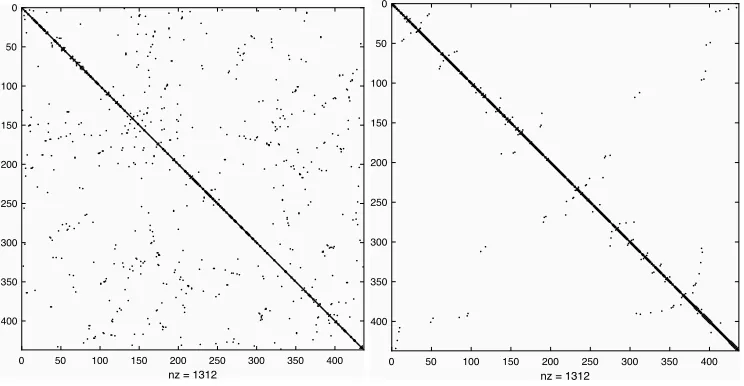
Figure 1Coefficient matrix structure before (left) and after (right) the ordering by the minimum degree permutation.
Parallelization of the code, still considering full non re-ordered matrices, allows for a reduction in the computational time from 458 s to 275 s, while the addition of matrix re-ordering substantially increases this reduction and the computational time drops to 55 s.
7
Conclusions
In this paper the extension of the global gradient algorithm, GGA, from the original steady state formulation to solve unsteady state problems via the admittance matrix method, NAMM, is explored. The reformulation of the admittance matrix method in the GGA framework allows interesting conclusions about the possible improvements in the NAMM efficiency. It is also reasonable to assume that any commercial steady-state software implementing an efficient algorithm for the GGA solution could be easily extended to obtain the unsteady-state solution provided by the NAMM formalization proposed in this paper. In this case, NAMM with an improved efficiency could be a formidable tool for inverse transient analysis and in calibration problems, where the reduced computational time is a fundamental requisite.
References
Amestoy, P. R., T. A. Davis, and I. S. Duff, 1996. An Approximate Minimum Degree Ordering Algorithm, SIAM Journal on Matrix Analysis and Applications, Vol. 17, No. 4, Oct., 886-905 Capponi, C., Ferrante, M., Zecchin, A.C., Gong, J., 2017. Leak Detection in a Branched System by
Inverse Transient Analysis with the Admittance Matrix Method, Water Resources Management 1– 15. doi:10.1007/s11269-017-1730-6
Capponi, C., Ferrante, M., 2018. Numerical investigation of pipe length determination in branched systems by transient tests. Water Science & Technology: Water Supply 18, 1062–1071. doi:10.2166/ws.2017.180
Chaudhry, M.H., 2014. Applied Hydraulic Transients, Third. ed. Springer New York, New York, NY. doi:10.1007/978-1-4614-8538-4
0 50 100 150 200 250 300 350 400
nz = 1312
0
50
100
150
200
250
300
350
400
0 50 100 150 200 250 300 350 400
nz = 1312
0
50
100
150
200
250
300
350
Ferrante, M., and Capponi, C., 2017. Calibration of viscoelastic parameters by means of transients in a branched water pipeline system. Urban Water Journal 1–7. doi:10.1080/1573062X.2017.1363254
George, A., and Liu, J. W-H. 1981. Computer Solution of Large Sparse Positive Definite Systems. Prentice-Hall, Englewood Cliffs, NJ.
Gilbert, J.R., Moler, C., Schreiber, R., 1992. Sparse Matrices in Matlab - Design and Implementation. Siam Journal on Matrix Analysis and Applications 13, 333–356.
Rossman, L.A., 2000. EPANET 2 Users Manual, U.S. Environmental Protection Agency, Washington, D.C., EPA/600/R-00/057.
Todini, E., Pilati, S., 1988. A Gradient Algorithm for the Analysis of Pipe Networks, in: B. Coulbeck and C.-H. Orr (Eds.), Computer Applications in Water Supply, J. Wiley and sons, 1–20.
Todini, E., Rossman, L.A., 2013. Unified Framework for Deriving Simultaneous Equation Algorithms for Water Distribution Networks. J Hydraul Eng-ASCE 139, 511–526. doi:10.1061/(ASCE)HY.1943-7900.0000703