https://doi.org/10.5194/gmd-10-3635-2017 © Author(s) 2017. This work is distributed under the Creative Commons Attribution 3.0 License.
PALM-USM v1.0: A new urban surface model integrated into the
PALM large-eddy simulation model
Jaroslav Resler1,2, Pavel Krˇc1,2, Michal Belda1,2,4, Pavel Juruš1,2, Nina Benešová1,3, Jan Lopata1,3, Ondˇrej Vlˇcek1,3, Daša Damašková1,3, Kryštof Eben1,2, Pˇremysl Derbek1, Björn Maronga5, and Farah Kanani-Sühring5
1Faculty of Transportation Sciences, Czech Technical University in Prague, Prague, Czech Republic 2Institute of Computer Science, The Czech Academy of Sciences, Prague, Czech Republic
3Air Quality Protection Division, Czech Hydrometeorological Institute, Prague, Czech Republic
4Department of Atmospheric Physics, Faculty of Mathematics and Physics, Charles University, Prague, Czech Republic 5Institute of Meteorology and Climatology, Leibniz Universität Hannover, Hannover, Germany
Correspondence to:Jaroslav Resler ([email protected]) Received: 9 March 2017 – Discussion started: 15 March 2017
Revised: 11 August 2017 – Accepted: 31 August 2017 – Published: 9 October 2017
Abstract. Urban areas are an important part of the climate system and many aspects of urban climate have direct ef-fects on human health and living conditions. This implies that reliable tools for local urban climate studies supporting sustainable urban planning are needed. However, a realistic implementation of urban canopy processes still poses a seri-ous challenge for weather and climate modelling for the cur-rent generation of numerical models. To address this demand, a new urban surface model (USM), describing the surface en-ergy processes for urban environments, was developed and integrated as a module into the PALM large-eddy simulation model. The development of the presented first version of the USM originated from modelling the urban heat island during summer heat wave episodes and thus implements primarily processes important in such conditions. The USM contains a multi-reflection radiation model for shortwave and long-wave radiation with an integrated model of absorption of ra-diation by resolved plant canopy (i.e. trees, shrubs). Further-more, it consists of an energy balance solver for horizontal and vertical impervious surfaces, and thermal diffusion in ground, wall, and roof materials, and it includes a simple model for the consideration of anthropogenic heat sources. The USM was parallelized using the standard Message Pass-ing Interface and performance testPass-ing demonstrates that the computational costs of the USM are reasonable on typical clusters for the tested configurations. The module was fully integrated into PALM and is available via its online repos-itory under the GNU General Public License (GPL). The
USM was tested on a summer heat-wave episode for a se-lected Prague crossroads. The general representation of the urban boundary layer and patterns of surface temperatures of various surface types (walls, pavement) are in good agree-ment with in situ observations made in Prague. Additional simulations were performed in order to assess the sensitivity of the results to uncertainties in the material parameters, the domain size, and the general effect of the USM itself. The first version of the USM is limited to the processes most rel-evant to the study of summer heat waves and serves as a basis for ongoing development which will address additional pro-cesses of the urban environment and lead to improvements to extend the utilization of the USM to other environments and conditions.
1 Introduction 1.1 Urban climate
One major phenomenon related to the urban climate is the urban heat island (UHI), i.e. the fact that an urban area may be significantly warmer than its surrounding rural areas, which mainly appears during evening and early night hours (Oke, 1982). The higher temperature is linked to the absorp-tion and retenabsorp-tion of energy by urban surfaces and to anthro-pogenic heat emissions, which can cause urban-to-rural tem-perature differences of several degrees Celsius. Moreover, buildings and other urban components can locally decrease the ventilation (e.g. Letzel et al., 2012), thus adding to ther-mal discomfort. Chemical processes, and consequently air quality, are also affected by the urban environment.
Effects of the urban heat island on living conditions have been the focus of urban planning for several decades in vari-ous cities, as it is anticipated that careful planning can allevi-ate some of these effects. However, developing adaptation and mitigation strategies requires state-of-the-art tools ap-plicable for urban climatology studies. The work presented in this paper started in the larger framework of the Ur-ban Adapt1 project, which focused on the development of such strategies for three major cities in the Czech Republic (Prague, Brno, and Pilsen). The aim was to provide as de-tailed a description of the street canyon conditions as pos-sible, going to the resolution of the order of a few metres. Below we provide a brief description of the methods typi-cally used for such a task and the motivation for developing a new urban surface model (USM).
Several possible approaches for studying urban climate have been used, ranging from observation analyses, over physical modelling, to numerical simulations (for a compre-hensive review, see e.g. Mirzaei and Haghighat, 2010; Moo-nen et al., 2012). In this context, a number of physical pro-cesses and their complex interactions must be taken into ac-count (e.g. Arnfield, 2003). Urban surfaces are affected by shortwave and longwave radiation, and energy is exchanged between the urban canopy and the atmosphere in various forms, including sensible and latent heat fluxes. These fluxes in turn, together with boundary layer processes and large-scale synoptic conditions, affect the turbulent flow of air. The complexity is further increased by the presence of vegetation and the pronounced heterogeneity of urban surface materials. For numerical modelling of urban climate processes, var-ious models and frameworks have been used (Mirzaei and Haghighat, 2010; Moonen et al., 2012; Mirzaei, 2015). One possible approach is to use a regional meteorological or cli-mate model. However, these models typically operate with horizontal resolutions of the order of hundreds of metres to tens of kilometres, and urban processes are treated using bulk parameterizations or single-/multi-layer urban canopy mod-els (e.g. Kusaka et al., 2001; Martilli et al., 2002). Thus, these models are much better suited to assessing the influence of urban environments on the larger-scale meteorology.
1http://urbanadapt.cz/en
A second approach is represented by standalone pa-rameterized models, e.g. the SOLWEIG model (Lindberg et al., 2008), RayMan (Matzarakis et al., 2010), the TUF-3D model (Krayenhoff and Voogt, 2007), the TUF-IOBES model (Yaghoobian and Kleissl, 2012, based on TUF-3D), TEB (Masson, 2000), or SUEWS (Järvi et al., 2011). These models treat some physical processes (e.g. radiation, latent heat flux, water balance), while they parameterize the air flow by means of statistical and climatological models or meteo-rological measurements.
The most complex approach is represented by a group of computational fluid dynamics (CFD) models. The ex-plicit simulation of the turbulent flow is computationally expensive; thus, different techniques have to be adapted to make calculations feasible, usually based on limiting the range of the resolved length scales and timescales of the turbulent flow. Most of the CFD models applied for ur-ban climatology studies today are models based on the Reynolds-averaged Navier–Stokes (RANS) equations, e.g. ENVI-met (ENVI-met, 2009), MITRAS (Schlünzen et al., 2003), MIMO (Ehrhard et al., 2000), and MUKLIMO_3 (Sievers, 2012, 2014). In RANS models, the entire turbu-lence spectrum is parameterized, and thus only the mean flow is predicted. This allows for use of relatively large time steps leading to moderate computational demands, but it im-plies physical limitations as interactions of turbulent eddies with the urban canopy cannot be explicitly treated. In or-der to overcome this deficiency, large-eddy simulation (LES) models can be employed. They use a scale separation ap-proach to resolve the bulk of the turbulence spectrum explic-itly, while parameterizing only the smallest eddies in a so-called subgrid-scale model. Examples of such models are e.g. PALM (Maronga et al., 2015), which can incorporate build-ings as explicit obstacles, the OpenFoam2 modelling sys-tem, which can use both LES and RANS solvers, or DALES (Heus et al., 2010).
However, many of the CFD models do not contain ap-propriate urban canopy energy balance models with an ex-plicit treatment of radiative fluxes. To overcome this defi-ciency, stand-alone energy balance models can be coupled to CFD models, recent examples being SOLENE-microclimat (Musy et al., 2015) or TUF-IOBES, which was coupled to PALM (Yaghoobian et al., 2014). These are usually one-way coupled systems in which the stand-alone model is used for the calculation of incoming/outgoing energy fluxes to/from any surface element, which are then imported into the CFD model. This means that CFD model dynamics are not con-sidered for the calculation of the energy fluxes, making this approach less precise than fully two-way integrated models.
Most of the CFD models are closed-source in-house solu-tions, complicating their scientific and technical validation. Furthermore, many of them are not designed to work on high-performance computing systems (HPC) with hundreds
to thousands of processor cores, limiting their range of ap-plications. Notable exceptions are the models PALM, Open-Foam, and DALES, which are available under a free license and can be run on HPC.
Regarding the task at hand, i.e. providing detailed infor-mation on the influence of urban surfaces and vegetation on pedestrian-level thermal comfort and air quality, LES mod-els can be considered to be the most appropriate and future-oriented since they can predict the turbulent air flow over a very complex surface with sufficient resolution. However, according to the authors’ research at the beginning of the study, there was no open-source LES model with an inte-grated energy balance solver for urban surfaces that would be able to account for the realistic implementation of vari-ous processes inside an urban canopy. Our attempts to in-tegrate some of the existing energy models (e.g. TUF-3D) into PALM led to serious technical difficulties due to the different scientific approaches of the particular models, in-compatible data structures, difficult parallelization, and other issues. The license compatibility was another issue. There-fore, we decided to start from scratch, extending existing LES model PALM with a new fully integrated USM module that explicitly describes energy exchanges in the urban envi-ronment. Due to the complexity of this task, the first version of PALM-USM was deliberately limited to the most impor-tant processes for modelling summer heat-wave episodes in fully urbanized areas. Further improvements and additions to this module are a current work in progress and will be real-ized within the next years (see also Sect. 6).
1.2 LES model PALM
PALM3is designed to simulate the turbulent flow in atmo-spheric and oceanic boundary layers. A highlight of PALM is its outstanding scalability on massively parallel computer architectures (Maronga et al., 2015). The model solves the non-hydrostatic incompressible Navier–Stokes equations in Boussinesq approximation. Subgrid-scale processes that can-not be resolved implicitly based on the numerical grid resolu-tion are parameterized according to the 1.5-order Deardorff closure scheme (Deardorff, 1980) with the modification of Moeng and Wyngaard (1988) and Saiki et al. (2000), assum-ing that the energy transport by subgrid-scale eddies is pro-portional to the local gradients of the mean quantities.
Prognostic equations are solved numerically, primarily using an upwind biased fifth-order differencing scheme (Wicker and Skamarock, 2002) and a third-order Runge– Kutta time-stepping scheme following Williamson (1980). Discretization in space is achieved using finite differences on a staggered Cartesian Arakawa-C grid (Arakawa and Lamb, 1977).
PALM includes several features, such as cloud micro-physics, a plant canopy model, and an embedded Lagrangian
3https://palm.muk.uni-hannover.de
particle model. In connection with the urban application, four other relevant schemes have already been implemented: a Cartesian topography scheme, representation of radiative exchange at the surface, large-scale forcing, and land-surface interactions with the atmosphere. The Cartesian topography scheme covers solid, impermeable, fixed flow obstacles (e.g. buildings) as well as terrain elevations (mountains, hills), with a constant-flux layer assumed between each surface ele-ment and the first grid level adjacent to the respective surface in order to account for friction effects. The representation of radiative exchange at the surface contains options to use either a simple clear-sky radiation parameterization or em-ploy the Rapid Radiation Transfer Model for Global Mod-els (RRTMG, e.g. Clough et al., 2005), which is coupled to PALM and is applied as a single-column model for each ver-tical column in the PALM domain. The large-scale forcing option enables forcing with data e.g. from mesoscale models via additional tendency terms, including an option for nudg-ing of the mean profiles. Finally, the implementation of land-surface interactions with the atmosphere is based on a sim-plified version of the Tiled European Centre for Medium-Range Weather Forecasts Scheme for Surface Exchanges over Land (TESSEL/HTESSEL, Balsamo et al., 2009) and its derivative implementation on the DALES model (Heus et al., 2010). PALM’s land-surface submodel (Maronga and Bosveld, 2017), hereafter referred to as PALM-LSM, further extends the surface parameterizations for impervious sur-faces on the ground (pavements, roads) by replacing upper soil layers with a pavement layer attributed with a specific heat capacity and heat conductivity.
However, none of the included schemes are suited for treating complex effects of the urban environment driven by the diverse physical properties of different urban surfaces (both horizontal and vertical), heat transfer within building walls, and heat fluxes between the urban surfaces and the at-mosphere. Also, the description of shortwave and longwave radiation budgets including shading and multi-reflection be-tween surfaces, as well as the absorption of radiation by plant canopies, have not been treated by PALM so far. Therefore, we developed the USM for PALM that is able to treat these processes using approaches described in the following sec-tion.
2 Urban surface model
a multi-reflection radiative transfer model (RTM) for the ur-ban canopy layer was developed, and coupled to the plant canopy model in order to calculate realistic surface radiative fluxes as input for the energy balance solver.
This first version of the USM was designed with the fo-cus on modelling summer heat-wave episodes in built-up ur-ban areas. The newly implemented methods hence concen-trated on the most relevant processes for such conditions. Limitations of the current version are e.g. no treatment of reflective surfaces and windows; only a basic building en-ergy model; simplification of some radiation-related pro-cesses (see Sect. 2.2.1 for details); a missing plant-canopy evapotranspiration model; and surfaces impervious to water. Possible impacts of these limitations are discussed in Sect. 4. Improvements of the USM and related PALM components are subject to ongoing development within the PALM com-munity.
2.1 Energy balance solver
The surface energy balance correlates radiative energy fluxes with sensible and latent heat fluxes between the surface skin layer and the atmosphere, as well as with the storage heat fluxes into soil and walls. In this first PALM-USM version, latent heat fluxes were omitted, since the purpose of this ver-sion was to simulate heat-wave episodes in fully urbanized areas. This limitation is discussed in Sect. 4.1. The energy budget is expressed in the form
C0 dT0
dt =Rn−H−G, (1)
where C0 andT0 are the heat capacity and temperature of the surface skin layer, respectively, t is the time,Rnis the net radiation, H is the turbulent sensible heat flux near the surface, and Gis the heat flux from the surface skin layer into the ground or material (i.e. pavement, walls, roofs). The list of all used symbols, their descriptions, and units can be found in the Supplement in Table S1.
The calculation of the heat transferHbetween the surface skin layer and the air is based on the equation
H=h(θ1−θ0), (2)
whereθ0 is the potential temperature at the surface andθ1 is the potential temperature of the air layer adjacent to the surface; and h is the so-called heat flux coefficient, which is parameterized for vertical surfaces according to Krayen-hoff and Voogt (2007), while for horizontal surfaces the pa-rameterization ofhfollows the default PALM-LSM formula-tion based on Monin–Obukhov similarity theory (Obukhov, 1971). The latter involves the calculation of a local friction velocity, for which stability effects are considered for hori-zontal surfaces, while stability for vertical surfaces is treated as neutral (i.e. law-of-the-wall scaling is used). The friction velocity is used to calculate both the surface momentum flux for each individual surface element and the coefficienthfor
A
B
C A
B
C D
θA
θB
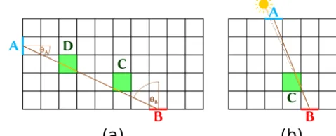
Figure 1. (a)View factor calculation (2-D simplification);(b)direct solar irradiation.
horizontal surface elements. The application of MOST for finite-sized surfaces is debatable as the theory is based on the assumption of horizontal homogeneity of the surface and flow, which is violated in urban areas. However, for lack of alternatives, it is the common modelling approach used in all state-of-the-art surface parameterization schemes (e.g. TUF-3D, Krayenhoff and Voogt, 2007; SUEWS, Järvi et al., 2011). The use of MOST in PALM as a boundary condition for buildings has been validated for neutral stratification by Letzel et al. (2008) and Kanda et al. (2013). Moreover, Park and Baik (2013) validated their LES results for non-neutral stratification against wind-tunnel data.
The heat transfer between surface skin layer and subsur-face layers follows the general formulation for the heat flux G:
G=3(T0−Tmatter,1), (3)
whereT0is the temperature of the surface skin layer,Tmatter,1 is the temperature of the outermost layer of the material, and 3is an empirical heat conductivity between the skin layer and the first grid level in the material.
The heat transfer within the material layers is calculated via the Fourier law of diffusion. This approach has been gen-eralized for different material types of the pavements, walls, and roofs, each structured into four layers; each layer of each material is described by its own properties (thickness, volumetric thermal capacity, and thermal conductivity). The diffusion equation is solved numerically describing the heat transfer from the surface into the inner layers. Boundary con-ditions of the deepest layer are prescribed in the configu-ration for particular types of surfaces and are kept constant throughout the simulation. The fluxG, calculated in the sur-face energy balance model, serves as a boundary condition for the outermost material layer.
2.2 Radiative transfer model 2.2.1 General concept
The USM receives radiation from the standard PALM so-lar radiation model at the top boundary of the urban canopy layer. Depending on the chosen radiation module in PALM, the separate direct and diffuse components of the downward shortwave radiation flux may or may not be available. In the latter case, a simple statistical splitting is applied based on Boland et al. (2008). The USM then adds a description of ra-diation processes in the urban canopy layer where multiple reflections are considered.
Radiation processes are modelled separately for shortwave (SW) and longwave (LW) radiation. Direct and diffuse SW solar radiation along with the relative position of the Sun, as well as the LW radiation from the atmosphere, is provided by PALM’s solar radiation model. Thermal emission from the ground, walls, and roofs is added as a source of long-wave radiation. For each time step, radiation is propagated through the 3-D geometry of the urban canopy layer for a fi-nite number of reflections, after which all of the radiation is considered fully absorbed by the surfaces. All reflections are treated as diffuse (Lambertian), and in each reflection, a portion of radiation is absorbed by the respective surface according to its properties (albedo and emissivity). The urban layer may contain an arbitrarily located plant canopy (trees and shrubs) described by a 3-D structure of leaf area density (LAD), which is treated as semi-opaque for the modelled SW radiation and transforms the absorbed radiation to heat (see Sect. 2.2.4).
Some radiation-related processes have been omitted in this first version, including absorption, emission, and scattering by air within the urban canopy layer, interaction of LW radi-ation with plant canopy, and thermal capacity of plant leaves (plant canopy is assumed to have the temperature of the sur-rounding air). The effects of these simplifications are dis-cussed in Sect. 4.
2.2.2 Calculation of view factors and canopy sink factors
For the calculation of irradiation of each face4 from dif-fuse solar radiation, thermal radiation, and reflected radia-tion, mutual visibility between faces of both real surfaces and virtual surfaces (top and lateral domain boundaries) has to be known. It is calculated using a ray tracing algorithm. Since this process is computationally expensive and hard to par-allelize (as rays can travel through the entire domain which is distributed on different processors), both the view factors (SVF) and the plant-canopy sink factors (CSF) are precom-puted during the model initialization. These factors can be 4A face is a unit of surface according to discretization by grid; it is a boundary between a grid box with terrain/building and an adjacent air-filled grid box.
saved to file and used for other simulations with the same surface geometry, or for the calculation of the mean radiant temperature (MRT) in the postprocessing.
For any two facesAandBwith mutual visibility, theview factorFA→B represents the fraction between that part of the radiant flux from faceAthat strikes faceBand the total radi-ant flux leaving faceA. For infinitesimally small areas ofA andB, adifferential view factorFAd→Bcan be written as FAd→B=dFA→B
dA(B) =
cosθAcosθB
π s2 , (4)
whereA(B)is the surface area of faceB,θAandθB are the angles between the respective face normals and the connect-ing ray, andsis the separation distance (ray length) (Howell et al., 2010); see Fig. 1a. Under the assumption thatsis much larger than the grid resolution, differential view factors are precomputed for all mutually visible face centres and used in place of view factors divided by target area. At the end, the differential view factors are normalized such that the sum of all normalized differential view factors with the same target face (B) multiplied by source area equals 1:
b
FAd→B= F d A→B
P
A0Fd
A0→BA(A0)
. (5)
If the view factors were known exactly, the sum
P
A0
FA0 →BA(A0)
A(B) would equal 1 (from the reciprocity rule
A(A)FA→B=A(B)FB→A). Therefore, the normalization guarantees that, in total, no radiation is lost or created by simplification due to discretization. Since the part of faceB’s irradiance that comes from faceAis computed as
Je,A→B=Ee,AA(A)FbAd→B, (6) whereEe,A is the radiosity of face A, we specifically pre-compute and store the value of
SVFA→B=A(A)FbAd→B (7)
which we call theirradiance factor. In case the ray tracing algorithm encounters an obstacle (i.e. wall or roof), the view-factor entry is not stored, indicating the absence of mutual visibility between the two respective faces.
The equations above describe radiative fluxes before ac-counting for plant canopy. For every ray that crosses a grid box containing plant canopy (i.e. a partially opaque box), a dimensionless ray canopy sink factor(RCSF) represents the radiative flux absorbed within the respective grid box normalized by the total radiative flux carried by the ray at its origin. For a rayA→B and a grid boxC, the RCSF is calculated as
RCSFC,A→B= 1− X
D
RCSFD,A→B !
1−e−αaCsC
, (8)
extinction coefficient. The sum in the first term represents cumulative absorption by all plant-canopy-containing grid boxesDthat have already been encountered on the ray’s path before reaching grid boxC(Fig. 1a).
After the entire ray is traced, the total transmittanceT of the rayA→Bpassing through plant canopy grid boxesC TA→B=1−
X
C
RCSFC,A→B (9)
is stored along with SVFA→B. Later in the modelling, when the radiant flux transmitted through SVFA→B is calculated, it is multiplied byTA→Bto account for the absorbed flux.
The actual radiant flux8ereceived by the grid boxCfrom the rayA→Bis equal to
8e,C,A→B=Ee,A·SVFA→B·A(B)·RCSFC,A→B. (10) The radiosity Ee,A of the source face is the only time-dependent variable in this equation. Therefore, the rest of this product can be precomputed during initialization, and summed up per source face in the form of acanopy sink fac-tor(CSF):
CSFC,A=
X
B
SVFA→B·A(B)·RCSFC,A→B. (11)
CSF represents the ratio between the radiant flux absorbed within plant canopy box Coriginating from faceAand the radiosity of faceA.
2.2.3 Calculation of per-face irradiation
At each time step, the total incoming and outgoing radiative fluxes of each face are computed iteratively, starting from the first pass of radiation from sources to immediate targets, followed by consecutive reflections.
In the first pass, the virtual surfaces (sky and domain boundaries) are used as sources of radiation by representing components of diffuse shortwave solar radiation and long-wave radiation from the sky. At this point, the real surfaces (wall facades, roofs, ground) are set to emit longwave radi-ation according to their surface temperature and emissivity. The precomputed view factors are then used to cast the short-wave and longshort-wave radiation from source to target faces.
Solar visibility has to be calculated for the quantification of the direct part of shortwave solar radiation. The solar an-gle is discretized for this purpose so that the solar ray always originates from the centre of the virtual face at the top of the urban layer or at lateral domain boundaries (see the real loca-tion of the Sun vs. the discretized localoca-tion (centre of faceA) in Fig. 1b). We have decided not to do the computationally expensive ray tracing after the precomputation phase is over; moreover, the total transmittance stored alongside the pre-computed view factor (see Eq. 9) is readily available. If there is no such view factor entry, it means that the discretized ray path is blocked by a wall or roof and the target face receives
no direct solar irradiation. For the purpose of calculating the actual amount of direct solar irradiation, an exact solar angle is used, not the discretized one.
After the aforementioned first pass of radiation from source to target surfaces has been computed, reflection is applied iteratively. At each iteration, a fraction of each sur-face’s irradiation from the previous iteration is reflected and the remainder is considered absorbed. The reflected fraction is determined by the surface’s albedo for shortwave radia-tion and by the surface’s emissivityεfor longwave radiation, where the longwave reflectivity results from(1−ε) accord-ing to Kirchhoff’s law. The reflected part is then again dis-tributed onto visible faces using the precomputed view fac-tors. After the last iteration, all residual irradiation is consid-ered absorbed. The number of iterations is configurable, and the amount of residual absorbed radiation can be displayed in the model output. In our experience, three to five iterations lead to negligible residue.
2.2.4 Absorption of radiation in the plant canopy The fraction of SW radiative flux absorbed by the plant canopy is calculated for the first pass as well as for all the suc-cessive reflection steps (these are described in Sect. 2.2.3).
For diffuse and reflected shortwave radiation, the amount of radiative flux absorbed by each grid box with plant canopy is determined using the precomputed CSF and radiosity of the source face (i.e. reflected radiosity for a real surface or diffuse solar irradiance for a virtual surface; see Eq. 10).
For the direct solar irradiance, the nearest precomputed ray path from the urban-layer bounding box (represented by vir-tual faceAin Fig. 1b) to the respective plant canopy grid box C is selected similarly to the direct surface irradiation de-scribed in Sect. 2.2.3. In case the grid boxCis fully shaded, no ray path is available. Otherwise, the transmittance of the path is known. The absorbed direct solar flux for the grid box Cis equal to
8e,C=Ee,dir·TA→C·
RR
b 1−e
−αaCsbdb
A0
C
, (12)
whereEe,diris the direct solar irradiance andA0Cis the cross-sectional area ofC viewed from the direction of the solar radiation. The fraction in Eq. (12) represents the absorbed proportion of radiative flux, averaged over each rayb that intersects the grid boxC, and is parallel to the direction of the solar radiation;sbis the length of the intersection. Since all grid boxes have the same dimensions, this fraction is pre-computed based on the solar direction vector at the beginning of each time step using discrete approximation.
2.3 Anthropogenic heat
The prescribed anthropogenic heat is assigned to the ap-propriate layer of the air, where it increases the potential-temperature tendencies at each time step. This process takes place after the surface energy balance is solved. The heat is calculated from daily total heat released into any particular grid box, and from the daily profile of the release specified for every layer to which anthropogenic heat is released. 2.4 USM module integration into PALM
The USM was fully integrated into PALM, following its modular concept, as an optional module, which directly uti-lizes the model values of wind flow, radiation, temperature, energy fluxes, and other required values. The USM returns the predicted surface heat fluxes back to the PALM core, where they are used in the corresponding prognostic equa-tions. It also adjusts the prognostic tendencies of air accord-ing to released anthropogenic heat.
Descriptions of real and virtual surfaces and their proper-ties are stored in 1-D arrays indexed to the 3-D model do-main. The crucial challenge of this part of the design is to ensure an efficient parallelization of the code, including an efficient handling and access of data stored in the memory during the simulation. The values are stored locally in par-ticular processes of the Message Passing Interface (MPI5), corresponding to the parallelization of the PALM core. Nec-essary access to values stored in other processes is enabled by means of MPI routines, including interfaces for one-sided MPI communication.
The configuration of the USM module is compatible with other PALM modules. Variables for instantaneous and time-averaged outputs of the USM are integrated into PALM’s standard 3-D NetCDF output files, and they are configured in the same way as the rest of the model output variables. The configuration options as well as the structure of in-put and outin-put files are described in the Supplement to this article. The Supplement also contains the list and descrip-tion of needed surface and material parameters of urban sur-faces, plant-canopy data, and anthropogenic-heat data. The model PALM with its USM module is hereafter referred to as PALM-USM, which is freely available under the GNU Gen-eral Public License (see the Code availability section).
3 Evaluation and sensitivity tests of the USM
In order to evaluate how well the USM represents urban sur-faces’ temperatures (of e.g. walls, roofs, and streets), a sum-mer heat-wave observation campaign in an urban quarter of Prague, Czech Republic, was carried out (see Sect. 3.1). By means of PALM-USM, urban-quarter characteristics and the campaign’s meteorological conditions were simulated (see
5http://mpi-forum.org
Sect. 3.2) and model results evaluated against the observa-tions (see Sect. 3.3).
3.1 Observation campaign
The campaign was carried out at the crossroads of Dˇel-nická street and Komunard˚u street in Prague, Czech Repub-lic (50.10324◦N, 14.44997◦E; terrain elevation 180 m a.s.l.). This location was selected in coordination with the Prague Institute of Planning and Development as a case study area for urban heat island adaptation and mitigation strategies. This particular area represents a typical residential area in a topographically flat part of the city of Prague with a combi-nation of old and new buildings and a variety of other urban components (such as yards or parking spaces). The streets are oriented in the north–south (Komunard˚u) and west–east (Dˇelnická) directions, roughly 20 and 16 m wide, respec-tively. The building heights alongside the streets range ap-proximately from 10 to 25 m. The area does not contain much green vegetation and the majority of the trees is located in the yards. The neighbourhood in the extent of approximately 1 km2 has similar characteristics to the study area (see the aerial photo in Fig. 2).
Measurements were conducted from 2 July 2015, 14:00 UTC to 3 July 2015, 17:00 UTC. The timing of the measurement campaign was chosen to cover a typical sum-mer heat-wave episode.
3.1.1 Measurements
Wall and ground surface temperatures were measured by an infrared camera – FLIR SC660 (FLIR, 2008). The thermal sensor of the camera has a field of view of 24 by 18◦ and a spatial resolution (given as an instantaneous field of view) of 0.65 mrad. The spectral range of the camera is 7.5 to 13 µm, and the declared thermal sensitivity at 30◦C is 45 mK. The measurement accuracy for an object with a temperature between+5 and+120◦C, and given an ambient air temper-ature between +9 and +35◦C, is ±1◦C, or ±1 % of the reading. The camera offers a built-in emissivity-correction option, which was not used for this study. Apart from the in-frared pictures, the camera allows us to take pictures in the visible spectrum simultaneously.
Figure 2.Aerial photo of the studied area.
Figure 3.Observation locations. Arrows depict the orientation of the camera view. Url of the map: https://mapy.cz/s/12Qd8.
simultaneously, starting at observation location 1 every full hour and continuing through observation locations 2, 3, etc. This provided a series of 28 temperature snapshots per loca-tion with an approximately 1 h time step. The exact record-ing time of each picture was used for further processrecord-ing and evaluation of the model.
The pictures were further postprocessed. First, the infrared pictures were converted into a common temperature scale
+10 to +60◦C. Second, the pictures were transformed to
overlap each other in order to correct for slight changes in camera position between the measurements, as the camera was carried from one location to another. Third, several eval-uation points were selected for each view to cover various surface types in order to evaluate the model performance un-der different surface parameter settings (different surface ma-terials and colours) and under different situations (fully ir-radiated or shaded areas). That is, selected surface materials comprised old and new plastered brick house walls as well as modern insulated facades for vertical surfaces, and pavement or asphalt for the ground observation location. With regard to colours, the evaluation points were placed on both dark and light surfaces, with special interest in places where light and dark materials are located side-by-side, thus allowing one to inspect different albedo settings under roughly the same ir-radiance conditions. Some points were placed on wall areas, which are temporarily (in the diurnal cycle) shaded by trees or buildings, in order to test how the shading works in the model.
Apart from infrared camera scanning, the air temperature was measured once an hour at observation location 1 at the edge of the pavement, about 2 m apart from the wall and 2 m above ground, and not in direct sunlight. A digital thermome-ter with an exthermome-ternal NTC-type thermistor measuring probe (resolution of 0.1 K and declared accuracy of 1 K) was used. This on-site measurement did not meet requirements for the standard meteorological measurement; therefore, we refer to it as the indicative measurement later in the text.
Figure 4.Meteorological conditions from station Prague, Karlov, and spatially averaged traffic heat flux from 1 to 4 July. The shaded area marks the time of the observation campaign.
Prague, Klementinum; Prague, Karlov; Prague, Kbely; and Prague, Libuš. Station Prague, Klementinum (50.08636◦N, 14.41634◦E; terrain elevation 190 m a.s.l., 3 km away from the crossroads of interest) was used as supplementation to the on-site indicative measurement. The temperature at this station is measured on the north-facing wall, 10 m above the courtyard of the historical building complex, and it can be used as another reference for the air temperature in-side the urban canopy. Station Prague, Karlov (50.06916◦N, 14.42778◦E, 232 m a.s.l.; 4.3 km away), can be considered representative for the city core of Prague as it is located in the centre of the city. Station Prague, Kbely (50.12333◦N, 14.53806◦E, 285 m a.s.l.; 6.7 km away), is located at the bor-der of the city and serves as a reference for regional back-ground suburban meteorological conditions. Station Prague, Libuš (50.00778◦N, 14.44694◦E, 302 m a.s.l.; 10 km away), is located in the city suburb and it is the only station with sounding measurements in the area. Radiosondes are re-leased three times a day (00:00, 06:00, 12:00 UTC).
3.1.2 Weather conditions
The weather during the campaign was influenced by a high-pressure system centred above the Baltic Sea. The mete-orological conditions at Prague, Karlov station, are shown in Fig. 4. Winds above rooftop were weak, mostly below 2.5 m s−1, and often as low as 1 m s−1 from easterly direc-tions. The maximum measured wind speeds of 3–4 m s−1 were observed in the afternoons at the beginning and at the end of the campaign. According to the atmospheric sounding,
a low-level jet from the south and south-east was observed during the night, with a maximum wind speed of 10 m s−1 at 640 m a.s.l. (950 hPa) (not shown). The temperature ex-ceeded 30◦C in the afternoons and dropped to 20◦C at night. The sky was mostly clear with some clouds during the day-time on 1 July and high-altitude cirrus forming in the morn-ing and afternoon on 3 July. The highest values of relative humidity occurred at night (65 %), dropping to 30 % during the day. The time of the sunset was 19:15 UTC on 2 July 2015, and the time of sunrise and solar noon on 3 July was 02:58 and 11:06 UTC.
3.2 Model set-up and input data for USM
To assess the validity of the model formulation and its per-formance in real conditions, the model was set up to simulate the measured summer episode described in Sect. 3.1. The to-tal simulation time span was 48 h, starting on 2 July 2015, 00:00 UTC.
3.2.1 Model domain
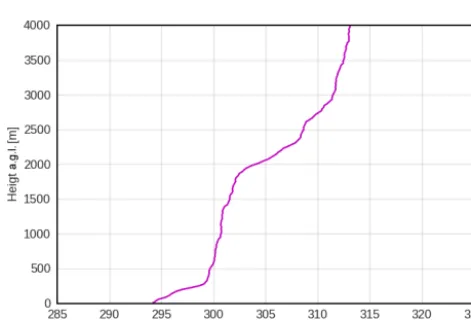
com-Figure 5.Initial vertical profile of potential temperature (θ) as used for initialization of PALM.
putational demands feasible. This poses some limitation to the turbulence development during the daytime, where the largest eddies usually scale with the height of the boundary layer. These eddies could not be captured well with this con-figuration. The effects of the limited horizontal size of the domain on model results will be discussed in Sect. 4. 3.2.2 Boundary and initial conditions
Lateral domain boundaries were cyclic, which can be envi-sioned as an infinite repetition of the simulated urban quar-ter. This is a reasonable approximation, since the surrounding area has similar characteristics to the model domain; thus, the character of the flow can be considered similar. The bot-tom boundary was driven by the heat fluxes as calculated by the energy balance solver (see Sect. 2.1). At the top of the domain, Neumann boundary conditions were applied for po-tential temperature and relative humidity, while a Dirichlet boundary was set for the horizontal wind. A weak Rayleigh damping with a factor of 0.001 was applied to levels above 3000 m. The indoor temperature was fixed at 22◦C during the entire simulation.
The initial vertical profile of potential temperature of air was derived from the sounding measurement in the out-skirts of Prague, Libuš station, from 2 July 2015, 00:00 UTC (see Fig. 5). At midnight, a stable layer had developed near the surface, extending to a height of about 300 m. Above, a residual layer with slightly stable stratification ranged up to the inversion at around 1900 m. The capping inversion had a strength of about 5 K, with the stable free atmosphere aloft. The temperature of walls, grounds, and roofs was initialized from a 24 h spin-up simulation.
3.2.3 Large-scale forcing
To account for the processes occurring on larger scales than the modelling domain but still affecting the processes in-side the domain, the large-scale forcing option of PALM was used. The effect of large-scale conditions is included via geostrophic wind and large-scale advection tendencies for temperature and humidity. The forcing quantities can de-pend on both height and time while being horizontally ho-mogeneous. Nudging of PALM quantities towards the large-scale conditions was enabled for the free atmosphere lay-ers with a relaxation time of 7 h. Inside the boundary layer nudging was disabled. Large-scale forcing and nudging data were generated based on a run with the WRF meso-scale numerical weather prediction model (version 3.8.1, Ska-marock et al., 2008). The WRF simulation domain cov-ered a large part of Europe (−1.7–34.7◦ longitude, 41.4– 56.7◦ latitude; 9 km horizontal resolution, 49 vertical lev-els). Standard physics parameterizations were used, includ-ing the RRTMG radiation scheme, the Yonsei University PBL scheme (Hong et al., 2006), a Monin–Obukhov simi-larity surface layer, and the Noah land surface model (Tewari et al., 2004). The urban parameterization was not enabled, in order to avoid double counting of the urban canopy effect which is treated by PALM-USM. The configuration of the WRF model corresponds to the prediction system routinely operated by the Institute of Computer Science of the Czech Academy of Sciences.6
The output of the WRF model was compared to measure-ments from the four Prague stations (see Sect. 3.1.1). The overall agreement between the simulated values and the ob-servations is reasonable and corresponds to long-term evalu-ations done earlier. For the period of 1–5 July (see Fig. S1), WRF shows a cold bias. The largest bias occurs in the ur-ban Prague, Klementinum station (city centre), which is as expected given the urban parameterization not being enabled in the WRF model. On the other hand, the comparison with Prague, Kbely station (closest background station to the area of interest), shows only a small bias (see also the time series in Fig. S2). Also, the comparison with vertical profiles of temperature from Prague, Libuš station, shows good agree-ment (see Fig. S3). Despite the slight cold bias of the WRF simulation, we take the WRF-derived values as the best in-puts available.
3.2.4 Surface and material parameters
Solving the USM energy balance equations requires a num-ber of surface (albedo, emissivity, roughness length, ther-mal conductivity, and capacity of the skin layer) and volume (thermal capacity and volumetric thermal conductivity) ma-terial input parameters. When going to such a high resolu-tion as in our test case (∼2 m), the urban surfaces and wall materials become very heterogeneous. Any bulk parameter
setting would therefore be inadequate. Instead, we opted for a detailed setting of these parameters wherever possible. To obtain these data, a supplemental on-site data collection cam-paign was carried out and a detailed database of geospatial data was created. This includes information on wall, ground, and roof materials and colours which was used to estimate surface and material properties. Each surface is described by material category and albedo. Categories are assigned to parameters estimated based on surface and storage material composition and thickness. The parameters of all subsurface layers of the respective material were set to the same value. The parametersC0and3(see Eqs. 1 and 2) of the skin layer are inferred from the properties of the material near the sur-face, which may differ from the rest of the volume. Parame-ters associated with particular categories are given in Supple-ment Table S2. A tree is described by its position, diameter, and vertically stratified leaf area density. Building heights were available from the Prague 3-D model, maintained by the Prague Institute of Planning and Development.7All de-scriptions of surfaces and materials and their properties were collected in GIS formats and then preprocessed into the USM input files corresponding to the particular domain set-up.
3.2.5 Anthropogenic heat
Anthropogenic heat sources for our particular case are dom-inated by heat from fuel combustion in cars (see also the dis-cussion in Sect. 4). Based on Sailor and Lu (2004), we as-sume the average heat release to be 3975 J per vehicle per metre of travel. Traffic intensities and hourly traffic factors are based on the annual traffic census data. The traffic in-tensities vary for different arms of the crossroads and traffic directions. The total count of vehicles passing through the crossroads is 12 000 vehicles per day, and the intensity of the busiest road (western arm of the west–east street) is 6000 vehicles per day. The heat produced by the cars along their trajectories is released into the first model layer and spatially distributed into the model grid cells that correspond to the traffic lanes. Temporal distribution is done using prescribed hourly factors. The time factors are the same for all traffic lanes. Values of anthropogenic heat are 42 W m−2 on aver-age (spatially and temporally), while the maximum value is 142 W m−2(busiest road arm, peak hour). Those values refer to heat fluxes directly above the traffic lanes. The mean daily traffic heat flux averaged over the entire domain is 2 W m−2. The daily course of the traffic heat release is plotted in Fig. 4. It has been shown before that for this particular case (with strong solar irradiance, high temperatures, and only moderate traffic) the inclusion of anthropogenic heat from transporta-tion does not result in a noticeable change in temperatures and heat fluxes (Juruš et al., 2016).
7http://www.geoportalpraha.cz
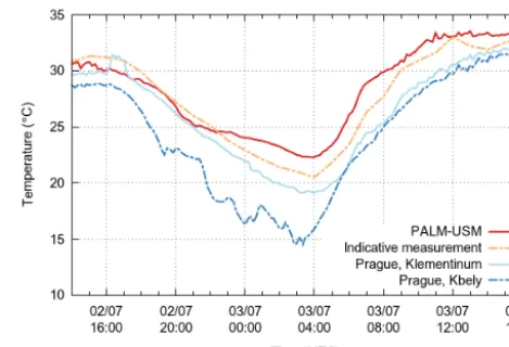
Figure 6.Air temperatures obtained from PALM-USM for loca-tion 1 in comparison to measured temperatures.
3.3 Evaluation of PALM-USM
First we compare the air temperatures from PALM-USM to the measurements taken during the observation campaign. Figure 6 shows the air temperature course calculated by the PALM-USM at observation location 1 at 2 m above ground. This temperature is compared to the indicative measurement taken at the same place and also to automatic weather stations Prague, Klementinum, and Prague, Kbely. The indicative measurement together with station Prague, Klementinum, represent the conditions inside the urban canopy, and as such, the results of PALM-USM should correspond to those values. Prague, Kbely station is plotted as a representative of the out-skirts of the city. The UHI effect is clearly visible, especially at night, when the temperature outside of Prague drops down to 15◦C, while on the street level, it drops to 20◦C only. This effect is less pronounced during the day, when the tem-perature difference is only 2–3◦C. This reflects the known fact that the UHI is basically a nighttime effect (Oke, 1982). The street-level air temperature as simulated by PALM-USM is in agreement with both measurements during the daytime of 2 July, but starting from 21:00 UTC, the decrease in the modelled temperature weakens, gradually leading to overes-timations of up to 2◦C in the morning of 3 July.
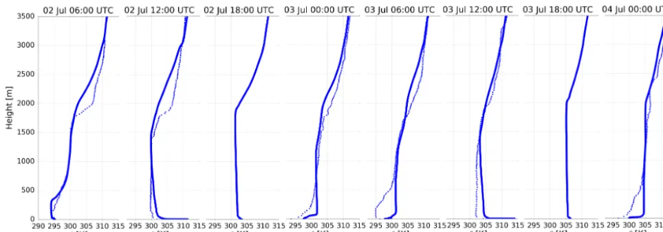
The vertical structure of the potential temperature from PALM-USM is shown together with radiosonde observations from station Prague, Libuš, in Fig. 7. As this is a suburban background station (10 km away), the profiles are not truly comparable, especially near the surface, where effects of the UHI are expected in the PALM-USM data. The Libuš profiles are considered here mainly as a representation of the general meteorological situation in the area of interest.
Figure 7.The vertical profiles of potential temperature modelled by PALM (solid line) and supplemented by radiosonde observations from station Prague, Libuš (except for hour 18; dotted line). Displayed are profiles from 2 July, 06:00 UTC to 4 July, 00:00 UTC with a 6 h time step.
particularly on 2 July (12:00 UTC). This can be attributed to the higher amount of heat released by the surfaces of densely built-up urban areas, as compared to the surfaces of subur-ban regions where the radiosonde was released. Moreover, it is visible that the potential temperature profile produced by PALM-USM displays an unstable stratification through-out the CBL on both days, while the observations show the expected nearly neutral profile. We will later see that this is an effect of the limited horizontal model domain that inhibits the free development of the largest eddies and thus is limit-ing the vertical turbulent mixlimit-ing of warm air from the surface and relatively cold air from above. The result is an unstable layer with somewhat overly high near-surface temperatures.
During nighttime, a stable boundary layer developed in both LES and observations (due to nocturnal radiative cool-ing). As expected, this cooling is more rigorous in the (sub-urban) measurements, so that the stable layer was able to extend to heights of 500 m, whereas PALM-USM predicts a stable layer of not more than 100 m vertical extent (see 00:00 UTC on 3 and 4 July). This result is in agreement with what was already shown in Fig. 6 and is a known feature of the UHI (Oke, 1982).
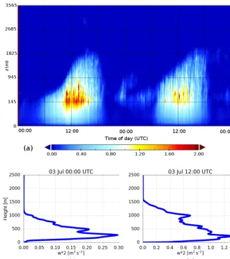
Figure 8a–c shows the temporal development of the turbu-lence, which is here represented by the variance of vertical velocity. The diurnal turbulence cycle is very clearly visible, with maximum intensities of 1.4 m2s−2around noon located in the well-mixed part of the boundary layer (Fig. 8c). Ide-ally, it would show a clear maximum in the middle of the boundary layer, but two processes avoid this. First, the ur-ban canopy arranges the release of heat at different heights above the ground surface, and second, the limited horizon-tal model domain does not allow for a free development of turbulence. Figure 8a further shows that the turbulence im-mediately starts to decay after sunset, which is accompanied by the development of a stable boundary layer near the
sur-face (not shown here). During nighttime, the turbulence fur-ther decays and the maximum values of the variance reduce to 0.3 m2s−2. Due to the continuously heating urban surface layer, however, turbulence is kept alive until the next morn-ing (see also Fig. 8a).
Next, in order to assess how well the model is able to model the energy transfer between material and atmosphere, we compare modelled values to on-site measurements of sur-face temperatures captured by the infrared camera. Here we present results from five selected locations, chosen to cover wall orientations to all cardinal directions and the ground: lo-cation 3 (south-facing wall) in Fig. 9, lolo-cation 4 (west-facing wall) in Fig. 10, location 7 (north-facing wall) in Fig. 11, lo-cation 9 (east-facing wall) in Fig. 12, and lolo-cation 8 (ground) in Fig. 13. Corresponding surface and material parameters for all evaluation points can be found in Tables S2 and S3 in the Supplement. Results for all nine locations are also dis-played in the Supplement (Figs. S4–S12). In general, PALM-USM captures the observed daily temperature patterns very well. The temperature values during the daytime are cap-tured reasonably well, while the model slightly overestimates nighttime temperatures.
Figure 8. (a)Time–height cross section of the variance of the vertical velocity component (top), and vertical profiles of the same quantity at two selected times:(b)3 July 00:00 UTC and(c)3 July 12:00 UTC (bottom).
for points 2, 3, and 4, too. The observation that the model overestimates values at some evaluation points located in the lowest parts of the buildings can also be made at other obser-vation locations (see location 4, Fig. 10, point 1, or location 5, Fig. S8, point 1).
In Fig. 9, daytime temperatures of points 1 and 2 are cap-tured quite well, while the model overestimates the temper-ature in point 3. In reality, this point is shaded by an alcove until 08:10 UTC (see the IR picture in Fig. S13) and thus it is irradiated approximately 1 h later than point 1. As a con-sequence, the increase in its temperature is delayed and the reached maximum temperature is 4◦C lower than in point 1. This facade unevenness is not resolved by the topography model in PALM and it thus predicts the same values for points 1 and 3.
Figure 10 shows the same comparison for a west-facing wall in the southern arm of the north–south street mea-sured from location 4. The temperature course in point 7 demonstrates the effect of surface shading by a tree that
ob-structs the solar radiation at this location between 13:10 and 14:50 UTC. This leads to a decrease in surface temperature between 13:00 and 15:00 UTC, whereas the surface temper-ature at the other points keeps increasing. This shading ef-fect can also be seen in Fig. 12 for point 5, which is shaded by a tree between 06:15 and 08:15 UTC. Both cases are cor-rectly represented by the model. Another illustration of tree shading is in Fig. S14.
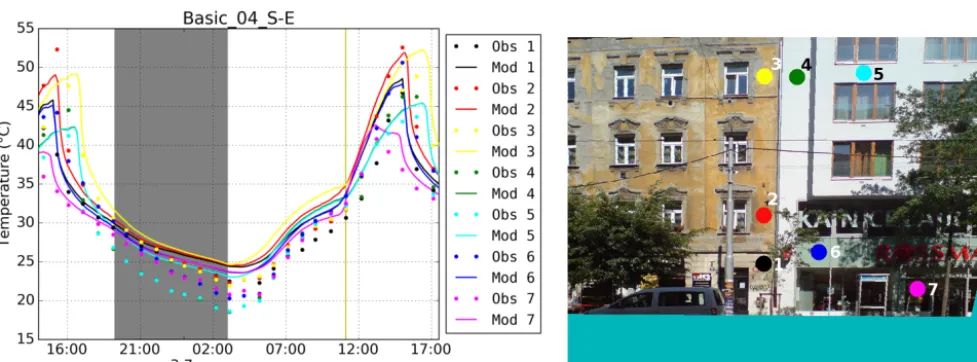
Figure 9.Comparison of modelled and observed surface temperatures from observation location 3 (50.10354◦N, 14.45006◦E) – view of the south-facing wall. The graph shows comparisons for selected evaluation points for the period of the observation campaign from 2 July 2015, 14:00 UTC to 3 July 2015, 17:00 UTC. The solid line represents modelled values, while the dots show the observed values. The shaded area depicts nighttime and the yellow vertical line depicts solar noon.
Figure 10.As for Fig. 9 for location 4 (50.10288◦N, 14.44985◦E) – view of the west-facing wall.
15:00 UTC). The possible reason for this overestimation is discussed later in Sect. 4.
Figure 12 shows the east-facing wall of the northern arm of the north–south street. We can observe the effect of shading by opposite buildings here. As the Sun rises and the shade cast by opposite buildings moves downward in the morning, the Sun gradually irradiates points 3 (from 04:45 UTC), 2 (from 05:40 UTC), and 1 (from 06:10 UTC). This is reflected in observations and also in model results, although the mod-elled temperature in point 3 starts to increase somewhat later than the observed temperature at the same point due to the discretized geometry of the buildings on the opposite side of the street. The effect of the shading of east-facing walls dur-ing the sunrise is further visible in Fig. 15.
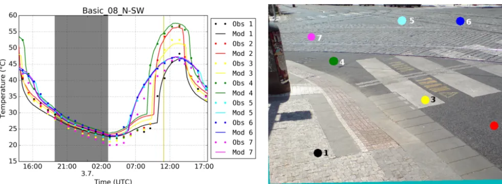
Finally, Fig. 13 shows the measurement of the ground sur-face temperature. The model captures the maximum values well, which are higher for asphalt (points 2, 3, and 4) than for paving blocks (points 1, 5, 6, and 7). The lower tem-perature of the white crosswalk, represented in the model as a one-grid-width belt with higher albedo, is reflected in the model results as well. Also, the time when the temperature starts to increase in the morning is captured with some minor discrepancies, owing to the discretized representation of the surrounding buildings.
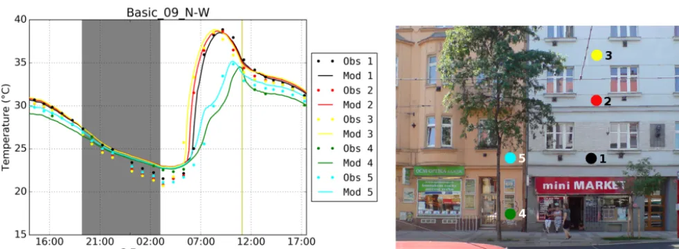
Figure 11.As for Fig. 9 for location 7 (50.10329◦N, 14.45040◦E) – view of the north-facing wall.
Figure 12.As for Fig. 9 for location 9 (50.10354◦N, 14.45006◦E) – view of the east-facing wall.
surfaces (e.g. all south-facing walls), the different wall prop-erties lead to differently warmed surfaces. Further, cool spots resulting from shading by trees are clearly visible. This view also demonstrates the effect of transforming the real urban geometry into the regular modelling grid. The detailed view of east-facing walls in the north–south street in the morning of 3 July is shown in Fig. 15. This picture shows surface tem-peratures after the sunrise at 06:00 and 08:00 UTC. The view displays the effects of shading by buildings on the opposite side of the street as well as the thermal inertia of the material and the impact of different material properties.
3.4 Sensitivity tests
3.4.1 Sensitivity to the dynamics of surface heat fluxes
simula-Figure 13.As for Fig. 9 for location 8 (50.10340◦N, 14.45007◦E) – view of the ground on the crossroads.
Figure 14.Modelled surface temperatures for the entire domain on 3 July at 12:00 UTC. Green areas represent vegetation (trees).
tion ran for 5 h to reach a quasi-steady state. Figure 16 shows the horizontal cross section of the time-averaged (1 h) ver-tical velocity at 10 m a.g.l.Figures correspond to simulation time 3 July at 14:00 UTC, when west- and south-facing walls were fully irradiated and heated up by the Sun. The wind above the roof top was north-west and its strength was about 2 m s−1. In the PALM-noUSM case, a typical vortex per-pendicular to the street axis in the west–east oriented street and in the southern part of the south–north oriented street was formed. In the reference case, however, the non-uniform heat flux was heating the air on the south- and west-facing walls, changing the strength of the street vortex. This effect is more intensely pronounced in the southern arm of the north– south oriented street where the strong vortex observed in case PALM-noUSM has significantly weakened. In Fig. 17 it be-comes evident that the entire flow circulation pattern within
this street arm had changed, leading to a change in the vortex orientation.
The accurate prediction of the canyon flow is an essen-tial prerequisite, among others, for the accurate prediction of pollutant concentrations at street level and their vertical mix-ing. Our results – in line with previous studies – show that an interactive surface scheme is a crucial part of the urban modelling system and alters the canyon flow significantly. 3.4.2 Sensitivity to material parameters
Figure 15.Modelled surface temperatures of the east-facing walls in the north–south street after the sunrise on 3 July at 06:00 UTC (top) and 08:00 (bottom) UTC.
Figure 16.Horizontal view of modelled vertical velocity (1 h average) at 10 m a.g.l.on 3 July, 14:00 UTC.(a)presents a stationary simulation without USM with constant surface heat fluxes and(b)the reference simulation with USM enabled.
The uncertainty of the input parameters is high, though. In order to estimate related uncertainties of model results, a se-ries of simulations was performed where one parameter was changed per simulation. The tests included the increase and decrease in albedo, the thermal conductivity of both the ma-terial and the skin layer, and the roughness length of the sur-face. The albedo was modified by±0.2 and all other param-eters were adjusted by±30 % of their respective value. The sensitivities of the surface temperature at selected locations and evaluation points are presented in Fig. 18. The largest changes in model output are generally observed during day-time. The model behaves according to the physical meaning of the parameters: decreased roughness lowers turbulent ex-change of heat between the surface and air, leading to the increase in surface temperature when the air is colder, which is usually the case in our simulation. A decrease in rough-ness to 70 % leads to the increase in temperature by up to 4◦C. A decrease in thermal conductivity leads to more in-tense heating of the surface when the net heat flux is positive
(usually during daytime) and to less intense cooling when it is negative (usually during night). The decrease in the albedo leads to higher absorption of SW radiation and an increase in the surface temperature during daytime. The sensitivity of the modelled surface temperature can reach up to 5◦C.
Figure 17.Wind field. Simulation without USM with prescribed surface heat fluxes(a)and with USM(b). View from the southern border of the domain towards the crossroads.
Figure 18. The sensitivity of PALM-USM to changes in surface and material parameters:(a)for the west-facing wall measured from location 1 for evaluation point 1, (b) for the ground measured from location 8 for evaluation point 3, and(c)for the east-facing wall measured from location 9 for evaluation point 5. ref is the reference run; other lines correspond to the increase (dashed line) and decrease (solid line) in the respective parameters with respect to the reference run: albedo was increased/decreased by 0.2, thermal conductivity of materials and skin surface layer (conductivity) was increased/decreased by 30 %, and so was the roughness length (roughness). Obs is the measurement in the evaluation point.
some limitation of the set-up, or the model itself. Some pos-sible reasons are discussed in Sect. 4.
4 Discussion
The deficiencies in the model’s description of reality and the discrepancies against observations may arise from limita-tions, simplificalimita-tions, and omissions within the model itself and from limited exactness, representativity, and appropriate-ness of the model set-up.
4.1 Limitations of the model
The USM and its radiative transfer model (RTM) assume only a diffuse reflection and do not treat windows. In our configuration, specular reflection can play a role for glossy surfaces like flagstones and glass. Windows also transmit
to 70 W m−2during the day, and since the opposite walls rep-resent about one-third to half of the visible area, these differ-ences are not negligible and may be responsible at least partly for the overestimation of the surface temperature of north-facing walls. This suggests that an extension of the USM by a proper window model is very desirable.
The RTM also simulates only a finite, configured number of reflections. After that, the remainder of reflected irradiance is considered fully absorbed by the respective surface. The amount of absorbed residual irradiance is available among model outputs and it can be used to find an optimum number of reflections until the residual irradiance is negligible. The optimum setting depends on the albedo and emissivity of the surfaces. In our set-up, the residual irradiance was below 1 % of the surface’s total at most surfaces after three reflections, and it was negligible after five reflections.
The current version of the RTM model does not simu-late absorption, emission, and scattering of radiation in the air within the urban canopy layer; thus, it is not suitable for modelling of situations with extremely low visibility like fog, dense rain, or heavy air pollution. However, under clear air conditions and in an urban set-up where typical distances of radiatively interacting surfaces are of the order of metres or tens of metres, these processes are negligible8. Most of the solar radiation’s interaction with the atmosphere happens on the long paths from top of atmosphere to ground and during the interaction with clouds, i.e. above the urban layer, where the method of modelling of these processes depends on the selected solar radiation model in PALM.
The USM is currently coupled to PALM’s simple clear-sky radiation model, which provides only limited information on sky longwave radiation, and it does not provide air heating and cooling rates. This limitation will be overcome in the near future when the USM will be coupled to the more ad-vanced RRTMG model in PALM.
Shading by plant canopy is only modelled for shortwave radiation; in the longwave spectrum, the plant canopy is con-sidered fully transparent. Typical daily maxima of SW ra-diative fluxes (mostly from direct solar radiation) are much higher than maxima of LW fluxes. Moreover, much of the LW heat exchange is compensated when surfaces are near ra-diative equilibrium. Therefore, for the LW shading by plant canopy to cause significant changes in the heat fluxes, two conditions must occur simultaneously: the plant canopy and the affected surface have to occupy a large portion of each other’s field of view (e.g. a large and dense tree close to a wall); and the temperature of the plant canopy, the affected surface, and the background field of view have to differ sig-nificantly (e.g. the wall is under direct sunlight and the plant canopy is shaded or cooled by convection).
8Using MODTRAN (Berk et al., 2014) for a clean-air sum-mer urban atmosphere, transmissivity for 10 µm radiation (i.e. peak wavelength of black-body radiance at 300 K) per 1 km of air is ap-proximately 0.85, which equals 0.998 per 10 m.
To illustrate the amount of affected heat flux, let us pro-pose a simple realistic scenario where these effects are very strong. Let us have two opposing walls, each occupying 50 % of the other’s field of view (without regard for plant canopy), and let us add a row of trees directly between the walls, blocking 30 % of the mutual radiative exchange between the walls. Let the temperature of the ambient air, one of the walls, and the plant canopy be 300 K, and let the other wall heat to 320 K due to strong direct sunlight.
Under these conditions, the cool wall would be receiving 68 W m−2 of excess total radiative flux (absorption minus emission) due to the opposing wall being hotter. The hot wall would be losing the same excess total flux due to the oppos-ing wall beoppos-ing cooler, both when not accountoppos-ing for shadoppos-ing by plant canopy. With the plant canopy, the cool wall would only be receiving 41 W m−2of excess total flux from the op-posing wall and the remaining flux of 21 W m−2would be absorbed by the plant canopy. The hotter wall would experi-ence the same radiative cooling as without plant canopy.
With regard to our test scenario, we accepted the simpli-fication, considering that the demonstrated omission would affect only a few spots in the modelled domain. Modelling of LW interaction with plant canopy is planned for the next version of the model.
Plant leaves are treated in the USM as having zero ther-mal capacity and a similar temperature to the surrounding air. Any radiation absorbed by leaves directly heats the sur-rounding modelled air mass. In reality, plant leaves are thin, they have a large surface area, and they readily exchange heat with air. This simplification is common among radia-tive transfer models (see e.g. Dai et al., 2003) and it is also in accordance with the current implementation of the non-urban plant canopy model in PALM.
Figure 19.As for Fig. 7 for the idealized simulation with an enlarged domain (see Sect. 4).
N
Figure 20. Comparison of the duration of the model run and the time spent in the chosen subprocesses of the model(a)and detailed comparison of parts of the USM model(b). Meaning of data series: “no USM” the run of PALM with USM switched off, “USM no canopy” the run with USM with no plant canopy, “USM canopy” run with USM and plant canopy, and “USM canopy 2” the same run with the model configuration option usm_lad_rma turned off. Meaning of items:total– total CPU time of the model run;time_steps– time spent in time stepping;progn_equations– evaluation of all prognostic equations;pressure– pressure calculation;usm_init– initialization routines of USM;
usm_radiation– calculation of the USM radiation model;usm_rest– remaining USM processes (particularly energy balance and material thermal diffusion);usm_calc_svf– calculation of SVF and CSF;usm_calc_svf_rma– time spent with one-sided MPI communication. The set-up of the model corresponds to the set-up described in Sect. 3.2 with a reduced number of layers to 81.
4.2 Appropriateness of the presented set-up
One of the potential issues of the set-up is the model do-main’s horizontal size. The CBL height reached values of up to 2000 m during daytime (see Fig. 7). It is well known that the largest structures in a CBL scale with the height of the boundary layer, and they typically form hexagonal cel-lular patterns. In this context, the chosen horizontal model domain is too small to resolve these structures. We must thus expect that the largest turbulent eddies were not able to freely develop during daytime. Nevertheless, the feedback of these eddies onto the surface–subsurface continuum can
be regarded as small. This is supported by our recent experi-ences using the PALM-LSM system for a dry bare-soil con-figuration (work in progress, not shown). Moreover, as we have seen in Sect. 3.3, the simulated skin temperatures com-pare well with observations and do not display significant fluctuations at turbulent timescales.