www.geosci-model-dev.net/9/1087/2016/ doi:10.5194/gmd-9-1087-2016
© Author(s) 2016. CC Attribution 3.0 License.
ISSM-SESAW v1.0: mesh-based computation of gravitationally
consistent sea-level and geodetic signatures caused by cryosphere
and climate driven mass change
Surendra Adhikari, Erik R. Ivins, and Eric Larour
Jet Propulsion Laboratory, California Institute of Technology, Pasadena, CA 91109, USA Correspondence to: Surendra Adhikari ([email protected])
Received: 9 October 2015 – Published in Geosci. Model Dev. Discuss.: 10 November 2015 Revised: 13 February 2016 – Accepted: 29 February 2016 – Published: 18 March 2016
Abstract. A classical Green’s function approach for comput-ing gravitationally consistent sea-level variations associated with mass redistribution on the earth’s surface employed in contemporary sea-level models naturally suits the spectral methods for numerical evaluation. The capability of these methods to resolve high wave number features such as small glaciers is limited by the need for large numbers of pixels and high-degree (associated Legendre) series truncation. In-corporating a spectral model into (components of) earth sys-tem models that generally operate on a mesh syssys-tem also re-quires repetitive forward and inverse transforms. In order to overcome these limitations, we present a method that func-tions efficiently on an unstructured mesh, thus capturing the physics operating at kilometer scale yet capable of simu-lating geophysical observables that are inherently of global scale with minimal computational cost. The goal of the cur-rent version of this model is to provide high-resolution solid-earth, gravitational, sea-level and rotational responses for earth system models operating in the domain of the earth’s outer fluid envelope on timescales less than about 1 century when viscous effects can largely be ignored over most of the globe. The model has numerous important geophysical ap-plications. For example, we compute time-varying computa-tions of global geodetic and sea-level signatures associated with recent ice-sheet changes that are derived from space gravimetry observations. We also demonstrate the capabil-ity of our model to simultaneously resolve kilometer-scale sources of the earth’s time-varying surface mass transport, derived from high-resolution modeling of polar ice sheets, and predict the corresponding local and global geodetic sig-natures.
1 Introduction
Earth system modeling of climate warming scenarios and their impact on society requires ever greater capacity to in-corporate appropriate coupling of models that traditionally have operated in isolation from one another. One example is the necessity to couple the redistribution of earth surface mass and energy during secular and non-secular changes. The coupling of the major ice sheets to the earth’s time-varying geoid was a main subject of Erich von Drygalski’s PhD thesis (Drygalski, 1887), wherein, along with contem-porary work of Woodward (1888), the ability of continental ice mass to attract ocean mass and alter sea level was first dis-cussed and given theoretical treatment. However, the formal modern theory was only expounded almost a century later by Farrell and Clark (1976), who incorporated full account-ing of elastic and viscous solid-earth deformation on a global scale. This theory is now fully incorporated into the literature for computing past and present-day sea-level variations (e.g., Wu and Peltier, 1983; Mitrovica and Peltier, 1991; Tushing-ham and Peltier, 1991; Mitrovica and Milne, 2003; Hage-doorn et al., 2007; Riva et al., 2010; Tamisiea, 2011) and for which contemporary software is available (Spada and Stoc-chi, 2007).
space and terrestrial observations (e.g., Joughin et al., 2014; Schlegel et al., 2015; Pattyn, 2016). Simulation of changes in grounding line positions (e.g., Rignot et al., 2014) and ve-locity fields (e.g., Mouginot et al., 2014) of outlet glaciers requires kilometer-scale model resolution. Space gravimet-ric and ground-based crustal deformation data are also rele-vant to mass balance estimation over drainage basin to con-tinental scales (e.g., Sasgen et al., 2013; Bouman et al., 2014) and should be carefully accounted for. Incorporating geopotential changes and solid-earth deformation into ice-sheet simulations, for example, allows grounding line po-sitions to be influenced by changes in ocean–land contact position and the geometry of ice-shelf pinning points (e.g., Gomez et al., 2013; Adhikari et al., 2014; Konrad et al., 2015). Such incorporation implies global-scale simulation, and especially appropriate are solutions of the sea-level equa-tion, as is often realized in global viscoelastic glacial iso-static adjustment (GIA) models (e.g., Clark, 1977; Hage-doorn et al., 2007). Our main goal here is to wed compu-tations of global-scale solid-earth deformation and sea-level variation that are driven by kilometer-scale (high-order) me-chanics of ice sheets on timescales less than 1 century when viscous effects can largely be ignored over most of the globe. A major obstacle to efficiently coupling existing models has been their fundamentally different computational frame-works: 3-D ice-sheet models often operate on an unstruc-tured mesh (e.g., Gagliardini and Zwinger, 2008; Larour et al., 2012), whereas self-gravitating sea-level models are mostly based on a pseudo-spectral method (e.g., Mitro-vica and Peltier, 1991; Kendall et al., 2005) or a hybrid spectral/finite-element method (e.g., Martinec, 2000; Hage-doorn et al., 2007). While the spectral methods are now in widespread use (e.g., Spada and Stocchi, 2007; Whitehouse et al., 2007; Riva et al., 2010), the earliest developments for numerical solution of the sea-level equation involved dis-cretization (e.g., Clark, 1977; Wu and Peltier, 1983; Tush-ingham and Peltier, 1991). However, the discrete methods were never fully examined for their potential computational advantages, nor were the generalizations to flexible adaptive meshing on the sphere examined and exploited. Models for ice-sheet coupling to ocean and solid earth require interfac-ing to variable adaptive meshinterfac-ing schemes with a hierarchy of scales. A systematic and efficient framework for capturing the kilometer-scale continuum physics of the grounding line interfaced to a globally resolved coastline and an open global ocean has not previously been provided. Here we present the new code, developed within the Jet Propulsion Laboratory’s (JPL) massively parallelized and highly scalable Ice Sheet System Model (ISSM; Larour et al., 2012), to treat the full solid-earth deformation and sea-level coupling on a global scale, and yet retain the high-resolution and high-order capa-bilities of ice-flow models. This computational framework, which is termed ISSM’s Solid Earth and Sea-level Adjust-ment Workbench (ISSM-SESAW), allows a straightforward and computationally less burdensome numerical approach to
be realized. The main limitation of the current version is that the timescales must be on the order of a few decades for the elastic approximation to be valid.
In Sect. 2, we briefly review the standard Green’s func-tion approach for solving the perturbafunc-tion theory of relative sea level applied to an elastically compressible and density layered self-gravitating, rotating earth. In Sect. 3, we pro-vide our approach to evaluating key components of this the-ory on an anisotropic mesh and demonstrate its superiority (in terms of high-resolution capability, numerical accuracy, and computational efficiency) over contemporary pseudo-spectral methods. As example applications, in Sect. 4, we produce computations of global geodetic and sea-level sig-natures associated with the recent evolution of polar ice sheets. The polar ice-sheet mass budget data are derived from space gravimetry observations, and hence are of relatively low resolution (on the order of 300 km). In order to demon-strate the high-resolution capability of our model, we provide in Sect. 5 sea-level fingerprints induced by high-resolution mass change of both polar ice sheets, as modeled by ISSM’s core ice-flow capability. Finally, in Sect. 6, we summarize key conclusions of this research and briefly outline its scope and limitations.
2 Theory of relative sea level
Redistribution of mass on the earth’s surface caused by cryosphere and other climate driven phenomena, such as wind stress, ocean currents, and land water storage, perturbs the gravitational and rotational (centrifugal) potential of the planet. Due to the fundamental properties of self-gravitation, perturbation in these potentials induces sea-level change, solid-earth deformation, and polar motion. If magnitudes (or trends) of mass redistribution are known (e.g., from satel-lite observations), such important geodetic signatures can be computed using a simple model of relative sea-level varia-tion. Following the seminal work of Farrell and Clark (1976), the so-called self-gravitating postglacial sea-level model for a viscoelastic, rotating earth has been discussed in several pa-pers (e.g., Wu and Peltier, 1983; Mitrovica and Milne, 2003; Kendall et al., 2005; Hagedoorn et al., 2007; Spada and Stoc-chi, 2007; Martinec and Hagedoorn, 2014). Here, we briefly summarize the important (and relevant) components of this model.
For a viscoelastic earth, relative sea level at a given space on the earth’s surface and time may be defined as the differ-ence between the absolute sea level (i.e., sea surface with-out any dynamic effect of tides and ocean currents) and the solid-earth surface, assuming that these are measured rela-tive to a common datum (Tamisiea, 2011). Small deviations in these variables from the respective initial states, following the mass conserving redistribution of the earth’s surface or interior materials, may be written as follows:
where S andN are respective changes in relative and ab-solute sea level, U is the associated radial displacement of the solid-earth surface,(θ, λ)are spatial coordinates (on the surface of a spherical earth) that represent colatitude and lon-gitude, andt is time. In a physical sense, Eq. (1) implies that Sis the exact variation of sea surface that would be observed on a measuring stick attached to the solid-earth surface (Far-rell and Clark, 1976; Spada and Stocchi, 2007).
In what follows, we assume that the redistribution of sur-face mass is induced by transport of material into and out of the cryosphere and that there is an associated viscoelas-tic gravitational response of the solid earth. For the situa-tion where it is mass transport between continental ice and oceans, it is most convenient to define a loading function,L, so that
L(θ, λ, t )=ρIH (θ, λ, t )+ρOS(θ, λ, t )O(θ, λ), (2)
whereH is the change in ice thickness, Ois the so-called ocean function,ρIis ice density, andρOis ocean water
den-sity. By definition, O=1 for oceans andO=0 otherwise (Munk and MacDonald, 1960). This function needs to be introduced in Eq. (2) because S is defined over the whole planet, including its continents. (NegativeSin the continents, i.e.,U−N, may be interpreted as the change in surface ele-vation.) Note thatOis not an explicit function of time in our development, but would have to be included in cases of sig-nificant submergence, or emergence of coastal lands during mass transport (e.g., Johnston, 1993; Milne, 1998).
The mathematical description of the gravity and loading associated with mass transport requires perturbations in grav-itational potential,8, and rotational potential,3, to enter the absolute sea level as follows:
N (θ, λ, t )=1
g[8(θ, λ, t )+3(θ, λ, t )]+E(t )+C(t ), (3) wheregis the acceleration due to gravity. Spatial constants appearing above,EandC, are given by
E(t ) C(t )
= − R
2
gρOAO
Z
S
gρIH (θ, λ, t ) ρOC(θ, λ, t )O(θ, λ)
dS, (4)
whereR is the mean radius of the earth,AO is the surface
area of oceans,Sis the surface domain of a unit sphere, andC
is a function of potentials and the associated deformation of the solid-earth surface and is given byC=8+3−gU. Note that eustatic termsEandC are essential to satisfy the mass conservation constraint (Farrell and Clark, 1976). In a hy-pothetical, non-gravitating (i.e., 8=0), non-rotating (i.e., 3=0), rigid (i.e.,U=0) earth,E solely describes S, and it is this metric that is often termed “sea-level equivalent” in order to (alternatively) quantify mass change in glaciers and ice sheets. Sometimes,Eby itself is simply termed “eustatic sea level”.
Similarly, the viscoelastic gravitational response of solid earth following redistribution of surface mass (Eq. 2) may be
partitioned for convenience as follows:
U (θ, λ, t )=U8(θ, λ, t )+U3(θ, λ, t ), (5)
whereU8andU3are radial displacements of the solid-earth
surface associated with perturbations in gravitational and ro-tational potentials, respectively.
In the following, we briefly present the fundamental con-cepts and mathematical descriptions of gravitational and ro-tational potentials, as well as the associated deformation of the solid-earth surface, required to fully define S (Eq. 1). Contemporary models are mostly based on the same theory. 2.1 Gravitational potential and solid-earth deformation The general model description presented above may be ap-plied to any earth model, ranging from a simple rigid earth (e.g., Woodward, 1888) to a comprehensive 3-D viscoelas-tic earth with lateral heterogeneity and nonlinear rheology (e.g., Wu and van der Wal, 2003). Here, we consider the earth as a radially stratified elastic sphere, whose short-term responses are characterized by the so-called load Love num-bers (Love, 1911; Longman, 1962) that are referred to the Legendre transform spectral representation of the spherical coordinates on the surface of a sphere.
In order to define8andU8, we employ Green’s function
approach to solving for interior earth responses at the sur-face, essentially following the load Love number formalism for a seismologically constrained elastic earth (e.g., Long-man, 1962; Takeuchi et al., 1962). LetG8 andGU be the
non-dimensional Green’s functions for a radially stratified, spherically symmetric elastic earth that are, respectively, as-sociated with8andU8. These functions may be represented
in the domain of the Legendre transform as follows:
G8(α)
GU(α)
=
∞ X
l=0
1+k0l
h0l
Pl(cosα), (6)
where Pl are Legendre polynomials of degree l (see
Ap-pendix A),k0l andh0l are the load Love numbers (Longman, 1962), andαis the arc length between the loading point and the evaluation point on the earth’s surface. The load Love numbers appearing above have a simple physical interpre-tation: Pl is the perturbation in degree l representation of
non-dimensional gravitational potential in a Legendre trans-form space induced by the applied mass itself, whereask0lPl
andh0lPlare similar perturbations for non-dimensional
grav-itational potential and non-dimensional radial displacement of the solid-earth surface, respectively, caused by the elastic deformation of matter within the earth’s interior. Intuitively, G8=P∞l=0PlandGU =0 for a rigid earth model.
The terms 3gG8/4π R2ρEand 3GU/(4π R2ρE)express
the influence of point load of unit mass on the gravitational potential and radial displacement of the solid-earth surface, respectively (Farrell and Clark, 1976), whereρEis the
with the loading function (Eq. 2) gives 8andU8, and we
may write
8(θ, λ, t ) U8(θ, λ, t )
= 3
4π ρE Z
S
g G8(α)
GU(α)
L(θ0, λ0, t )dS0, (7)
where (θ0, λ0) are the variable coordinates. These variable coordinates at which the loading function is defined are re-lated to the fixed ones,(θ, λ), at which8andU8are
evalu-ated viaαaccording to the following cosine formula: cosα=
cosθcosθ0+sinθsinθ0cos(λ0−λ).
2.2 Rotational potential and solid-earth deformation The surface mass redistribution and associated deforma-tion of solid earth also induce changes in the earth’s ro-tational vector (e.g., Munk and MacDonald, 1960; Lam-beck, 1980; Sabadini et al., 1982). The corresponding change in rotational potential deforms both the solid-earth surface and the geoid, thus contributing to a relative sea-level sig-nal. Although geological-timescale perturbations to the ro-tational vector such as true polar wander are governed by glacial isostatic adjustment (GIA) and mantle dynamics (e.g., Spada et al., 1992; Tsai and Stevenson, 2007; Martinec and Hagedoorn, 2014), short-timescale perturbations of decadal to centennial scale to polar motion are largely determined by cryosphere and other climate driven mass change (e.g., Gross, 2000; Chen et al., 2013; Mitrovica et al., 2015). In the context of mass exchange between continental ice and oceans (Eq. 2), it is therefore important to account for rota-tional feedbacks in the sea-level computation.
In analogy with the description of 8 and U8 based on
the load Love number theory presented in Sect. 2.1, we may express3andU3 as follows (e.g., Lambeck, 1980; Milne,
1998):
3(θ, λ, t ) U3(θ, λ, t )
=
2
X
m=0 2
X
n=1
1+k2
h2/g
32mn(t )Y2mn(θ, λ), (8)
whereY2mnare degree 2 spherical harmonics (SHs; see
Ap-pendix A),32mnare the corresponding SH coefficients, and
k2 and h2 are degree 2 tidal Love numbers (e.g., Peltier,
1974; Lambeck, 1980). These Love numbers parameterize the elastic response of the solid earth to a potential forc-ing that does not involve a direct loadforc-ing on the earth’s sur-face and have the following physical interpretation:k2Y2mn
is the perturbation in degree 2 ordermrepresentation of non-dimensional rotational potential in a SH transform domain caused by the elastic deformation of matter within the earth’s interior, and h2Y2mn is the same for non-dimensional
ra-dial displacement of the solid-earth surface. For a rigid earth model,3=P2
m=0
P2
n=1Y2mnandU3=0.
In order to define the perturbation32mn, we consider body
fixed right-handed Cartesian coordinates,xi, with the origin
located at the center of mass (CM) of the initially equilibrium earth. (x1is aligned along the central meridian andx3is
pos-itive toward the North Pole.) In such a coordinate frame, the products of unperturbed inertia tensor vanish, i.e., Iij =0
(fori6=j=1,2,3), and the moments of unperturbed iner-tia tensor for a (assumed) rotationally symmetric earth are given byIii=A(fori=1,2) andI33=C, whereAis the
mean equatorial andCis the polar moment of inertia. Sim-ilarly, the components of (initially equilibrium, and unper-turbed) an angular velocity vectors are given byωi =δi3
(fori=1,2,3), whereδi3are the Kronecker deltas andis
the mean rotational velocity of the earth. Following the re-distribution of mass (Eq. 2), bothIandωare perturbed from their initial equilibrium states. LetIij andmi be
respec-tive perturbation terms, wheremi are non-dimensional and
typically of order≤10−6. Noting the normalization scheme (see Appendix A),32mn may be defined as follows (Munk
and MacDonald, 1960; Lambeck, 1980): 3201(t )=
1 6
√
5
2R2hm2 1(t )+m
2
2(t )−2m 2 3(t )
−4m3(t )],
3211(t ) 3212(t )
=√−1
15
2R2
m1(t ) m2(t )
[1+m3(t )],
3221(t ) 3222(t )
=√−1
60
2R2 m21(t−m22(t )
2m1(t )m2(t )
. (9)
When the rotational perturbations are small,mi(t )can be
determined from the linearized Liouville equations. These then form the general equation of motion for an elastic ro-tating earth:
m1(t ) m2(t )
+ 1 σ∗ r d dt
−m2(t ) m1(t )
=
k
s
ks−k2
[1+k02]
ψ1(t ) ψ2(t )
, (10)
1+4
3
[C−A] C
k2 ks
dm
3(t )
dt =
1+k20 dψ3(t )
dt , (11)
whereσr∗=σr[1−k2/ks]is the Chandler wobble frequency
for an elastic earth,σr=[C−A]/Ais the same for a rigid
earth, ks=3G[C−A]/[R52] is the secular (fluid) Love
number, andG is the universal gravitational constant. The Love numberks is a measure of the rotational deformation
of a density stratified inviscid earth (Munk and MacDonald, 1960). The variablesψi (fori=1,2,3) appearing above are
the so-called excitation functions and are given by
ψ1(t ) ψ2(t ) ψ3(t )
= 1
C[C−A]
CI13(t ) CI23(t )
[A−C]I33(t )
+ 1
[C−A]
d dt
I23(t ) −I13(t )
0
Note that the first terms on the right-hand side are directly induced by mass redistribution, and hence are often called the “mass excitation functions” (Lambeck, 1980).
From the rotational theory presented above, it is clear that 32mn and hence3andU3 can be evaluated completely if
three perturbation parameters, namelyIi3, are known. In the
present context of mass exchange between continental ice and oceans (Eq. 2), we may write (Lambeck, 1980)
I13(t )
I23(t )
I33(t )
= −4π R 4 √
15
L211(t ) L212(t )
2L201(t )/ √
3
, (13)
whereL2mnare degree 2 SH coefficients of the loading
func-tion.
3 Methods
There are certain elements in the relative sea-level theory presented in Sect. 2 that would naturally favor the spectral methods for their numerical evaluation; expansion of non-dimensional Green’s functions in the form of an infinite sum of Legendre polynomials (Eq. 6) is one such example. In-deed, contemporary sea-level models are mostly based on the so-called pseudo-spectral method (Mitrovica and Peltier, 1991) in which all variables appearing in the sea-level equa-tion (SLE) are expanded in the form of SHs and individual SH coefficients are evaluated by satisfying the SLE itself (e.g., Milne, 1998; Mitrovica and Milne, 2003; Spada and Stocchi, 2007). An alternative to the employed Green’s func-tion approach to evaluating the (visco)elastic gravitafunc-tional re-sponse of the solid earth (Sect. 2.1) is to consider a compre-hensive, 3-D finite-element (FE) modeling of the earth (e.g., Gasperini and Sabadini, 1990; Martinec, 2000; Wu, 2004). While the solid-earth response may then account for the lat-eral heterogeneity as imaged in seismology (e.g., Wu and van der Wal, 2003), it is mathematically and numerically far more cumbersome, a feature that does not diminish in the limit of an elastically responding earth model that we are interested in. We therefore find it convenient to validate or compare our results against the more common pseudo-spectral methods, for which contemporary software is also available (Spada and Stocchi, 2007).
Despite the widespread application, one obvious disadvan-tage of pseudo-spectral methods is that these require large numbers of terms in the series expansion in order to ac-curately parameterize a slowly converging function such as GU(see Sect. 3.1). The associated basis functions (i.e.,
high-degree SHs) have short wavelength signals, which demand uniformly distributed high-resolution pixels over the whole planet. Need for high-degree series truncation in conjunc-tion with high-resoluconjunc-tion pixels naturally requires a high computational cost. The same statement applies for captur-ing high-resolution features such as rapid ice meltcaptur-ing from an outlet glacier and adjacent sea-level changes: solutions
must be evaluated at a large numbers of pixels (as pseudo-spectral methods require equal pixel size over the whole planet) and high-resolution signals can only be resolved with high-degree SHs (i.e., high-degree series truncation is essen-tial).
Here we present a simple mesh-based computation of SLE on a self-gravitating, elastically compressible, rotating earth that exploits Green’s representation of perturbation in gravi-tational potential and solid-earth deformation evaluated at the surface of the earth (Eq. 6). We map the Green’s functions on the mesh system with great accuracy, retaining kilometer-scale resolution properties. The mesh architecture affords ro-bust control on the number of elements and is thus compu-tationally efficient. Figure 1 shows an example of the com-putational FE mesh on the solid-earth surface. This mesh is generated using Gmsh (Geuzaine and Remacle, 2009, http://geuz.org/gmsh/), along with anisotropic mesh refine-ment based on the Bidimensional Anisotropic Mesh Gen-erator (BAMG) package developed by Hecht (2006). The mesh consists of 16 553 vertices and 33 102 elements. El-ement sizes are restricted to be in the range of about [60, 1000] km. The mesh refinement metric used in this particular example is a function of the distance from the nearest coast-line. Note that the method presented here is not a formal FE computation of elasto-gravitational deformation of the solid earth, but is an architectural design that allows for solving of the SLE on an unstructured mesh with arbitrary elemental shape or size. The relevant model and material parameters are listed in Table 1.
3.1 Evaluation of8andU8
Crucial to evaluating 8 and U8 is to accurately sample
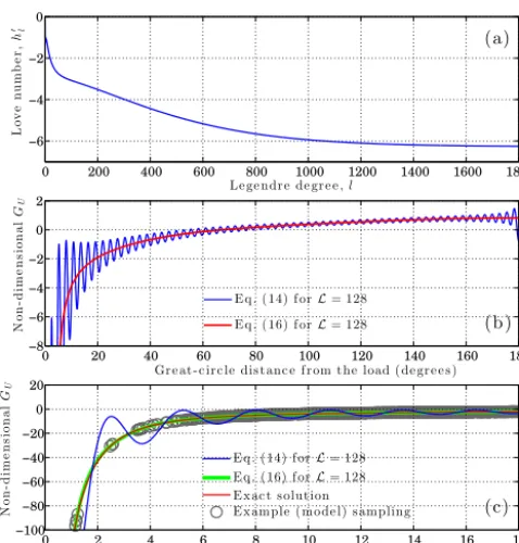
Green’s functions (Eq. 6) that are given in the form of an in-finite sum of Legendre polynomials. Since−kl0decays expo-nentially buth0l approaches very slowly (see Fig. 2a) toward a constant value asl→ ∞, the following discussion focuses on accurate parameterization ofGU. This discussion,
how-ever, equally applies toG8as well.
In contemporary models,GUis evaluated by simply
trun-cating the series at degreeL, such that
GU(α)=
∞ X
l=0
h0lPl(cosα)≈ L
X
l=0
h0lPl(cosα). (14)
Typically, 60<L<600. For L=128, for example, the approximation ofGU is characterized by a systematic noise
Table 1. Constants and parameters used in this study. Solid-earth parameters are taken from Lambeck (1980).
Constant/parameter Symbol Value Unit
Mean rotational velocity of the earth 7.2921×10⁻⁵ s−1
Average density of the earth ρE 5512 kg m−3
Ice density ρI 910 kg m−3
Ocean water density ρO 1000 kg m−3
Chandler wobble frequency (rigid earth) σr 2.4405×10⁻⁷ s−1
Chandler wobble frequency (elastic earth) σr∗ 1.6490×10⁻⁷ s−1
Mean equatorial moment of inertia A 8.0077×1037 kg m2
Polar moment of inertia C 8.0345×1037 kg m2
Gravitational acceleration g 9.81 m s−2
Universal gravitational constant G 6.6738×10⁻¹¹ m3kg−1s−2
Degree 2 tidal (displacement) Love number h2 0.6149 –
Degree 2 tidal (potential) Love number k2 0.3055 –
Secular (fluid) Love number ks 0.942 –
Mean radius of the earth R 6.3710×10⁶ m
same frame is used, for example, for computing gravity fields from the space geodetic satellites.
A much better approximation than Eq. (14) would be the following: we may write (e.g., Schrama, 2005)
GU(α)=
∞ X
l=0
h0lPl(cosα)=h0∞ ∞ X
l=0
Pl(cosα)
+
∞ X
l=0
h0l−h0∞
Pl(cosα), (15)
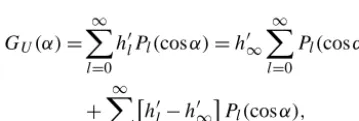
where h0∞ is a constant that is reached asymptotically as l→ ∞. We now assume that h0l=hL0 for all l∈ [L,∞). Since P∞l=0Pl(cosα)=1/[2 sin(α/2)], the above equation
becomes
GU(α)≈
h0L 2 sin(α/2)+
L
X
l=0
h0l−h0LPl(cosα). (16)
ForL=128, this approximation is free from noise (red in Fig. 2b), and virtually the same as the exact solution at least beyond≈1◦from the point of loading (Fig. 2c). The “exact solution” is obtained by summing overL=10 000 (retrieved from http://www.srosat.com/iag-jsg/loveNb.php on 17 Au-gust 2015); the first 1800 terms are shown in Fig. 2a.
SinceGU → −∞asα→0, Eq. (16) cannot be evaluated
at the point of loading, i.e., at α=0. In order to avoid this inherent singularity, we define the loading function (Eq. 2) at the element centroids and evaluate Green’s functions at the vertices so that α >0 for nonzero element size. Let E and
V be the total number of elements and vertices in the mesh (Fig. 1). For each vertexv∈ [1,V], we computeG8andGU
due to unit loads that are centered at the individual elements e∈ [1,E]as follows:
Gve8 GveU
≈ 1
2 sin(αe/2)
1+k0L
h0L
Figure 1. Example of unstructured mesh at earth surface. Both
the (a) Northern and (b) Southern Hemisphere are shown, with continents depicted in cyan. This mesh is generated using Gmsh (Geuzaine and Remacle, 2009), with the BAMG mesh refinement algorithm (Hecht, 2006). The mesh refinement metric employed here is a function of the distance from the nearest coastline.
+ L
X
l=0
kl0−kL0 h0l−h0L
Pl(cosαe)
, (17)
where variables with superscripts ve are matrices of size
V×E, and those witheare vectors of sizeE×1. Figure 2c illustrates how accurately our model samples the exact solu-tion ofGU (i.e., forL=10 000) for an example vertex due
to the nearby elemental unit loads.
Once Gve8 and GveU are computed andLe(t )are given (to be discussed in Sect. 3.3), we may perform the convolution integral (Eq. 7) simply as follows:
8v(t )
Uv8(t )
≈ 3
ρE
1 h
PE e=1Ae
i E X
e=1
gGve8
GveU
Le(t )Ae
, (18)
3.2 Evaluation of3andU3
It is essential to computeL2mn(Eq. 13) andmi(Eqs. 10–11)
prior to evaluating3andU3. Degree 2 SH coefficients of a
loading function can be approximated, according to Eq. (A6), as follows:
L2mn(t )≈
1 h
PE
e=1Ae
i
E
X
e=1
Le(t )Y2emnAe
, (19)
where Y2emn are degree 2 SHs evaluated at elemental cen-troids (θe, λe) of the mesh. Here, it is important to note that SH-based computations on an unstructured mesh are valid for low SH degrees, such asl=2, which have very large sig-nal wavelengths.
The system of non-homogeneous ordinary differential equations appearing in Eq. (10) can be solved for two un-knowns,m1andm2. The solutions are given by
m1(t ) m2(t )
=
cosσr∗t −sinσr∗t sinσr∗t cosσr∗t
c1 c2
+ (20)
− σr
(C−A)
I13(t )−+σr∗ n1(t )cosσr∗t+n2(t )sinσr∗t
I23(t )−+σr∗ n1(t )sinσr∗t−n2(t )cosσr∗t
,
wherec1andc2are constants to be determined from initial
conditions, and
n1(t )
n2(t )
=
Z
I23(t )cosσr∗t−I13(t )sinσr∗t
I13(t )cosσr∗t+I23(t )sinσr∗t
dt. (21) We assume that time-dependent variables may be ex-pressed as the sum of their incremental step changes. For instance,Ii3(t )=PKk=1[δIi3]kH(t−tk), where[δIi3]k is
the incremental step change in moment of inertia over time tk≤t < tk+1induced by the corresponding incremental step
change in applied ice loads and associated sea-level varia-tions (Eq. 13), andH(t−tk)is a Heaviside step function with
magnitude of unity fort≥tkand zero otherwise.
If incremental step changes in parameters are known a pri-ori (or computed) up to and including the Kth time, it is convenient to reset the time so that τ =t−tK. We may
then write, for example, Ii3(τ )=Ii3H(τ ), where Ii3=
PK
k=1[δIi3]k. (For each time interval, we are essentially
treating variables as if these can be expressed using a sin-gle Heaviside step function.) Substitutingtbyτ in Eqs. (20) and (21), a simplification of the latter equation follows
n1(τ ) n2(τ )
= 1 σ∗ r (
I13cosσr∗τ−1
+
I23sinσr∗τ
I13sinσr∗τ−I23cosσr∗τ−1
)
H(τ ). (22) Similarly, the following can be derived from Eq. (11) for m3:
m3(τ )=
c3−
[1+k20] C
1+4
3
[C−A]
C k2 ks
−1
I33H(τ ), (23)
wherec3is yet another constant to be determined from initial
conditions.
Ifmi atτ =0−(i.e., at timet=tK, but just before
impos-ing theKth incremental change) are known, from Eqs. (20) and (23) we may setci=mi(0−). Thenmican be evaluated
for any timeτ ≥0. Settingτ =tK+1−tK, we can compute
mi(0−)and hencecifor the subsequent, i.e.,(K+1)th,
incre-mental change. For the first increincre-mental change, we impose mi(0−)=0 as initial conditions, assuming the initial
equi-librium state of unperturbedω.
Oncemiare computed at a given timet,32mncan be
eas-ily obtained from Eq. (9), and the evaluation of3andU3
becomes fairly straightforward as follows:
3v(t ) U3v(t )
= 2
X
m=0 2
X
n=1
1+k2
h2/g
32mn(t )Y2vmn, (24)
whereY2vmn are degree 2 SHs evaluated at vertices (θv, λv) of the mesh. Recall that these two quantities are key to com-puting the rotational feedback. In this formulation we retain the time dependency as the mass changes directly enter the moment of inertia tensor, which, in turn, drive the solutions ofmi (Eq. 20).
3.3 Evaluation of other variables
As noted earlier, we defineLat the elemental centroids, al-lowing evaluation of the entire set of variables, includingS, at the vertices. SinceLdepends onSitself (Eq. 2), it is nec-essary to mapSv onto the elemental centroids of the mesh, and we do this by simply averaging the correspondingSvfor individual elements. We may now write
Le(t )=ρIHe(t )+ ρO
3 " 3
X
v=1 Sv(t )
#e
Oe, (25)
wherev=1,2,3 are the vertices of theeth (triangular) ele-ment. In order to evaluate the above equation,He(t )andOe
must be provided. We defineOeusing the Generic Mapping
Tools (Wessel et al., 2013) for a set of coordinates (θe, λe) that define the elemental centroids of the mesh.
Similarly, the eustatic terms appearing in Eq. (4) can be evaluated as follows:
E(t ) C(t )
= − R
2
gρO
h PE
e=1AeOe
i 4π 3hPE
e=1Ae
i
E
X
e=1
3gρIHe(t ) ρO
"
3
P
v=1 Cv(t )
#e Oe Ae
, (26)
whereCv=8v+3v−gU8v+U3vand, as indicated by[∗]e
Le ge ndr e de gr e e ,l L o v e n u m b e r, h ′l
0 200 400 600 800 1000 1200 1400 1600 1800 −6
−4 −2 0
Gr e at -c ir c le dis t anc e f r om t he load ( de gr e e s )
N o n -d im e n si o n a l G U
0 20 40 60 80 100 120 140 160 180
−8 −6 −4 −2 0 2
E q . ( 14) f orL= 128
E q . ( 16) f orL= 128
Gr e at -c ir c le dis t anc e f r om t he load ( de gr e e s )
N o n -d im e n si o n a l G U
0 2 4 6 8 10 12 14 16 18
−100 −80 −60 −40 −20 0 20
E q . ( 14) f orL= 128
E q . ( 16) f orL= 128
E x ac t s olut ion
E x ample ( mode l) s ampling
(a)
(b)
(c)
Figure 2. Parameterization of (elastic) solid-earth deformation
caused by surface loading. (a) Load Love numbers,h0l, up to 1800
Legendre degree. Asl→ ∞,h0lconverges slowly toward a constant
value. (b) Non-dimensional Green’s function, GU, computed by
truncating the series atL=128. The conventional approximation
(Eq. 14) produces noise, with greater amplitudes near the loading point. The problem is avoided by using the approximation given by Eq. (16). (c) Demonstration of model ability to accurately
parame-terizeGU. Solutions obtained by truncating the series (according to
Eq. 16) atL=128 are virtually the same as exact solutions (at least
beyond≈1◦from the load), and these are accurately sampled by
our model at an example vertex due to unit loads applied at the el-emental centroids of the mesh (circles in the figure). (See Sect. 3.1 for the explanation of the exact solution.) For comparison, solu-tions associated with Eq. (14) illustrate the ability of contemporary
pseudo-spectral models to parameterizeGU.
Numerical discretization of all components of SLE is now complete, and these can be easily assembled to eval-uate radial displacement of the solid-earth surface (Eq. 5) as Uv(t )=U8v(t )+U3v(t ), change in absolute sea level (Eq. 3) asNv(t )=[8v(t )+3v(t )]/g+E(t )+C(t ), and fi-nally change in relative sea level (Eq. 1) asSv(t )=Nv(t )−
Uv(t ).
3.4 Solution algorithm and model performance
The computational algorithm used in our mesh-based model is similar to that of pseudo-spectral models (Mitrovica and Peltier, 1991) and is as follows: sinceSv(t )must be known while computingLe(t )andSv(t )itself, we employ a recur-sive scheme with an initial solution of Sv(t ) obtained by setting Le(t )=ρIHe(t ) (see Eq. 25). It is then feasible to
iteratively compute Le(t )according to Eq. (25) withSv(t )
obtained from the solution of a previous iteration. We iter-ate the simulation until a metric that quantifies the change in two successive solutions is minimal. It takes only a few itera-tions (typically, five to seven) to converge the solution so that the difference in successive solutions is to within the accept-able accuracy (typically, 5 orders of magnitude smaller than the solution itself). This is the standard algorithm for solving the SLE (e.g., Farrell and Clark, 1976; Mitrovica and Peltier, 1991; Spada and Stocchi, 2007), and does not require further explanation.
Once gravitationally consistent solutions for change in rel-ative sea level,S, are obtained, several useful geodetic ob-servables may be retrieved easily. Of particular interest, we may compute radial displacement of the solid-earth surface, U, from Eq. (5) and change in absolute sea level,N, from Eq. (1). Similarly, we can evaluate the following parameters related to the polar motion of the earth: mass excitation func-tions,χi (fori=1,2), may be computed using the
relation-shipχi =Ii3/[C−A]; positions of the North Pole,(p1, p2),
in the right-handed Cartesian coordinates may be approxi-mated as(p1, p2)≈(m1,m2); and change in the length of
a day,1D, is given by1D= −m3D, whereD≈86 400 s
is the length of a solar day. From some of these solutions, we may also infer other useful geodetic observables, such as changes in absolute gravity and geocentric motion of the earth. These will be further discussed in Sects. 4.2 and 4.3.
Most of our computations are done at the vertices of the mesh. Therefore, we have to mainly deal with vectors of size
V×1. Evaluation of Green’s functions, however, requires that matrices of sizeV×Ebe considered (Eq. 17), and it naturally demands more computer resources. Fortunately, we can com-pute Green’s functions only once at the beginning as a part of the model initialization because these do not evolve as we simulate the model for an assumed elastic earth. For the mesh considered in this study (Fig. 1), which hasV=16 533 and
E=33 102, our Matlab®code takes about 5 min for a serial run in a MacBook Pro (OS X 10.9.5) to compute Green’s functions, and less than a minute to evaluate changes in sea level and associated geodetic parameters caused by instan-taneous melting of a synthetic ice sheet. The employed un-structured mesh has elements of varying size in the range of about [60, 1000] km. We may vary this range, for instance, to capture high-resolution features in particular locations, say around the Amundsen Sea Sector (ASS), yet the computa-tional cost is minimal as noted above as long as the new un-structured mesh consists of similarVandE. The lower limit of element size that our model can handle essentially depends on the degree at which series expansion of Green’s functions (Eq. 17) is truncated. We useL=10 000 for all of our com-putations. Assuming P≈π R/L (Orszag, 1974), where P
denotes the characteristic element size, it implies that our model can capture features of size as small as≈2 km.
an elastic rotating earth. However, for a suitable set of ex-periments, we validate key components of our model by re-producing relevant published results as summarized in Ap-pendix B. We now provide a brief comparison of our mesh model with contemporary pseudo-spectral models in terms of computational efficiency. In the latter models, as noted ear-lier, the SLE is discretized in the SH domain and individual SH coefficients are evaluated. For a chosen spatial resolution,
P, the SH series expansion may be truncated atL≈π R/P, yielding about(π R/P+1)2SH coefficients to be computed. In order to sample the SH signals uniformly over the whole planet, the pseudo-spectral approach also requires that pix-els of equal size be considered. This implies that we must deal with matrices of size≈4π R2/P2×(π R/P+1)2while
evaluating the SLE using pseudo-spectral models. If we are to compute the solutions in spectral formulation, for exam-ple, at 60 km resolution along the coastlines as considered in our mesh-based computation, we must deal with matri-ces of size about 141 685×111 947 (compared to vectors of size 16 533×1 required for our model) that certainly demand huge computer resources. In order to compare the model performance systematically, we consider a pseudo-spectral model that is essentially a Matlab®version of SELEN (Spada and Stocchi, 2007) except the following: (1) the earth’s sur-face is pixelized using MEALPix Toolbox that is a Matlab® version of HEALPix (http://healpix.jpl.nasa.gov/); (2) the solid earth is treated as an elastic sphere; and (3) the SLE includes rotational feedback. This Matlab® version of the model, coded by the authors (unpublished), is tested and val-idated against the original SELEN model for suitable ex-periments. In Table 2, we compare mesh-based and pseudo-spectral models in terms of numerical architecture and com-putational cost. The latter model already demands a large computer resource to capture even a moderate 51 km res-olution. It becomes more cumbersome if we seek to deal with higher wave number features like smaller (kilometer-scale) ice caps and ice fields using pseudo-spectral models, yet there is little degradation in computational efficiency us-ing our mesh-based approach because we can refine the mesh (down to ≈2 km) wherever needed while maintaining the similar numbers of vertices in the mesh.
4 Some geodetic signatures of ice sheets
Of several climate driven phenomena of mass redistribution on the earth’s surface, those related to the cryosphere may be of particular interest. Space-based observations have shown that ice sheets and glaciers expel a large volume of meltwater in an ongoing climate warming (e.g., Shepherd et al., 2012; Gardner et al., 2013), thus directly contributing to the sea-level rise (e.g., Hay et al., 2015). Such trends are likely to per-sist, if not amplify, throughout this century and beyond as in-creased atmospheric and oceanic temperatures are generally predicted for future climate change scenarios (e.g., Bamber
and Aspinall, 2013; Jevrejeva et al., 2014). Here, as an ex-ample model application, we produce computations of some important geodetic signatures associated with the recent evo-lution of contemporary ice sheets. Observed from space or in terrestrial arrays, these signatures provide diagnostic in-formation about strong shifts in climate (e.g., Chen et al., 2013).
4.1 The GRACE data
The twin Gravity Recovery and Climate Experiment (GRACE) satellites are now a way of monitoring and assess-ing earth’s time-varyassess-ing gravity field caused by the climate driven surface mass redistribution and transportation of ma-terials within the earth’s interior (e.g., Wouters et al., 2014). The GRACE data that are now available at an unprecedented resolution of a few hundreds of kilometers have revolution-ized our approach to evaluating, for example, glaciers and ice-sheet mass balance (e.g., King et al., 2012; Ivins et al., 2013; Velicogna and Wahr, 2013; Sasgen et al., 2013) and terrestrial hydrological budget (e.g., Wahr et al., 1998; Swen-son et al., 2003).
The GRACE data are distributed in the form of Stokes co-efficients (Bettadpur, 2012) and, upon standard processing of these SH coefficients, with removal of the mantle GIA signal, we can express the relevant geophysical signals in terms of water height equivalent (WHE). In this analysis, we use GRACE Release-05 Level-2 GSM data products pro-vided by the Center of Space Research, University of Texas at Austin (http://www.csr.utexas.edu/grace/RL05.html). The monthly time series of these data are available up to SH de-gree and order 60, and cover a period from April 2002 to March 2015 (hereafter referred to as the “GRACE period”). There are only partial or no data available for a few months. We fill these data gaps through a simple linear scaling or interpolation between adjacent monthly data as appropriate. We replace degree 1 and degree 2 Stokes coefficients by the values obtained from the analysis of satellite laser ranging (SLR) observations of five passive geodetic satellites (Cheng et al., 2011, 2013a, b). This is particularly important as our computations predict a degree 1 field related to earth’s geo-centric motion and a degree 2 field related to polar motion.
Table 2. Comparison of pseudo-spectral and mesh-based computations of the SLE. We denote element (or pixel) size byP, number of
elements (or pixels) byE, number of vertices byV, and the degree at which (associated) Legendre series is truncated byL. (Vis not relevant
for the pseudo-spectral approach.)
Model E V P(km) L Initial timea SLE timeb Processorc
Mesh-based 33 102 16 553 60–1000d 10 000 5 min <1 min Serial
12 288 – 204 98 <1 min <1 min Serial
Spectral 49 152 – 102 196 20 min 10 min Serial
196 608 – 51 392 2 h 4 h Parallel
aIt is the model initialization time. For pseudo-spectral models, most of this time is required to compute SHs that would be of size
E×(L+1)2. Our model mainly utilizes this time to compute Green’s functions, which are of sizeV×E.
bIt is the CPU time required to solve the SLE following instantaneous melting of a hypothetical ice sheet. Pseudo-spectral models once again deal with matrices of sizeE×(L+1)2. Our model mostly deals with vectors of sizeV×1.
cBoth pseudo-spectral and mesh-based models are coded in Matlab®and simulated in a MacBook Pro (OS X 10.9.5). We employ the Parallel Computing Toolbox™of Matlab®with four local workers in parallel runs. Serial runs use a single worker. dOur model has variable element size. ForL=10 000, in principle, it can capture features of size as small as≈2 kmat minimal computational cost as listed above (provided that the new unstructured mesh consists of similarVandE).
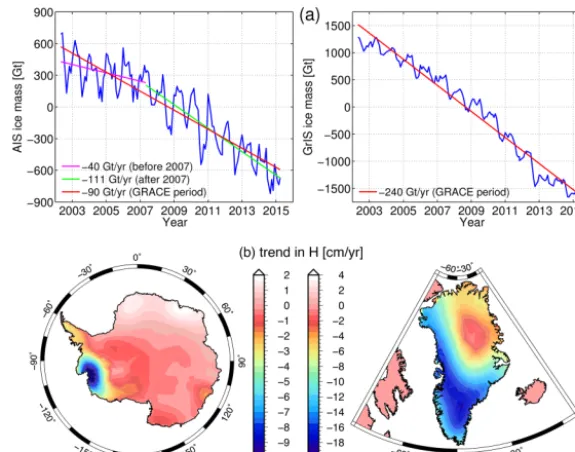
that we employ a GIA computed by A et al. (2013) and select a rescaling such that the linear trends in ice mass loss from the Antarctic Ice Sheet (AIS) and Greenland Ice Sheet (GrIS) during the GRACE period are −90 and−240 Gt yr−1,
re-spectively. Throughout, we apply a Gaussian smoothing with a 300 km radius. This smoothing radius may be large enough to filter the short-wavelength noise, yet small enough to re-tain the actual geophysical signals, and is in the range of typ-ical values recommended for variety of applications (Wahr et al., 1998; Swenson et al., 2003).
The temporal and spatial trends in the final products of the AIS and GrIS mass balance are shown in Fig. 3. The am-plitudes of temporal variability are higher for the AIS, im-plying the large seasonal mass turnover there, but it could also be due to large signal amplitudes of the GIA model used (A et al., 2013). A kink is apparent in the AIS data (Fig. 3a); the ice sheet has lost more mass (−111 Gt yr−1) since 2007 than during the early period (−40 Gt yr−1). On the other hand, the GrIS was losing the mass more steadily with a little seasonal turnover, but at a much greater pace (−240 Gt yr−1). Spatial distributions of the (linear) mass
bal-ance trend are shown in Fig. 3b. The figure suggests that the AIS was mostly losing the mass from the ASS at a large rate (dH /dt≤ −10 cm yr−1), and also from the Peninsula and Wilkes Land at a more modest rate. Note that the AIS has also gained mass in a few locations; there are clear signals of mass gain (at a rate of about 2 cm yr−1) in the northern East Antarctic Ice Sheet (EAIS). The GrIS lost mass at a much greater pace of about−20 cm yr−1, mainly from the south-eastern sector during the first half of the GRACE period, but losses also expanded toward the west later on. Figure 3b also suggests small mass changes in the north and interior of the GrIS during the GRACE period. All these features are gen-erally consistent with other published solutions, for both AIS and GrIS (e.g., Velicogna and Wahr, 2013). However, it is im-portant to note that our primary goal here is to demonstrate
the predictive capabilities of our mesh-based model rather than computing precise mass budget solutions for the polar ice sheets. In Sect. 5 we describe some application of the methods to high-resolution ice-sheet models.
4.2 Sea level and other variables
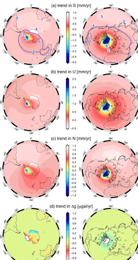
The monthly time series ofH (θ, λ, t )for both ice sheets are obtained from the GRACE data as discussed above. We force loading of the model by these mass balance solutions for the two major ice sheets. Our model computes monthly solu-tions for relative sea level,S, radial displacement of solid-earth surface,U, and perturbation in absolute sea level,N. Figure 4 summarizes these solutions for a combined forc-ing of ice sheets, where we show the linear trends in vari-ables obtained by fitting the corresponding monthly solu-tions in a least-square sense. Figure 4a depicts the trend in S with the following key features: a large rate of sea-level drop (dS/dt≤ −3.0 mm yr−1) with large wavelengths around the GrIS; the same, but with relatively smaller wave-lengths around the ASS; and a moderate rate of sea-level rise (1.5 mm yr−1) in the northern EAIS. The blue contours represent the global mean rate (GMR) of relative sea-level rise with a magnitude of about 0.91 mm yr−1. The corre-sponding values for the AIS and GrIS are about 0.25 and 0.66 mm yr−1, respectively. In the regions enclosed by these contours, sea level either falls or remains unchanged or rises more slowly than the GMR. In the exterior regions, on the other hand, sea level rises at a higher pace than the GMR.
Figure 3. Summary of the GRACE data used in this study. (a) Ice mass change in the AIS and GrIS from April 2002 to March 2015. (b) Spatial distribution of rate of change in ice thickness, averaged over the GRACE period. See Sect. 4.1 for a detailed discussion of the
GRACE data processing.
Table 3. Location of selected tide gauge stations, with Global Sea
Level Observing System (GLOSS) ID.
ID∗ GLOSS ID Location Latitude Longitude
N1 28 Male, Maldives 4.17◦N 73.5◦E
N2 86 Mera, Japan 34.55◦N 139.49◦E
N3 108 Honolulu, HI 21.30◦N 157.87◦W N4 158 San Francisco, CA 37.80◦N 122.47◦W N5 332 Virginia Keys, FL 25.73◦N 80.16◦W N6 229 Reykjavik, Iceland 64.15◦N 21.93◦W
N7 241 Newlyn, UK 50.10◦N 5.55◦W
S1 13 Durban, South Africa 29.88◦S 31.03◦E S2 129 Bluff, New Zealand 46.60◦S 168.35◦E S3 195 Rio de Janeiro, Brazil 22.90◦S 43.17◦W S4 95 Syowa, Antarctica 69.00◦S 39.60◦E S5 278 Casey, Antarctica 66.28◦S 110.53◦E S6 – Pine Is Glacier, Antarctica 75.17◦S 100.00◦W S7 188 Rothera, Antarctica 67.57◦S 68.13◦W
∗ID has the following format:X0, whereX=N or S (for the Northern and Southern Hemisphere) and 0=1, . . .,7(see Fig. 4a for their position on the global map).
surface uplift is predicted to occur at a relatively large rate (dU/dt≥2.5 mm yr−1) around the ASS and GrIS, and
sub-sides at a rather moderate rate of−0.5 mm yr−1around the
northern EAIS. The trend inN shows much greater variabil-ity in space (Fig. 4c). Here the computation is performed in the CM reference frame and the corresponding Green’s function does not change monotonically (unlike those forS andU) as a function of great-circle distance from the load-ing point. Note in Fig. 2b howGU, for example, increases
monotonically as the evaluation point moves away from the load. The predicted change in absolute sea level drops at
a rate of dN/dt≤ −1.0 mm yr−1around the ASS and GrIS,
while a rise is predicted at a similar rate in the northern EAIS and the northern Pacific. Generally speaking, the relative sea level, sea surface height and solid-earth deformation are lin-early related to each other (Eq. 1). Therefore, sea-level drop is generally accompanied by the earth surface uplift and sea surface fall, and sea-level rise is by the earth surface subsi-dence and sea surface rise.
It may be useful to evaluate the corresponding changes in absolute gravity (gravity anomaly or disturbance), because this geodetic variable may be measured directly using abso-lute gravimeters (e.g., James and Ivins, 1998; Crossley et al., 2012) and space geodetic satellites. It may be possible to compute this variable on the same computational mesh as we use for solving the SLE, but it is more readily estimated from the solutions ofNin the SH domain. Here we evaluate gravity anomaly,1g, that could be measured by a gravimeter on the earth’s surface as follows (Lambeck, 1980):
1g(θ, λ, t )=4π
3 GρE
∞ X
l=0
l X
m=0 2
X
n=1
(l−1)Nlmn(t )Ylmn(θ, λ), (27) whereNlmn are the SH coefficients ofN. The linear trend
Figure 4. Some important geodetic signatures of ice sheets
dur-ing the GRACE period. Rates of change in (a) relative sea level,
(b) solid-earth deformation, (c) absolute sea level, and (d)
abso-lute gravity. (Notice the different scale and color order in the color bars.) These results are obtained by linearly fitting the correspond-ing monthly solutions in a least-square sense. The blue contours in
(a) represent the trend in the global mean value, with magnitude
dS/dt=0.91 mm yr−1. Annotations are supplied for 14 locations
in (a) (see Table 3 for their description).
An interesting exercise is to compare the relative contri-bution of individual ice sheets to the total sea-level change. (Total sea-level change, in the context here, is due to the combined mass evolution of both AIS and GrIS.) For such analysis, we select 14 representative tide gauge stations, half of which are located in the Northern Hemisphere. The
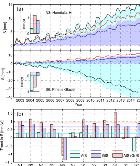
de-scriptions of these sites are given in Table 3 and their co-ordinates on the global map are shown in Fig. 4a. For two representative sites (one for each hemisphere), Fig. 5a shows the explicit evolution of sea-level change and the relative contribution of AIS and GrIS. In Honolulu, the total sea level rises faster (black line in the figure) than the GMR (red line) throughout the GRACE period. The GrIS contribu-tion at this site is higher (light blue fill) than its contribucontribu-tion to the global mean value (blue line). The AIS influence at this site is similar. This is summarized in the figure inset, in which we compare the average trends in sea-level variation: the local contributions of GrIS (dS/dt=0.82 mm yr−1) and AIS (0.33 mm yr−1) are both greater than the corresponding GMRs (i.e., 0.66 and 0.25 mm yr−1, respectively), thus re-sulting in a much greater pace of local sea-level rise in Hon-olulu (1.15 mm yr−1) than the GMR (0.91 mm yr−1). By
con-trast, the total sea level falls at a rapid pace in the Pine Island Glacier (−2.88 mm yr−1) despite the positive and larger than
global mean contribution of GrIS (0.82 mm yr−1), and it is mainly due to the local gravitational loss (Fig. 4d) associated with a strong loss in ice mass from the ASS (Fig. 3b).
Figure 5b summarizes a similar comparison for dS/dt at other tide gauge stations (see Table 3 and Fig. 4a). Although the figure is self-explanatory, we make brief remarks on some interesting features. On both the western coast (San Fran-cisco; N4) and the eastern coast (Virginia Keys; N5) of the continental United States, contributions of AIS are greater and those of GrIS are smaller than the corresponding GMRs. Their combined effects, however, are somewhat contrasting: the pace of local sea-level rise (0.93 mm yr−1) is slightly higher than the GMR at San Francisco, and the opposite is true for Virginia Keys, where sea level rises at a rather mod-est rate of 0.82 mm yr−1. Greatly contrasting rates are
pre-dicted at two closely located places, namely Reykjavik (N6) and Newlyn (N7). Since the AIS contributions are similar at both sites, differing signatures in total sea-level change are due to the GrIS: the ice sheet has a strong negative contribu-tion at Reykjavik, causing the total sea level to drop at the great rate of−1.07 mm yr−1. Its contribution at Newlyn, on the other hand, is minimal, and therefore the total sea level there rises much more slowly than the GMR (0.34 mm yr−1). Note that there are other interesting comparisons such as be-tween the eastern (Casey; S5) and western (Rothera; S7) lim-its of the AIS. At Casey in the EAIS, the AIS contribution is minimal and the total sea-level rise (0.67 mm yr−1) is mainly due to the GrIS. However, at Rothera, both ice sheets have similar contributions but opposite signs, thus resulting in a virtually stagnant sea level (0.05 mm yr−1). In the end, it is
also worthwhile reporting the overwhelmingly great pace of sea-level rise (1.54 mm yr−1) at Syowa in the northern EAIS (S4). The AIS contribution is large there, mainly due to the enhanced gravitational pulling (Fig. 4d) associated with the local mass gain (Fig. 3b).
flex-Tide gauge station ID
Trend in S [mm/yr]
N1 N2 N4 N5 N6 N7 S1 S2 S3 S4 S5 S7 −1.5
−1 −0.5 0 0.5 1 1.5
AIS GIS AIS+GrIS Year
S [mm]
2003 2004 2005 2006 2007 2008 2009 2010 2011 2012 2013 2014 2015 −40
−30 −20 −10 0 10
S [mm]
0 5 10 15
mm/yr
−4 0
mm/yr
0 1
(b) (a)
S6: Pine Is Glacier N3: Honolulu, HI
Figure 5. Magnitudes and trends of sea-level change at 14 selected
locations. (See Table 3 for their description and Fig. 4a to locate their position on the global map.) (a) Change in relative sea level over time at two representative sites. Average rates of relative sea-level change are also shown in the insets. (b) Rate of change in relative sea level, averaged over the GRACE period, at 12 other locations. Cyan and blue colors (both fill and line) represent the contribution from the AIS and GrIS, respectively. The combined contributions of ice sheets are shown in red. Black lines in Fig. 5a represent the local values and all others denote the global mean val-ues.
ible FE mesh system. In the section that follows we apply those model predictive features to two important geodynam-ical observables associated with space geodesy: polar motion and geocentric motion of the earth.
4.3 Polar motion and geocentric motion
The redistribution of mass on the earth’s surface (Eq. 2) ex-cites changes in the position of the rotational spin axis with respect to fixed positions in the crust. This is also known as changes in “earth orientation”, or is commonly known as po-lar motion (Lambeck, 1980), and has important observational ties to the mass imbalance of the earth’s two great ice sheets (Douglas et al., 1990). The GMR of sea-level rise caused by ice sheets is roughly 1 mm yr−1since about 2005 (Shepherd et al., 2012). If rates increase during the next 80–100 years, sufficient to reach the upper end of the estimate of Jevrejeva et al. (2014) for 2100 (≈180 cm), then it will be important to have the state-of-the-art data assimilating ice-sheet
mod-els, such as ISSM, incorporate such a profoundly fundamen-tal observable. Here we compute some important attributes of polar motion induced by contemporary ice sheets and as-sociated sea-level changes during the GRACE period.
Figure 6a and b shows 3-D plots for the monthly posi-tion of the North Pole. Complex interacposi-tions between the near-annual forcing and Chandler (433-day period) wobble results in a net polar wobble with varying amplitude. This can be seen in the figures for both ice sheets. While wob-bling around the mean rotational axis, the pole also drifts away from its initial position, as indicated by trend lines in the figures. A kink in the drift direction is apparent for the AIS in about 2007, which may be linked to a similar feature observed in mass evolution of the ice sheet (see Fig. 3a).
In order to predict polar drift from our mesh-based computational framework, we evaluate classic mass exci-tation functions, χ1 andχ2, associated with individual ice
sheets (Fig. 6c) and the corresponding annual pole positions (Fig. 6d). The North Pole in Fig. 6d represents that of year 2002. The mass loss in the GrIS yields positiveχ1and
neg-ativeχ2in the employed right-handed Cartesian system,
im-plying that the general drift direction is toward the fourth quadrant defined byx1>0 andx2<0 (see Fig. 6d). Sinceχ1
andχ2are on a similar order of magnitudes, the GrIS induced
drift is directed toward the ice sheet itself along≈40◦W lon-gitude. On the other hand, the combination of rapid mass loss in the ASS and mass gain in the northern EAIS yields posi-tive excitation functions, thus causing the North Pole wander vector to be directed toward a Eurasian≈60◦E longitude. Since the AIS and GrIS operate in-phase for χ1 and
out-of-phase forχ2, their combined effects would amplify the
former excitation function and shrink the latter one. Conse-quently, the pole would be drifting along≈15◦W longitude during the GRACE period as shown in Fig. 6d.
These predictions are generally consistent with the re-port by Chen et al. (2013): glaciers and ice sheets explain a large fraction of observedχ1during 2005–2011, but their
contributions toχ2 are minimal. We find dχ1/dt=2.87±
0.15 mas yr−1 for the same period, which is approximately half the trend attributed by Chen et al. (2013) to glaciers and ice sheets. Large rates of mass loss from other glaciated re-gions such as the high-altitude Himalayas (Gardner et al., 2013) may explain the discrepancy, although more rigorous effort is needed to justify this. Despite the minimal collective contributions of glaciers and ice sheets to the observed trend inχ2, it is important to highlight the significant role that the
AIS is playing to counter the GrIS induced negativeχ2(see
Fig. 6c). Rapid mass loss from the ASS, aided by the mass gain in the northern EAIS, is responsible for drifting the pole along≈15◦W longitude, which would otherwise be head-ing the GrIS. Observations of further eastward motion of the pole (along≈15◦E longitude; Fig. 6d) may be explained by mass transport and other excitations unrelated to ice sheets.
mo-Figure 6. Polar motion during the GRACE period. Monthly pole positions (with respect to April 2002),(p1, p2), excited by (a) AIS and
(b) GrIS mass loss in the right-handed coordinate system(x1, x2)(see d). Red lines show the average drift directions. A kink is apparent
for the AIS. (c) Mass excitation functions, χ1and χ2, associated with individual ice sheets. (d) Annual pole positions, after removing
Chandler wobbles, with respect to the 2002 position. For comparison, the observed long-term (green arrow; Mitrovica et al., 2006) and
recent (2005–2011; blue arrow; Chen et al., 2013) drift directions are also shown. Note that 1 mas≈3.09 cm.
tion of the earth. While observationally more elusive than polar motion, this is a fundamental parameter important to global reference frames. The geocentric motion is caused by the shift in relative position between the CM of the earth sys-tem and the center of figure (CF) of the solid-earth surface, and this information is essential to reconcile the geodetic data that are tracked from the ground stations using abso-lute gravimeters and also from the passive geodetic satellites using SLR. Let the CM-CF shift be denoted by the position vectorXi (fori=1,2,3) in the right-handed Cartesian
sys-tem. The components of this vector can be computed from the degree 1 SH coefficients of a gravitationally consistent loading function (Eq. 2) as follows (e.g., Wu et al., 2006): Xi(t )=
√
3 ρE
1−h
0
1+2l
0
1
3
[L111(t )δ1i+L112(t )δ2i
+L101(t )δ3i], (28)
whereδ1i,δ2i, andδ3iare the Kronecker deltas, andl01is the
degree 1 load Love number, just like h01andk10, and in the employed CM reference frame is on the order l10 = −0.89 (Blewitt, 2003).
The ice-sheet induced components of X during the GRACE period are plotted in Fig. 7. Since both ice sheets are located near the poles (i.e., with small |xi| for i=1,2
and large|x3|), their individual contributions to the CM-CF
shift are naturally larger forX3, which is associated with a
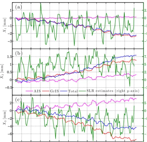
degree 1 zonal harmonic. However, the ice sheets have sec-ular trends in this component of geocentric motion that op-pose one another. This opposition mutes their combined sig-nal (Fig. 7c), predicting a gradual shift toward the South Pole at a rate of−0.44±0.03 mm yr−1. Both seasonal amplitudes and secular trends in horizontal components of the geocentric motion, i.e.,X1andX2, are quite minimal, compared with
the corresponding solutions inferred from the SLR observa-tions (Cheng et al., 2013b), despite the in-phase functioning of ice sheets for the latter component. Incorporation of de-gree 1 predictions into ice-sheet models such as ISSM will be important for considering geodetic reference frame stabil-ity, but it is unlikely to be relegated to the status of a data as-similation parameter due to problems with inferring decadal timescale CM-CF drift (Ries, 2013), especially when com-pared to other global space geodetic observables.
5 Sea-level fingerprints of high-resolution ice-sheet forcing
reso-X
1
[m
m
]
−3 −2 −1 0 1
−7.5 −5 −2.5 0 2.5
X
2
[m
m
]
−0.5 0 0.5 1 1.5
−2.5 0 2.5 5 7.5
A I S Gr I S Tot al SLR e s t imat e s ( r ighty-ax is )
Ye ar
X
3
[m
m
]
2002 2004 2006 2008 2010 2012 2014 2016 −6
−4 −2 0 2
2002 2004 2006 2008 2010 2012 2014 2016 −15 −10 −5 0 5
(a)
(b)
(c)
Figure 7. Geocentric motion during the GRACE period. The
CM-CF shift, with respect to the April 2002 position, along the (a)x1,
(b) x2, and (c)x3 directions in a right-handed Cartesian system.
(See Fig. 6d for a positive sense of horizontal axes; the vertical axis,
x3, is positive out of the North Pole.) Note that different scales are
used (in the rightyaxis) for the SLR-based estimates (Cheng et al.,
2013b).
lution (on the order of 250–350 km), allowing us to consider a relatively coarse mesh (with smallest elements on the order of 60 km). However, one of the major goals of ISSM-SESAW is to be able to resolve the kilometer-scale source of earth’s time-varying surface mass transport (e.g., fast-flowing outlet glaciers, and rapid changes in grounding line position) and project it globally. In order to demonstrate this, we provide an example computation of sea-level fingerprint associated with high-resolution modeling of polar ice sheets.
We model the dynamics of polar ice sheets over high-resolution mass conserving beds (Morlighem et al., 2014, and personal communication). We mesh the ice sheets anisotropically from 50 km (AIS) and 15 km (GrIS) at the ice divide to 3 and 1 km in fast-flowing regions, respectively, with respective ice shelves meshed at 9 and 1 km. These meshes comprise a total of 102 308 (AIS) and 93 039 el-ements (GrIS). For both ice sheets, we perform a 200-year control run using a 2-D shelfy-stream approximation (MacAyeal, 1993) for ice-flow mechanics. The models are initialized from steady state using basal friction inversion (Larour et al., 2012; Schlegel et al., 2015) and present-day InSAR surface velocities (Rignot et al., 2011). The models are initially relaxed to thermal steady state as well (Seroussi et al., 2013). The model forcings include a surface climatol-ogy provided by Regional Climate Model RACMO2.3 (Et-tema et al., 2009) averaged during 1979–2010, and melt rates
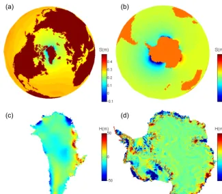
under Antarctic ice shelves obtained from mean annual sim-ulation of ECCO (Estimating the Circsim-ulation and Climate of the Ocean) over 1992–2012 (Heimbach, 2008). The global sea-level model comprises the actual high-resolution meshes of both ice sheets, and is anisotropically adapted from 1 km in the highest-velocity areas of GrIS to 2000 km in the middle of the Pacific Ocean, for a total of 292 262 elements. Coast-lines are resolved with the Generic Mapping Tool (Wessel et al., 2013), and the mesh itself is generated using Gmsh (Geuzaine and Remacle, 2009). We compute relative sea level on this global mesh by forcing ISSM-SESAW with high-resolution ice thickness change over a 200-year control run on both polar ice sheets. Solutions are shown in Fig. 8. Large negative changes in sea level are evident around both ice sheets, symptomatic of the overall loss of mass from both AIS and GrIS during the control runs.
These solutions are obtained by running ISSM-SESAW on NASA’s Pleaides supercomputer. Due to the intensive na-ture of the convolution operation (i.e., a load defined at every elemental centroid contributes to sea level evaluated at ev-ery vertex of the mesh), a low-latency bandwidth network is required to distribute solutions across the network in a dense pattern. Pleaides has an InfiniBand®interconnect, with all nodes connected in a partial hypercube topology, which makes this operation possible. Scaling is highly dependent upon the convolution loop, which needs to be carried out in a fragmented way, to space out the distribution of values across the cluster. This operation is CPU dependent, but is also highly limited by the interconnect speed. Without the discretization of SLE that operates on a flexible unstructured mesh system (presented in this paper) and use of a massively parallelized and fully scalable capability of ISSM-SESAW, such a high-resolution computation of relative sea level and associated global geodetic observables would have been vir-tually impossible.