www.geosci-model-dev.net/9/1803/2016/ doi:10.5194/gmd-9-1803-2016
© Author(s) 2016. CC Attribution 3.0 License.
Coupling aerosol optics to the MATCH (v5.5.0) chemical transport
model and the SALSA (v1) aerosol microphysics module
Emma Andersson1and Michael Kahnert1,2
1Department of Earth and Space Sciences, Chalmers University of Technology, 41296 Gothenburg, Sweden 2Swedish Meteorological and Hydrological Institute, 60176 Norrköping, Sweden
Correspondence to: Michael Kahnert (michael.kahnert@smhi.se)
Received: 3 November 2015 – Published in Geosci. Model Dev. Discuss.: 21 December 2015 Revised: 21 April 2016 – Accepted: 25 April 2016 – Published: 12 May 2016
Abstract. A new aerosol-optics model is implemented in which realistic morphologies and mixing states are assumed, especially for black carbon particles. The model includes both external and internal mixing of all chemical species, it treats externally mixed black carbon as fractal aggregates, and it accounts for inhomogeneous internal mixing of black carbon by use of a novel “core-grey-shell” model. Simulated results of aerosol optical properties, such as aerosol optical depth, backscattering coefficients and the Ångström expo-nent, as well as radiative fluxes are computed with the new optics model and compared with results from an older optics-model version that treats all particles as externally mixed ho-mogeneous spheres. The results show that using a more de-tailed description of particle morphology and mixing state impacts the aerosol optical properties to a degree of the same order of magnitude as the effects of aerosol-microphysical processes. For instance, the aerosol optical depth computed for two cases in 2007 shows a relative difference between the two optics models that varies over the European region between−28 and 18 %, while the differences caused by the inclusion or omission of the aerosol-microphysical processes range from−50 to 37 %. This is an important finding, sug-gesting that a simple optics model coupled to a chemical transport model can introduce considerable errors affecting radiative fluxes in chemistry-climate models, compromising comparisons of model results with remote sensing observa-tions of aerosols, and impeding the assimilation of satellite products for aerosols into chemical-transport models.
1 Introduction
and assess the level of morphological detail that might be re-quired in aerosol-optics models coupled to CTMs.
A main difficulty is that aerosol particles in nature can have a high degree of morphological complexity. For in-stance, mineral dust particles can have irregular shapes, small-scale surface roughness, and inhomogeneous miner-alogical composition (e.g. Nousiainen, 2009). Black car-bon particles suspended in air have fractal-aggregate shapes (e.g. Jones, 2006) that can be coated by weakly absorb-ing liquid-phase components that condense onto the aggre-gates as they age in the atmosphere (e.g. Adachi and Buseck, 2008). Volcanic ash particles are composed of crustal ma-terial in which multiple air vesicles may have been trapped during the generation of the particles. In aerosol-optics mod-els one has to make a choice what level of morphological detail is necessary and affordable. A detailed discussion of this question can be found in Kahnert et al. (2014).
In environmental modelling practical and computational constraints often force us to invoke drastically simplifying assumptions about aerosol morphology. For instance, one frequently computes aerosol optical properties based on the assumption that all chemical aerosol components are con-tained in separate particles (externally mixed), and that each such particle can be approximated as a homogeneous sphere. As pointed out in Kahnert (2008) and Benedetti et al. (2009), this approach is highly attractive from a practical point of view, because the aerosol optical observation operators, which map mixing ratios to radiometric properties, become linear functions of the mixing ratios of the different chemical species. A linearization of the observation operator is a pre-requisite for most of the commonly used data-assimilation methodologies, such as the variational method (e.g. Kahnert, 2008; Benedetti et al., 2009). However, such approximations can also introduce substantial errors. In the remote sensing community awareness of this problem has been growing over the past 1–2 decades. As a result, one has developed retrieval methods for desert dust aerosol particles that are based on spheroidal model particles (e.g. Dubovik et al., 2006), which can mimic the optical properties of mineral dust particles bet-ter than homogeneous spheres (Kahnert, 2004; Nousiainen et al., 2006). In chemical data assimilation, the problem is still treated rather negligently. A few assimilation studies ac-count for internal mixing (where several aerosol components can be contained within one particle) of different chemical components (e.g. Saide et al., 2013). But the particles are still assumed to be perfectly homogeneous spheres. To the best of our knowledge there are currently no aerosol optical observation operators in chemical transport models that take complex morphological properties of aerosol particles such as non-sphericity or inhomogeneous internal structure into account.
This study describes the coupling of two different aerosol-optics models to a regional CTM. One aerosol-optics model is based on the simple external-mixture and homogeneous-sphere ap-proximations. The second model takes both external and
in-ternal mixing of aerosol components into account. Also, it employs morphologically more realistic models for black carbon particles. Although black carbon contributes, on av-erage, only some 5 % to the mass mixing ratio of particulate matter over Europe, it can have a significant global radiative warming effect. Previous theoretical studies on the optical properties of black carbon particles suggest that the use of homogeneous-sphere models can introduce substantial errors into the absorption cross section and single scattering albedo of such particles (e.g. Kahnert, 2010a; Kahnert et al., 2013). Also, the largest mixing-state sensitivity in both regional and global radiative fluxes comes from black carbon according to Klingmüller et al. (2014).
The main goal of this study is to assess the impact of aerosol morphology and mixing state on radiometric quan-tities and radiative forcing simulated with a chemical trans-port model. To this end we compare the two optics models, and we gauge the significance of morphology by comparing the differences in the optics model output to other sources of error. As a gauge we use the impact of including or omitting aerosol microphysical processes; this provides us with a ref-erence which is generally agreed to have a significant effect on aerosol transport models (Andersson et al., 2015; Kokkola et al., 2008).
The CTM, its aerosol microphysic and mass transport set-ups, and the aerosol-optics models are described in Sect. 2. There we also explain the methodology we employ for com-parison of the optics models. In Sect. 3 we present and dis-cuss computational results for selected cases and for sev-eral radiative and optical parameters. Concluding remarks are given in Sect. 4.
2 Model description and methods
2.1 General considerations and terminology
inter-nal mixture. There are two types of interinter-nal mixtures. If e.g. hydrophilic liquid-phase components mix with each other, one can obtain a homogeneous internal mixture of different chemical species. On the other hand, condensation of gas-phase species onto non-soluble primary particles or cloud processing of aerosol particles can result in liquid-phase ma-terial coating a solid core of e.g. mineral dust or black carbon. We refer to the latter as an inhomogeneous internal mixture. Aerosol populations in nature are often both externally and internally mixed, i.e. they contain particles that are composed of a single chemical species as well as other particles that are composed of different chemical species, which can be homo-geneously or inhomohomo-geneously internally mixed.
Aerosol optical properties are strongly dependent on not only the size and chemical composition, but also on the mix-ing state, shape, and internal structure of particles. Therefore, before explaining the aerosol-optics model, we first need to briefly describe the kind of information that can be provided by the aerosol transport model. In particular, we need to un-derstand the level of detail with which the size distribution, size-dependent chemical composition, and the mixing state of the aerosol particles can be computed in a large-scale model.
2.2 Aerosol transport modelling with MATCH
As a regional model we employ the Multiple-scale At-mospheric Transport and CHemistry modelling system (MATCH), an offline Eulerian model developed by the Swedish Meteorological and Hydrological Institute (Ander-sson et al., 2007). For this study we have set up the MATCH model over the European domain with a 0.4×0.4◦ horizon-tal resolution and a rotated latitude–longitude grid, covering about 34◦longitude and 42◦latitude. The model has 40 verti-calηlayers with varying thicknesses depending on the topog-raphy, and it extends up to about 13 hPa. The meteorological input comes from the HIRLAM (HIgh-Resolution Limited Area Model) numerical weather-prediction model (Unden et al., 2002).
The MATCH model allows us to choose between two aerosol model versions, a simpler mass-transport model, and a more sophisticated aerosol dynamic transport model. 2.2.1 Mass transport model
A simple version of the MATCH CTM, which we refer to as the “mass-transport model”, neglects all aerosol dynamic processes. It contains a photochemistry model that com-putes mass concentrations of secondary inorganic aerosols (SIAs), which are formed from precursor gases. The SIA fraction of aerosol particles consists of ammonium sulfate ((NH4)2SO4), ammonium nitrate (NH4NO3), other particu-late sulfates (PSOx), and other particulate nitrates (PNOx). The mass transport model furthermore contains a sea-salt module that computes NaCl emissions based on the
param-eterizations described in Mårtensson et al. (2003) and Mon-ahan et al. (1986). More details on the MATCH photochem-istry model can be found in Robertson et al. (1999) and Andersson et al. (2007); the MATCH sea-salt model is de-scribed in Foltescu et al. (2005). The mass transport model also contains a simple wind-blown dust model and a mod-ule for transport of primary particulate matter (PPM), i.e. aerosol particles other than sea salt and wind-blown dust that are emitted as particles, rather than being formed from gas precursors. The size bins in the PPM model are flexible. In the current model set-up the sea-salt and PPM models were run for four size bins as shown in Table 1. We used gridded EMEP PPM emission data for the year 2007 in conjunction with black carbon (BC) and organic carbon (OC) emission data by Kupiainen and Klimont (2004, 2007). The latter pro-vide BC and OC emissions per country and emission sector. We distributed these among the grid cells in the model do-main according to the EMEP PPM gridded emissions. Thus, the BC and OC emissions vary among grid cells in accor-dance with the EMEP PPM emissions, while the sum of all BC and OC emissions over all grid cells per country and emission sector agrees with the corresponding BC and OC emissions, respectively, reported in Kupiainen and Klimont (2004, 2007). The remaining emissions (PPM-BC-OC) in each grid cell are interpreted as dust particles. The primary-particle emissions are distributed among the size bins; dur-ing atmospheric transport they remain chemically and dy-namically inert in the model. Thus no chemical transforma-tion, mixing processes with other compounds, or other size-transformation processes are included in the model. The SIA components are given as total mass concentrations without any information about their size distribution. In the optics model a fixed size distribution is assumed to assign the total SIA mass to the four size bins. Water adsorption by particles is computed in the optics model as described in Sect. 2.3.1. 2.2.2 Aerosol microphysics module – SALSA
Table 1. Size bins (characterized by the radiusr) and chemical species in the MATCH mass transport model (Andersson et al., 2007). The labels “p” and “s” refer to primary emitted particles and secondary particles generated from gas precursors.
Size Other Other Other
bin r(nm) OC BC Dust PPM NaCl (NH4)2SO4 NH4NO3 PSOx PNOx
1 10–50 p p p p s s s s
2 50–500 p p p p s s s s
3 500–1250 p s s s s
4 1250–5000 p p p p p s s s s
Table 2 shows the current model set-up with the num-ber and range of the size bins. As is evident from this ta-ble, MATCH-SALSA accounts for both internally and exter-nally mixed aerosol particles. In total, there are 20 different size bins in MATCH-SALSA, each one of them represent-ing a particle size range (volume-equivalent radius,r), mix-ing state, and composition. Some size bins have the same size range, but different mixing states and/or compositions. For instance, size bins 12, 15, and 18 describe the same size range (350–873 nm), but different internal mixtures of vari-ous species. Similarly, bins 4 and 8 have the same size range (25–49 nm), but one describes an internal mixture, the other an external mixture of aerosol species.
As in the mass-transport model, “other PPM”, i.e. primary particles other than BC and OC, are interpreted as dust parti-cles. Note that water is not directly calculated as a prognostic variable in MATCH-SALSA. Rather, it is a diagnostic vari-able computed in the MATCH-optics model as explained in Sect. 2.3.2. The table merely indicates which size bins are assumed in the optics model to be internally mixed with ad-sorbed water. A more detailed description of the MATCH-SALSA model can be found in Andersson et al. (2015). 2.3 Aerosol-optics modelling
Aerosol-optics models coupled to a CTM have to make con-sistent use of the information provided by the CTM, while invoking assumptions on optically relevant parameters that are not provided by the CTM. The parameters that influence the particles’ optical properties are
– the aerosol size distribution;
– the refractive index of the materials of which the aerosol particles are composed; and
– the morphology of the particles.
Morphology refers to both the overall shape of the particle, and, in case of inhomogeneously mixed particles, the varia-tion of the refractive index inside the particle.
The information provided by the CTM depends on the level of detail in the process descriptions. In the MATCH mass transport model, we have size information for the pri-mary particles, but only the total mass for secondary inor-ganic aerosols. Thus we have to invoke assumptions about
the size distribution of these particles. The MATCH op-tics models in conjunction with the MATCH mass trans-port model assume that 10 % of the SIA aerosol mass are in the smallest size bin (see Table 1), 60 % in the second, 20 % in the third, and 10 % in the fourth size bin. Also, the mass transport model lacks any information about the mix-ing state of the particles. We therefore have to invoke appro-priate assumptions on whether the aerosol particles are ex-ternally or inex-ternally mixed. Both the mass transport model and MATCH-SALSA lack information on whether the inter-nally mixed particles are homogeneous or inhomogeneous. Also, neither model provides any information on the shape of the particles. The refractive indices of each chemical com-ponent in the aerosol phase and their spectral variation are listed in Appendix D. They can also be found in Fig. 4 in Kahnert (2010a). That reference also contains detailed infor-mation about the different literature sources from which the refractive indices are taken.
2.3.1 Optics model for externally mixed aerosol particles
The simplest conceivable optics model assumes that all parti-cles are homogeneous spheres, and that all chemical species are each in separate particles, i.e. externally mixed. As ex-plained in Kahnert (2008), the external-mixture assumption results in a linear relation between the mass mixing ratios and the optical properties. Owing to the linearity, this model is particularly attractive for data assimilation applications (e.g. Benedetti et al., 2009), which require linearized obser-vation operators. However, this is also the crudest possible optics model, as it neglects both the effect of internal mixing and of particle morphology on optical properties.
Table 2. Size bins and chemical species in the MATCH-SALSA aerosol microphysical transport model. An “x” marks that the species is present in a particular size bin.
Size Mixing Other
bin r(nm) state OC BC PPM NaCl PSOx PNOx PNHx
1 1.5–3.8 Internal x x x
2 3.8–9.8 Internal x x x
3 9.8–25 Internal x x x
4 25–49 Internal+H2O x x x x x x
5 49–96 Internal+H2O x x x x x x
6 96–187 Internal+H2O x x x x x x
7 187–350 Internal+H2O x x x x x x
8 25–49 External x x x x
9 49–96 External x x x x
10 96–187 External x x x x
11 187–350 External x x x x x
12 350–873 NaCl+H2O x
13 873–2090 NaCl+H2O x
14 2090–5000 NaCl+H2O x
15 350–873 Internal+H2O x x x x x x
16 873–2090 Internal+H2O x x x x
17 2090–5000 Internal+H2O x x x x
18 350–873 Internal+H2O x x x
19 873–2090 Internal+H2O x x x
20 2090–5000 Internal+H2O x x x
The aerosol–water mixture is assumed to be homogeneous. The dielectric properties of a homogeneous mixture of two or more components are described by a complex effective re-fractive index meff, which is usually computed by effective medium theory (EMT) (although chemical transport mod-ellers often use simple volume mixing rules, most likely be-cause EMTs are not commonly known in that field). We use Bruggemann’s EMT (Bruggemann, 1935). More information on EMT is given in Appendix C. Optical properties are pre-computed for 11 water volume fractions between 0 and 0.98; for intermediate volume fractions the optical properties are linearly interpolated. The optical properties contained in the database are the extinction cross sectionCext, the scattering cross sectionCsca, the value of the phase function in the exact backscattering directionp(180◦), and the asymmetry param-eterg.
As explained in Kahnert (2008), size-averaged optical properties are pre-computed by averag-ing over a log-normal size distribution ni(r)= Ni0/(
√
2π rlnσi)exp[−ln2(r/Ri)/(2ln2σi)] for each size bin i, whereNi0 relates to the number density of particles in size bini,r denotes the particle radius,R1=0.022 µm, R2=0.158 µm, R3=0.791 µm, R4=2.5 µm are the ge-ometric mean radii in each size mode, and the gege-ometric standard deviation σ1=σ3=σ4=1.8, σ2=1.5 are based on measurements in Neusüß et al. (2002). Appendix A provides detailed explanations of how to convert mass mixing ratios computed in the model into particle number densities, how these are used in computing size-averaged
optical properties, and how to obtain radiometric properties of the atmosphere, such as aerosol optical depth (AOD) or backscattering coefficient βbak, from the particles’ optical properties and from the MATCH aerosol fields.
2.3.2 Optics model for aerosol particles of different mixing states
The new MATCH-optics model accounts for both internally and externally mixed aerosol particles, and it contains both homogeneously and inhomogeneously mixed aerosol parti-cles. Different shapes and morphologies are assumed for dif-ferent types of particles.
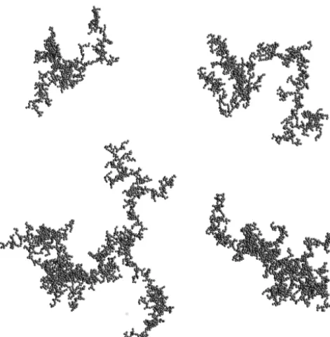
1. Pure, externally mixed black carbon particles are as-sumed to have a fractal aggregate morphology as shown in Fig. 1. The fractal morphology can be described by the statistical scaling lawNs=k0(Rg/a)Df, where Ns denotes the number of spherical monomers in the aggregate, Df and k0 are the fractal dimension and fractal prefactor, a is the monomer radius, and Rg=
q PNs
Figure 1. Examples of fractal aggregate model particles for com-puting optical properties of externally mixed black carbon. The ag-gregates consist of 1000, 1500, 2000, and 2744 monomers (in clock-wise order, starting from upper left).
mass-absorption cross sections at 550 nm wavelength that lie closer to experimental data, as was shown in Kahnert and Devasthale (2011). The monomer ra-dius can vary within a range of 10–25 nm (Bond and Bergstrom, 2006). Here it is assumed to bea=25 nm. This is consistent with field observations (Adachi and Buseck, 2008); also, it was shown (Kahnert, 2010b) that this choice of monomer radius in light scattering com-putations yields results for the single-scattering albedo of black carbon aggregates consistent with observations (Bond and Bergstrom, 2006).
The calculations in Kahnert and Devasthale (2011) were limited to aggregates up to Ns=600. In or-der to cover the size range of externally mixed black carbon in SALSA we had to extend these calcula-tions to aggregate sizes up toNs=2744, which corre-sponds to a volume-equivalent radius ofRV=350 nm (compare with Table 2). We used the multiple-sphere T-matrix code (Mackowski and Mishchenko, 2011), which is based on the numerically exact superposition T-matrix method for solving Maxwell’s equations. Fig-ure 2 shows some of the computed black carbon optical properties as a function of volume-equivalent particle radius and wavelength. All optical properties are aver-aged over particle orientations, where the orientation-averaging is performed analytically (Khlebstov, 1992). The absorption cross sectionCabsshows the characteris-tic decline at long wavelengths, where the refractive
in-dex of black carbon is changing only slowly (Chang and Charalampopoulos, 1990). Also, Cabs increases with particle size. For small particle sizes this increase goes as ∼RV3, which is typical for the Rayleigh scattering regime (Mishchenko et al., 2002).
2. Black carbon particles that are internally mixed with other aerosol components are morphologically very complex. It is technically beyond the reach of our present capabilities to build an aerosol-optics database with the use of morphologically realistic model parti-cles. However, it is possible to employ realistic model particles in reference computations for some selected cases. This has recently been done in different stud-ies (Kahnert et al., 2013; Scarnato et al., 2013, 2015). In the study by Kahnert et al. (2013), optical proper-ties of encapsulated aggregate model particles, such as the one shown in Fig. 3 (left), were computed in the range of 100–500 nm (volume-equivalent radius), for different black carbon volume fractions, and for wave-lengths from the UV-C to the mid-IR. The morpho-logical parameters characterizing these model particles were based on field observations (Adachi and Buseck, 2008); the coating material was sulfate. The computa-tions were performed with the discrete dipole approxi-mation (Yurkin and Hoekstra, 2007).
Figure 2. Absorption cross sectionCabs(upper left), single-scattering albedo SSA (upper right), asymmetry parameterg(bottom left), and backscattering cross sectionCbak(bottom right) of black carbon aggregates as a function of volume-equivalent radiusRVand wavelengthλ.
effect is neglected in the external-mixture model, result-ing in an underestimation ofCabs.
Note that in earlier studies (e.g. Jacobson, 2000) it was often tacitly assumed that a core-shell model would give the most accurate estimates of the aerosol optical prop-erties, owing to its morphological similarity to encap-sulated black carbon particles. However, the results in Kahnert et al. (2013) have clearly shown the shortcom-ings of the conventional core-shell model. But once we understand which morphological properties are most es-sential, and which ones make a minor contribution to the optical properties, we can devise model particles that account for the most important morphological effects, yet are sufficiently simple for computing a look-up ta-ble for large-scale modelling. It was proposed in Kah-nert et al. (2013) to use a core-shell model (hence ac-counting for the coating effect) in which only part of the carbon mass is contained in the core, and the remaining part is homogeneously mixed with the shell. The model particle is illustrated in Fig. 3 (right). The fractionfcof the carbon mass located in the core is a free parameter, with which one can interpolate between the two extreme models of the homogeneous mixture (fc=0, all carbon mass mixed with the shell) and the regular core-shell model (fc=1, all carbon mass in the core). This model has been referred to as the concentric core-grey-shell (CGS) model. The tuning of the free parameterfcin the model was done to fit the reference model of encapsu-lated aggregates as described in Kahnert et al. (2013). It was found thatfcis independent of particle size, black
carbon volume fraction, and of the optical property one wants to fit. However,fcdoes depend on the wavelength of light.
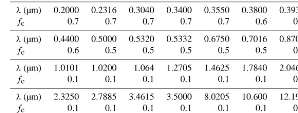
The CGS model has been employed in generating the new MATCH-optics look-up table. The shell material can be any mixture of water-soluble components. We use the same values offcas those determined in Kahn-ert et al. (2013). Its dependence on wavelength is given in Table 3.
3. In the mass transport model, we assume that all SIA components and all sea salt are internally mixed. We furthermore assume that in size bins 1–4, 0, 70, 70, and 100 %, respectively, of the black carbon, 0, 70, 70, and 70 % of the organic carbon, and 0, 1.3, 1.3, and 1.3 % of the dust are internally mixed; the remaining BC, OC, and dust mass is externally mixed. In SALSA, the mix-ing state depends on the size bin (see Table 2), and the mixing proportions are provided by the model results. In both the mass transport model and in MATCH-SALSA, the contribution to the effective refractive index of dust and black carbon is computed by the Maxwell Garnett EMT (Maxwell Garnett, 1904), while for all other com-ponents we use the Bruggemann EMT (Bruggemann, 1935).
Table 3. Core fractionfcin the core-grey-shell model as a function of wavelengthλ.
λ(µm) 0.2000 0.2316 0.3040 0.3400 0.3550 0.3800 0.3932
fc 0.7 0.7 0.7 0.7 0.7 0.6 0.6 λ(µm) 0.4400 0.5000 0.5320 0.5332 0.6750 0.7016 0.8700
fc 0.6 0.5 0.5 0.5 0.5 0.5 0.2
λ(µm) 1.0101 1.0200 1.064 1.2705 1.4625 1.7840 2.0460
fc 0.1 0.1 0.1 0.1 0.1 0.1 0.1 λ(µm) 2.3250 2.7885 3.4615 3.5000 8.0205 10.600 12.195
fc 0.1 0.1 0.1 0.1 0.1 0.1 0.1
Figure 3. Morphologically realistic encapsulated aggregate model for internally mixed black carbon (left), and core-grey-shell model (right).
The look-up tables contain results for Cext,Csca, g, and Cbakin 28 wavelength bands from the UV-C to the mid-IR. Computations with the CGS model were performed for 37 discrete BC volume fractions, namely,fBC=0.00, 0.01, . . . , 0.20, 0.25, . . . , 1.00. For the shell material, as well as for non-carbon containing particles, the table contains (depend-ing on the wavelength band) up to 40 discrete values of the real part and up to 18 discrete values of the imaginary part of the refractive index. The range of the refractive indices varies with wavelength; it is determined by those chemical compo-nents that, at each given wavelength, have the most extreme values of the refractive index. The optical properties are pre-averaged over particle sizes for each size bin. Thus we gen-erated one look-up table each for the mass transport model with its four size bins, and for SALSA with its 20 size bins. In SALSA it is assumed that the number density is constant in each size bin.
The MATCH-optics model computes in each grid cell and for each size bin the effective refractive index of the inter-nally mixed material by use of EMT. The corresponding opti-cal properties are obtained by linearly interpolating the clos-est pre-computed results in the look-up table. Size-averaging is performed by weighing the optical cross sections as well as g·Cscain each size bin with the number density per bin and adding over all bins. The integrated quantities are then divided by the total particle number density; the integral over
g·Cscais also divided by the size-averaged scattering cross section.
2.4 Methodology for comparing the optics models The new internal-mixture optics model with its BC fractal ag-gregate and core-grey-shell model particles accounts for sig-nificant morphological details in aerosol particles. The main question we want to address is whether or not this high level of detail is really necessary, i.e. whether it has any signifi-cant impact on optical properties modelled with a CTM. By significant we mean an impact that is comparable to other effects whose importance is well understood. Thus to make such an assessment we need to pick a well-understood ef-fect that can serve as a gauge, i.e. to which we can com-pare the impact of particle morphology on optical properties. We take the effect of aerosol microphysics as a gauge. As aerosol microphysics is well known to have a substantial im-pact on aerosol concentrations and size distributions (Ander-sson et al., 2015; Matsui et al., 2013), this effect will pro-vide us with a reference to which we can compare the impact of the morphological assumptions made in the aerosol-optics model. Thus we compute aerosol optical properties
1. with the MATCH mass-transport model (i.e. with aerosol microphysics switched off), in conjunction with the old optics model (abbreviated by MT-EXT, “mass-transport external mixture”);
2. with the MATCH mass-transport model in conjunction with the new optics model (MT-CGS, “mass-transport core-grey-shell”);
3. with the MATCH-SALSA model (i.e. with aerosol microphysics switched on), in conjunction with the old optics model (abbreviated SALSA-EXT, “MATCH-SALSA external mixture”); and
4. with the MATCH-SALSA model, in conjunction with the new optics model (SALSA-CGS, “MATCH-SALSA core-grey-shell”).
specifically, comparison of model set-ups EXT with MT-CGS, or SALSA-EXT with SALSA-CGS allows us to as-sess the impact of the morphological assumptions in the op-tics model. Comparison of MT-EXT with SALSA-EXT, or MT-CGS with SALSA-CGS will give us an estimate of how much the inclusion or omission of microphysical processes impacts modelling results of aerosol radiometric properties.
While statistical analyses can uncover general trends, it is difficult to understand the underlying physical reasons for model differences from an analysis of temporally and geo-graphically averaged model results. Therefore, we also con-sider a few case studies in some more detail. We take the optical properties modelled with different MATCH versions as input to a radiative transfer model and analyse the to-tal aerosol radiative forcing and the black carbon radiative forcing. The main goal is to understand how differences in single-scattering optical properties between the two optics models impact the outcome of the radiative transfer simu-lations. To keep the case studies within manageable bounds, we restrict ourselves to four geographic locations (two over land, two over the ocean), two instances (one represent-ing low-BC summer concentrations, one representrepresent-ing high-BC winter conditions), and we limit ourselves to compar-ing model set-ups MT-EXT, MT-CGS, and SALSA-CGS. More specifically, we consider one site over northern Italy (45.0◦N, 8.5◦E), one over the Mediterranean Sea (37.5◦N, 5.5◦E), one over Poland (52.6◦N, 21.0◦E), and one over the North Sea (52.0◦N, 2.7◦E). For the two instances, we pick 22 June 2007 12:00 UTC and 22 December 2007 12:00 UTC. Radiative transfer calculations are performed for each of these four sites and for both instances. Vertical profiles of the aerosol optical depth per layer, the single-scattering albedo, and the asymmetry parameter are used as input to the libRad-tran radiative libRad-transfer package (Kylling et al., 1998), assum-ing a plane-parallel atmosphere. For the surface albedo of the ocean we assume a spectrally constant value of 0.065, while for the spectrally varying surface albedo of the two land lo-cations we used MODIS observations for each of the two instances. The results were spectrally integrated to obtain the broadband radiative fluxes. The radiative transfer simulations were repeated for corresponding profiles of optical proper-ties (with a 1 km resolution) in the absence of black carbon, as well as for clear sky conditions. This allows us to compute differences in broadband radiative fluxes, i.e. the radiative effect of black carbon, and the radiative effect of all aerosol components. The results of this radiative transfer study are discussed in Sect. 3.2.
To further investigate the significance of the optics model for radiometric properties, we also look at optical properties relevant for remote sensing, namely, backscattering coeffi-cient and Ångström exponent. These results are discussed in Sects. 3.3 and 3.4, respectively.
3 Results
3.1 Aerosol optical properties in MATCH
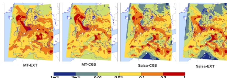
Figure 4 gives us a first impression of the differences be-tween the four model configurations. The extinction AOD is shown for MT-EXT (first from the left), MT-GCS (sec-ond), SALSA-CGS (third), and SALSA-EXT (fourth). The overall spatial patterns are similar. This is expected, since all model configurations used the same EMEP emissions and HIRLAM meteorological data. However, the magnitude of the AOD results can differ significantly among the four model runs (note the semi-logarithmic scale!). It is also re-markable that the differences between the two optics mod-els depend on whether we make this comparison within the mass-transport model (compare MT-EXT to MT-CGS), or within SALSA (compare SALSA-CGS and SALSA-EXT). It can also vary geographically. This merely confirms the complexity of aerosol-optics modelling. Replacing one tics model by another will not simply offset the resulting op-tical properties by some common factor; it will introduce a significant change in modelled optical properties, of which the magnitude and even the sign can be dependent on lo-cal conditions, such as the size distribution and the chemilo-cal composition of the aerosol particles.
This is also evident from a comparative analysis of geographically and temporally averaged aerosol optical properties. Table 4 shows aerosol optical depth (AOD), backscattering coefficient (BSCA), single scattering albedo (SSA), and asymmetry parameter (g), each at three dif-ferent wavelengths (355, 532, and 1064 nm), and each av-eraged over the whole model domain and over 1 month (December 2007). The columns show relative differences: for instance, MT(EXT,CGS)=(MT-EXT− MT-CGS)/(MT-CGS) is the relative difference of MT-model results obtained with the EXT and CGS optics models.
Comparison of the columns “MT(EXT,CGS)” and “SALSA(EXT,CGS)” illustrates the differences between the optics models in the absence and presence of aerosol-microphysical processes. As we already suspected from in-spection of Fig. 4, differences in the optics models defy sim-plistic explanations; both the magnitude and sign of these difference can be strongly dependent on the size-dependent chemical composition and mixing state of the aerosols, hence on the model version with which the optics models are be-ing compared. In our case, we see that compared to the CGS model, the EXT-optics model predicts higher values of AOD, BSCA, andgin the MT model, and lower values of SSA. In SALSA the roles of the CGS and EXT model are reversed.
Figure 4. Aerosol optical depth over Europe on 22 December 2007, 12:00 UTC (noon). Results are shown for the mass transport model in conjunction with the old external-mixture optics model (first to the left), and with the new internal-mixture/core-grey-shell/fractal BC aggregate model (second to the left), as well as for the MATCH-SALSA model in conjunction with the new optics model (third to the left) and old optics model (fourth to the left). The circles indicate the four locations used for radiative transfer studies. Note the semi-logarithmic colour scale!
Table 4. Averaged relative difference in aerosol optical depth (AOD), backscattering coefficient (BSCA), single scattering albedo (SSA) and asymmetry parameter (g), among the different model set-ups for December 2007. The average has been performed over a whole month and over all grid cells (horizontally for AOD, horizontally and vertically for all other optical properties). Each number corresponds to a relative difference between two model set-ups. For instance, MT(EXT,CGS)=(MT-EXT−MT-CGS)/(MT-CGS) compares results obtained with the mass transport model (MT) by using the two different optics models (EXT and CGS).
Xλ(nm) MT(EXT,CGS) SALSA(EXT,CGS) CGS(MT,SALSA) EXT(MT,SALSA)
AOD355 0.16 −0.28 −0.50 −0.19
AOD532 0.08 −0.14 0.00 0.25
AOD1064 0.18 −0.03 0.14 0.37
BSCA355 0.44 −0.01 −0.47 −0.23
BSCA532 0.26 −0.08 −0.19 0.11
BSCA1064 0.99 −0.01 −0.36 0.28
SSA355 −0.02 0.04 0.03 −0.03
SSA532 −0.02 0.05 0.04 −0.02
SSA1064 −0.07 0.08 0.08 −0.07
g355 0.06 −0.01 −0.10 −0.03
g532 0.10 −0.00 −0.06 0.04
g1064 0.17 −0.02 −0.11 0.06
been performed with the EXT model. If we compare the magnitudes of the entries in columns “MT(EXT,CGS)” and “SALSA(EXT,CGS)” with the corresponding magni-tudes of the entries in columns “CGS(MT,SALSA)” and “EXT(MT,SALSA)”, then we see that the differences be-tween the two optics models (EXT,CGS) are roughly of the same order as the differences between the two aerosol models (MT,SALSA). Thus, the main observation is that the choice of aerosol-optics model can have an effect on modelled opti-cal properties that is of comparable magnitude to the level of detail in the description of aerosol-microphysical processes.
While spatio-temporally averaged model results allow us to draw some general conclusions, it is difficult to understand the reasons for the observed differences from such an analy-sis. We will, therefore, complement this investigation in the
following sections with a more detailed analysis of some se-lected case studies.
3.2 Optical properties and radiative forcing
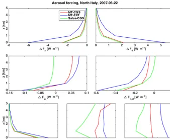
Figure 5. Aerosol forcing and optical properties at 532(CGS)/500(EXT) nm over northern Italy in June. Results are shown for the three model versions MT-EXT (blue), MT-CGS (red), and SALSA-CGS (green). The aerosol forcing is derived by taking the difference in radiative fluxes between an aerosol-laden and clear sky. The difference in direct (1Fs) and diffuse (1Fd) downwelling, as well as the diffuse upwelling (1Fu) and the net radiative flux (aerosol forcing) (1Fnet=1Fs+1Fd−1Fu), are shown in the first four figures (first and second row of plots). The optical properties aerosol optical depth (AOD), single scattering albedo (SSA), and asymmetry parameter (g) are shown in the third row of plots.
to investigate the impact of the optics model (CGS versus EXT).
The result for the optical properties obtained with the three model versions (AOD per layer, SSA, and g) at the wavelength 532(CGS)/500(EXT) nm, together with the ra-diative forcing for all aerosol components and black car-bon, respectively, can be seen in Figs. 5–10 for northern Italy and the Mediterranean on 22 June 2007. Each figure shows the differences in direct solar flux1Fs(top left), dif-fuse downwelling flux 1Fd (top right), diffuse upwelling flux1Fu(centre left), and net radiative flux1Fnet=1Fs+ 1Fd−1Fu (centre right), where either the difference be-tween aerosol-laden and clear sky conditions is considered (Figs. 5 and 6), or the difference between fluxes in the pres-ence and abspres-ence of black carbon (Figs. 9 and 10). Here, downwelling fluxes are obtained by integrating the radi-ance over all azimuthal angles, and over polar angles from 90 to 180◦, where the positivez axis is directed from the ground to the top-of-atmosphere (TOA). Similarly, the up-welling flux is obtained by integrating the radiance over all azimuthal angles, and over polar angles from 0 to 90◦. TOA results for the other geographical locations are sum-marized in Table 5 in terms of aerosol forcing (1Fnet=
Fnet(with aerosol particles)−Fnet(no aerosol particles)), and in Table 6 in terms of black carbon forcing (1Fnet= Fnet(with black carbon)−Fnet(no black carbon)). The wave-lengths 532(CGS)/500(EXT) nm are near the maximum of the solar spectrum. Each figure has a vertical span of 5 km, which comprises that part of the troposphere where most aerosol particles are concentrated in the cases we picked. 3.2.1 Comparison of aerosol microphysics and
mass-transport model
Figure 6. Same as Fig. 5 but over the Mediterranean.
extinction in the form of scattering results in the generation of diffuse flux; the downwelling diffuse flux accumulates downward, resulting in an increasing excess of downwelling flux1Fdin the presence of aerosol components as one ap-proaches the surface. The upwelling fluxFuis generated by scattering in the atmosphere and reflection at the surface. Since aerosol extinction reduces the net radiative flux as one approaches the surface, less upwelling diffuse flux is gener-ated at low altitudes; hence, the difference in upwelling flux 1Fu between an aerosol-laden and a clear sky atmosphere is negative near the surface. However, it increases with al-titude, because at higher altitudes the magnitude of the dif-ference (aerosol–clear sky) in the net radiative flux that can be converted into upwelling diffuse flux decreases at higher altitudes.
If we focus now on differences in the radiative net flux 1Fnet at high altitudes, i.e. the radiative forcing effect of aerosol particles, then we see significant differences between the mass transport model (MT, red) and SALSA (green) at both geographic locations. It is evident that the main causes of these are corresponding differences in the diffuse up-welling flux1Fu.
At both locations the diffuse upwelling flux is smaller for SALSA then for MT, but for different reasons. Over the Mediterranean (Fig. 6), the AOD is significantly smaller for SALSA than for MT, resulting in less extinction of the di-rect flux, hence less generation of diffuse flux, and a smaller radiative cooling effect for SALSA.
Over northern Italy (Fig. 5), there is almost no difference in AOD between the two models. It can be seen from the AOD profile that the majority of aerosol particles reside in the lowest 1 km near the surface. However, above 1 km the re-sults of1Fuobtained with SALSA and MT diverge with in-creasing altitude. This is a result of the reflection by the near-surface aerosol layer, which is different in the two models. In MT the SSA is higher than in SALSA, resulting in more scattering, and thus in more diffuse radiation. The asymme-try parameter is larger in MT than in SALSA; correspond-ingly, the partitioning in MT between downwelling and up-welling radiation is somewhat shifted in favour of the for-mer. However, this only partially counteracts the generation of a higher amount of diffuse upwelling radiation in MT due to the higher SSA. The net effect is a higher value of1Fu in MT, and hence a larger radiative cooling effect at higher altitudes.
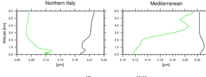
To further analyse the difference in optical properties be-tween MT and SALSA, we look at the aerosol masses and the relative sizes of the particles. Figure 7 shows vertical pro-files of the effective radiusreff defined according to Eq. (1), in SALSA (green), and the MT model (black) over northern Italy (left) and over the Mediterranean (right).
reff=
R∞
0 n(r)π r 2·rdr
R∞
0 n(r)·π r2dr
ni-Figure 7. Effective radius,reff, for the two chemical transport model versions MT and SALSA over northern Italy and the Mediterranean on 22 June 2007 at 12:00.
trate (fourth row) for both northern Italy (first column) and the Mediterranean (second column). We focus on the total aerosol mass, which is expected to impact the aerosol optical depth. The aerosol optical depth is dependent on the number density (which, in turn, increases with the mass mixing ratio), as well as on the extinction cross section (which generally in-creases with the effective radius of the particles). Over north-ern Italy, the SALSA model predicts a larger mass mixing ra-tio than the MT model (Fig. 8, upper left) and a smaller par-ticle size (Fig. 7, left). This results in a higher number den-sity but a smaller extinction cross section. These two effects cancel almost exactly, resulting in nearly identical aerosol optical depths predicted with the two models (Fig. 5, bot-tom left). By contrast, over the Mediterranean, the two mod-els predict similar mass mixing ratios (Fig. 8, upper right), while SALSA predicts a much lower effective radius than the MT model (Fig. 7, right). As a consequence, the optical depth is significantly lower in SALSA than in MT (Fig. 6, bottom left). The SSA is lower in SALSA than in MT. This is mainly caused by the fact that the effective radius is smaller in SALSA than in MT, since SSA is usually increasing with size.
For the other two geographical locations and the second time event, the TOA results are summarized in Table 5. Over the North Sea, northern Italy, and the Mediterranean, the TOA forcing is strongest in the MT-EXT model (mass trans-port with old optics model), it is smaller in the MT-CGS model (mass transport with new optics model), and weak-est in the SALSA-CGS model (aerosol-microphysics with new optics model). However, over Poland the negative forc-ing in SALSA-CGS is strongest among the three models in the summer, and second strongest in the winter. This can be explained by SALSA having a larger amount of aerosol par-ticles throughout the column at that site, especially more sul-fate, which, when externally mixed, contributes to a larger amount of scattering and therefore a higher SSA and a larger diffuse upwelling radiative flux.
We now compare radiative fluxes in the presence and ab-sence of black carbon, which we refer to as the “black carbon
radiative effect”. Figures 9 and 10 show the radiative effect of black carbon together with the optical properties with and without black carbon. Again, differences in1Fnetat TOA are mainly caused by corresponding differences in the upwelling diffuse radiative flux1Fu. In these figures, we have to focus on the difference in the optical properties when analysing the radiative fluxes. The general pattern can be seen in Fig. 9, which shows the differences in radiative fluxes and in the op-tical properties over northern Italy. The direct solar flux (up-per left) decreases with decreasing altitude owing to extinc-tion. The magnitude of the decrease mainly reflects the dif-ferences in optical depth in the presence and absence of black carbon (bottom left), which is larger in SALSA than in MT. The decrease in solar flux does not automatically result in an increase in the downwelling diffuse flux with decreasing alti-tude (upper right), as it was in the comparison of fluxes in the presence and absence of all aerosol components. The situa-tion is more complex now. Near the surface, where the optical depth is largest, the difference in SSA in the presence and ab-sence of black carbon is large in the MT model (bottom cen-tre, red lines), and smaller in SALSA (green lines). As a re-sult, absorption contributes more to the total extinction in the MT model than in SALSA (at least near the surface). Hence, the portion of the downwelling flux that is absorbed on its way downward is larger in the MT model than in SALSA, resulting in a decrease of the diffuse downwelling flux with decreasing altitude (upper right, red line). The differences be-tween the two models in the diffuse upwelling flux are very small (centre left, red and green lines). This is the result of cancelling effects; for instance, there is less direct solar flux, but more diffuse downwelling flux in SALSA that can be converted into diffuse upwelling flux through scattering. As a result, the differences between both models in the net flux (centre right, red and green lines) are almost negligible.
Figure 8. Vertical distribution of aerosol particles in northern Italy and over the Mediterranean on 22 June 2007 at 12:00.
especially the SSA, differ in the presence and absence of BC by almost the same amount in both models.
Table 6 shows the black carbon forcing for all the four ge-ographical locations and both months. As a general trend, large differences in BC concentrations are visible as cor-responding differences in BC forcing. For instance, near-surface BC winter concentrations in northern Italy are about a factor of 10 higher than in summer; summer concentra-tions over the Mediterranean are more than a factor of 2 higher than in winter; in northern Italy in winter, SALSA predicts more than 2 times higher BC concentrations than the mass-transport model, while over the Mediterranean in win-ter the role of the two models is reversed (not shown). All of this corresponds to the respective BC-forcing rates in Ta-ble 6. However, when the differences in BC concentrations are small, then there is no clear relation between the con-centration differences and the corresponding differences in BC-forcing rates. For instance, as we see in Fig. 8, there is almost no difference between the BC concentrations
com-puted with the two models over the Mediterranean in sum-mer. But the table shows that the mass-transport model pre-dicts a slightly higher forcing rate than SALSA. A possible cause is the difference in the size distributions in SALSA and the mass-transport model.
3.2.2 Comparison of the two optics models
The comparison between SALSA and the MT model in the previous section served two purposes. First, it helped us to develop a basic understanding of the effects of aerosol parti-cles and black carbon on radiative fluxes. Second, it provided us with a gauge for assessing the importance of the aerosol-optics model, which will be the subject of this section.
Table 5. The aerosol forcing at the top of the atmosphere (TOA), 1Fnet,TOA(W m−2), for the four different geographical locations, one summer (22 June 2007, 12:00) and one winter (22 Decem-ber 2007, 12:00) event, and three model versions, EXT, MT-CGS, and SALSA-CGS.
MT-EXT MT-CGS SALSA-CGS
Summer Poland −0.21 −0.21 −0.77 North Sea −0.34 −0.29 −0.24 Northern Italy −0.06 −0.05 0.01 Mediterranean −1.20 −0.99 −0.30
Winter Poland −4.41 −2.00 −2.18 North Sea −2.85 −1.21 −0.86 Northern Italy −1.15 −0.53 −0.57 Mediterranean −0.09 −0.04 −0.03
Mediterranean. Again, the upwelling flux has the dominant impact on the behaviour of the TOA net radiative flux. Over northern Italy (Fig. 5) the diffuse upwelling flux is larger for the EXT model above 1 km, whereas it is smaller below 1 km and at the bottom of the atmosphere (BOA). The AOD pro-file reveals that in the EXT model extinction is stronger than in the CGS model throughout the tropospheric column. As a result, there is more diffuse downwelling flux being gener-ated in EXT than in CGS. At the bottom of the atmosphere (BOA) extinction of the direct flux is stronger than gener-ation of diffuse downwelling flux; hence, less downwelling flux is reflected by the surface, resulting in less BOA up-welling diffuse flux in EXT than in CGS. Higher up in the troposphere, the upwelling diffuse flux is mostly generated by atmospheric scattering rather than reflection from the sur-face. As the SSA in EXT is higher than in CGS, more diffuse flux is generated, resulting in a stronger radiative cooling ef-fect in EXT than in CGS.
Over the Mediterranean (Fig. 6), the EXT and CGS mod-els have almost identical AOD profiles in the green part of the spectrum. However, at longer wavelengths EXT predicts sub-stantially higher AOD values than CGS (see the Supplement provided with figures of the different optical properties and wavelengths). For instance, atλ=1020 nm the near-surface AOD per layer computed with the EXT model is about twice as high as that computed with the CGS model. This explains the larger amount of diffuse broadband radiation generated in the EXT model, which results in a stronger negative TOA net flux in EXT as compared to the CGS model. Note that the differences in SSA between EXT and CGS are less than 0.03, while the differences in g are as much as 0.07. The higher values ofgin EXT may contribute to the large amount of diffuse downwelling radiation in that model; however, the dominant effect is likely to be the high optical depth at red and IR wavelengths (Supplement).
Table 5 summarizes the TOA net radiative flux at all four geographical locations for both June and December. The largest differences among the models are seen in
Decem-Table 6. Same as Decem-Table 5 but for black carbon forcing.
MT-EXT MT-CGS SALSA-CGS Summer Poland 1.02×10⁻² 1.16×10⁻² 1.20×10⁻² North Sea 1.71×10⁻² 1.54×10⁻² 1.49×10⁻² Northern Italy 4.61×10⁻² 7.77×10⁻² 7.86×10⁻² Mediterranean 8.54×10⁻³ 6.45×10⁻³ 2.41×10⁻³ Winter Poland 4.03×10⁻² 3.56×10⁻² 6.83×10⁻² North Sea 1.95×10⁻² 2.28×10⁻² 4.97×10⁻³ Northern Italy 6.73×10⁻² 1.08×10⁻¹ 1.46×10⁻¹ Mediterranean 6.03×10⁻⁴ 1.34×10⁻³ 3.13×10⁻⁴
ber at the two northernmost locations, i.e. Poland and the North Sea. At these two places, the total aerosol amount (not shown) is significantly higher than at the other two locations farther south, giving rise to larger absolute changes in the aerosol forcing.
The black carbon forcing in Figs. 9 (northern Italy) and 10 (Mediterranean) display different behaviours in radiative fluxes, comparing the EXT (blue) and CGS (red) model re-sults. Over northern Italy, the net black carbon forcing is more significant than over the Mediterranean in Fig. 10 due to higher levels of BC; see Fig. 8. As can be seen in Fig. 9, the differences in optical properties computed with and with-out black carbon are larger in the CGS model than in the EXT model, particularly for the SSA. This means that in the CGS model the presence of black carbon causes more ab-sorption than in the EXT model, thus generating less diffuse downwelling and upwelling flux by scattering. As a result, the CGS model predicts more radiative warming, i.e. a higher TOA radiative net flux than the EXT model. The reason for this is that (i) the CGS model treats externally mixed soot as aggregates, which have a lower SSA than the massive black carbon spheres in the EXT model; and (ii) the CGS model treats internally mixed soot as a coated core-grey-shell model, which accounts for focusing of electromagnetic radi-ation onto the carbon core, thus enhancing absorption, i.e. lowering the SSA, while the EXT model treats all black car-bon as externally mixed.
op-Figure 9. Black carbon forcing and optical properties at 532(CGS)/500(EXT) nm over northern Italy in June. Results are shown for the three model versions MT-EXT (blue), MT-CGS (red), and SALSA-CGS (green). The black carbon forcing is derived by taking the difference in radiative fluxes between an aerosol-laden sky including black carbon and an aerosol-laden sky omitting black carbon. The difference in direct (1Fs) and diffuse (1Fd) downwelling, as well as the diffuse upwelling (1Fu) and the net radiative flux (aerosol forcing) (1Fnet= 1Fs+1Fd−1Fu), are shown in the first four figures (first and second row of plots). The optical properties aerosol optical depth (AOD), single scattering albedo (SSA), and asymmetry parameter (g) are shown in the third row of plots.
tics model has a stronger effect than the inclusion of aerosol microphysics (e.g. Fig. 9), while in other cases it is the other way round (e.g. Fig. 6). We can also inspect Tables 5 and 6 and arrive at the same result.
In the following two subsections, we will focus on the se-lected case studies and discuss the significance of the optics model for radiometric quantities that are relevant for remote sensing applications.
3.3 Backscattering coefficient
From ground-based and space-borne lidar measurements one can obtain the aerosol backscattering coefficientβ, which is proportional to the backscattering cross section Cbak of the particles and the aerosol number density. Figure 11 shows vertical profiles ofβ computed at two locations and at two instances, as indicated in the figure headings. Each panel shows computational results obtained with the three differ-ent model versions. The figure shows results for the second Nd:YAG harmonic of 532 nm. Corresponding results com-puted for wavelengths of 355 and 1064 nm lead to similar conclusions.
We saw in Fig. 8 for June over northern Italy (upper left) that SALSA predicts an aerosol mass mixing ratio, and hence a particle number density that is higher than that in the MT model. But we also saw in Fig. 7 (left) that SALSA predicts lower values of reff. This results in lower values of Cbak. We see in Fig. 11 (upper left) that the effect on β of the higher number density dominates over the effect of the lower reff, resulting in values ofβ that are about 30 % higher in SALSA (green line) than in the MT model (red line). Over the Mediterranean, both SALSA and the MT model predict similar mass mixing ratios (Fig. 8, upper right), but SALSA still predicts substantially lower values ofreff(Fig. 7, right). The result is thatβ computed with the MT model (red line) is almost twice as high as the corresponding results obtained with SALSA (green line) (Fig. 11, upper right).
un-Figure 10. Same as Fig. 9 but over the Mediterranean.
Figure 11. Backscattering coefficient at a wavelength of 532 nm in northern Italy and the Mediterranean and at two different time events (22/6 and 22/12/2007 at 12.00), computed with the three model versions: MT-EXT (blue), MT-CGS (red), and SALSA-CGS (green).
derestimated retrieval results for the particle number density.) The differences between the two optics models are on the same order of magnitude (and often even larger) than the corresponding differences between the SALSA and the MT versions of the aerosol transport model.
3.4 Ångström exponent
The Ångström exponentαin a wavelength interval [λ1,λ2] is defined as
α= −log(τ (λ1)/τ (λ2))
log(λ1/λ2)
, (2)
Table 7. Ångström exponent in the wavelength region 532– 1064 nm for the four different geographical locations, one summer (22 June 2007, 12:00) and one winter (22 December 2007, 12:00) event, and three model versions, MT-EXT, MT-CGS, and SALSA-CGS.
MT-EXT MT-CGS SALSA-CGS Summer Poland 0.32×100 0.12×101 0.28×101 North Sea 0.80×100 0.12×101 0.21×101 Northern Italy 0.11×101 0.11×101 0.15×101 Mediterranean 0.36×100 0.12×101 0.21×101 Winter Poland 0.80×100 0.12×101 0.22×101 North Sea 0.79×100 0.11×101 0.14×101 Northern Italy 0.13×101 0.10×101 0.12×101 Mediterranean 0.13×101 0.98×100 0.14×101
computing α are unpredictable, even the sign of the error. When used in a size retrieval algorithm the retrieval errors caused by the EXT model would be equally hard to pre-dict. The difference between the MT and SALSA model is larger, but not much larger, than the differences between the old and new optics models. Note that the performance of the MT model could be improved in comparison to SALSA by modifying the assumed size distribution in the MT model. By contrast, the differences between the two optics models are rather fundamental; they are caused by the simple treatment of aerosol morphology in the EXT model.
4 Conclusions
We have implemented a new aerosol-optics model in a re-gional chemical transport model. The new model differs from an earlier optics model described in Kahnert (2008) in three essential points. (i) While the old model treats all chemical components as externally mixed, the new model accommo-dates both external and internal mixtures of aerosol species. (ii) The old model treats black carbon particles as homoge-neous spheres; the new model assumes a fractal aggregate morphology with fractal parameters based on observations. Mass absorption cross sections and single scattering albedos computed with this model have previously been evaluated by comparison with measurements (Kahnert, 2010b). (iii) The new model describes internally mixed black carbon particles by a recently developed “core-grey-shell” model (Kahnert et al., 2013). This model accounts for the inhomogeneous in-ternal mixing state of black carbon aggregates encapsulated in a shell of liquid-phase material. The model has been eval-uated by comparison with reference computations based on observation-derived realistic models for encapsulated fractal aggregates (Kahnert et al., 2013). Item (i) has been incorpo-rated in other CTMs earlier (e.g. Saide et al., 2013); however, to the best of our knowledge, items (ii) and (iii) go signif-icantly beyond the current state-of-the-art of aerosol-optics models employed in CTMs. The main question of the present
study is whether or not such a substantial level of detail in the description of aerosol morphology and optical properties is needed in a CTM.
We first performed a comparison of optical properties av-eraged over the entire model domain and over 1 month. To gauge the differences between the new and old optics models, we furthermore compare two model versions of the CTM with different levels of detail in the aerosol pro-cess descriptions, namely, one version that includes aerosol-dynamic processes, and a simpler mass-transport model, in which aerosol microphysics is switched off. The importance of aerosol microphysics is well understood and can there-fore serve as a reference. We found that the differences in optical properties between the two optics models are of the same order as those between the versions that include and ex-clude microphysical processes. For example, the aerosol op-tical depth computed with the two optics models differs by
−28 to 18 %; differences obtained by inclusion or omission of aerosol microphysics are between−50 and 37 %. Corre-sponding differences in the backscattering coefficient are−8 to 99 % and−47 to 28 %, respectively. Analogous observa-tions can be made for other radiometric properties.
We furthermore wanted to understand how the differences in optical properties impact radiative transfer processes in an aerosol-laden atmosphere. To this end we compare ra-diative fluxes modelled with the old and new optics mod-els. The comparison showed that the differences in radia-tive net fluxes between the two optics models are of similar magnitude as corresponding differences between the aerosol-microphysics and mass-transport models.
These results strongly suggest that simplifications in the assumptions on aerosol morphology in the optics model can introduce substantial errors in modelled radiative fluxes and observables relevant to remote sensing. In chemistry-climate models such errors would enter into the simulation of the direct aerosol radiative forcing effect and add to all other sources of error in the model. In model evaluations that make use of remote sensing observations these errors would com-plicate the comparison between model results and observa-tions.
The modifications to the morphology assumptions in the optics model were limited to black carbon particles. There are many other aerosol particles with complex morphologi-cal properties, such as mineral dust, which our optics model still treats by a simple homogeneous-sphere model. The find-ings of our study should be an incentive for improving the description of dust and volcanic-ash optical modelling in CTMs. A recent review of our current state of knowledge on aerosol morphology and aerosol optics for a variety of differ-ent aerosol particles can be found in Kahnert et al. (2014).
just our aerosol-optics model, possibly coupled to a radiative transfer model. Many data-assimilation methodologies, such as the variational method, require a linear (or, at least, lin-earized) observation operator. In the old optics model, which assumes externally mixed aerosol particles, the observation operator is, indeed, linear (Kahnert, 2008). This largely ex-plains why external-mixture optics models are widely used in chemical data assimilation systems (e.g. Kahnert, 2008; Benedetti et al., 2009; Liu et al., 2011). However, the new optics model we introduced here does not provide us with a linear map from the aerosol concentrations to the optical parameters. To what extent one could linearize this model and make use of its Jacobian in a data assimilation system mainly depends on the degree of nonlinearity, which would need to be investigated thoroughly.
Code availability
Appendix A: Size-averaged optical properties in the external-mixture optics model
The external-mixture optics model is based on using four size bins that cover the dry-radius intervals[rmin, rmax] = [0.01, 0.05], [0.05, 0.5], [0.5, 1.25], and [1.25, 5] µm. The geomet-ric mean radiusR=
√
rminrmax=0.5(logrmin+logrmax)is given in each of these intervals by R1=0.022 µm, R2= 0.158 µm,R3=0.791 µm, andR4=2.5 µm. In each size bin it is assumed that the particle number density is given by a log-normal distribution
ni(r)=Ni0/( √
2π rlnσi)exp[−ln2(r/Ri)/(2ln2σi)], (A1) whereσ1=σ3=σ4=1.8,σ2=1.5 are based on measure-ments in Neusüß et al. (2002). Here,Ni0would be the total number density per mode if each size mode extended from r=0 to r= ∞. However, since each mode is truncated at the bin boundariesrminandrmax, the number densityNi of particles per size bin is obtained from integration over this finite interval, i.e.
Ni= rimax
Z
rimin
ni(r)dr=Ni0 1 2
h
erf(ximax)−erf(ximin)i, (A2)
where ximax=ln(rimax/Ri)/( √
2 lnσi), and similarly for ximin. Analogously, one obtains the particle-mass densityMi in each size bin by integrating over the truncated log-normal mode, which yields
Mi= 4 3π ρi
rimax
Z
rimin
ni(r)r3dr (A3)
=4
3π R 3
iρiNi0exp
9 2ln 2σ i 1 2 h
erf(yimax)−erf(yimin)
i
,
whereyimax=ximax−3 lnσi/ √
2, and similarly forymini , and whereρi is the density of the aerosol particles in theith size bin. From this we obtain the desired relation for converting the mass densityMiinto the number densityNi:
Ni= Mi 4 3π R
3 iρi
· erf(x
max
i )−erf(ximin) exp92ln2σi
erf(yimax)−erf(ymini ) . (A4)
Mass-mixing ratiosXi are simply converted into mass den-sities Mi according to Mi=Xiρair, whereρair denotes the density of air.
In the external-mixture optics database, optical properties are pre-computed by integrating optical properties at discrete sizes over the truncated log-normal size distribution. This in-tegration is done numerically with a high size resolution. The computation is performed for different refractive indicesm,
optical wavelengthsλ, and for each size bini. Thus, one ob-tains e.g. extinction cross sectionsCext(λ, m, i), which can be saved in a look-up table.
Secondary inorganic aerosols as well as organic aerosols and sea salt are assumed to be hydrophilic. We use the pa-rameterization by Gerber (1985) to compute the wet radius rw from the aerosol dry radiusR, from which we obtain the volume fraction of waterfw=(rw3−R3)/R3. The effective refractive indexmof the aerosol–water mixture is computed from that of the dry aerosol,ma, and of water,mwby use of effective-medium theory. In each grid cell, we obtain from the MATCH model, for each size biniand for each aerosol componentk, the number densityNi(k). From that we com-pute the ensemble-averaged extinction cross section
¯
Cext(λ)= 1 N X k 4 X
i=1
Ni(k)Cext(λ, m(k), i), (A5) where the total number density is given by
N=X
k 4
X
i=1
Ni(k). (A6)
Note that the ensemble-average involves an average over both size and chemical composition. The ensemble-averaged scattering cross section C¯sca(λ) is computed analogously. From this we obtain the averaged single-scattering albedo
¯
ω(λ)= ¯
Csca(λ) ¯
Cext(λ)
. (A7)
The phase functionp(2), and hence its first Legendre mo-ment, known as the asymmetry parameterg, are normalized quantities. Here2denotes the scattering angle. To average these quantities, one first needs to “de-normalize” by multi-plying them by the scattering cross section. Thus,
¯
p(2;λ)= 1
NC¯sca(λ)
X
k 4
X
i=1
Ni(k) (A8)
Csca(λ, m(k), i)p(2, m(k), i;λ),
¯
g(λ)= 1
NC¯sca(λ)
X
k 4
X
i=1
Ni(k) (A9)
Csca(λ, m(k), i)g(m(k), i;λ).
Once the ensemble-averaged optical properties in each grid cell of the model domain have been computed, one can compute radiometric observables, such as the extinction aerosol optical depth
τext(λ)=
X
z
N (z)C¯ext(λ, z)1z, (A10)
or the backscattering coefficient βbak(λ, z)=
1 4πN (z)
¯
Appendix B: Size-averaged optical properties in the internal-mixture model
In SALSA the number density as a function of particle ra-dius, n(r), is given by a step function with ni(r)=consti in each size bin i. This makes the pre-integration of opti-cal properties over each size bin rather simple. On the other hand, we no longer assume that all aerosol components are externally mixed. Thus the ensemble average over differ-ent chemical compondiffer-ents kis no longer given by a simple summation P
k· · ·, as it was in the external-mixture model. Rather, for each size bin in which several aerosol components are internally mixed one computes an effective refractive in-dex,meff, by use of effective-medium theory. One then reads the optical properties for that refractive index from the look-up table. Finally, one computes ensemble-averaged optical properties by summing over all size bins,P
i· · ·.
Appendix C: Effective-medium theory
In effective-medium theory (EMT) one considers a compos-ite material consisting of two materials with refractive in-dicesm1andm2and volume fractionsf1andf2=1−f1. One then invokes assumptions about the topology of the mix-ture and derives a formula for the effective refractive index, meff, of the composite material. For instance, it is often the case that f1f2. In this case one can regard the first ma-terial as a host matrix that contains inclusions of the sec-ond material. This is the basis of the Maxwell Garnett EMT (Maxwell Garnett, 1904). The resulting expression formeff is
meff=
s
m21m 2
1(2−2f2)+m 2
2(1+2f2) m21(2+f2)+m22(1−f2)
. (C1)
In the Bruggemann EMT (Bruggemann, 1935) one treats both materials more symmetrically; both components are as-sumed to be embedded in a host matrix with an effective re-fractive index given by
meff=
1
4m 2
1(2−3f2)+m22(3f2−1) (C2)
+
r
1 16
h
m21(2−3f2)+m22(3f2−1)
i2
+1
2m 2 1m22
!1/2
.
Although not immediately manifest, this equation is symmet-ric under exchange of the two materials.