Optimization of NWP model closure parameters using total energy norm of forecast error as a target

(1)

www.geosci-model-dev.net/7/1889/2014/ doi:10.5194/gmd-7-1889-2014

Optimization of NWP model closure parameters using total energy

norm of forecast error as a target

P. Ollinaho1,2, H. Järvinen2, P. Bauer3, M. Laine1, P. Bechtold3, J. Susiluoto1,2, and H. Haario4 1_{Finnish Meteorological Institute, Helsinki, Finland}

2_{University of Helsinki, Department of Physics, Helsinki, Finland} 3_{European Centre for Medium-Range Weather Forecasts, Reading, UK} 4_{Lappeenranta University of Technology, Lappeenranta, Finland}

Correspondence to: P. Ollinaho ([email protected])

Received: 6 November 2013 – Published in Geosci. Model Dev. Discuss.: 17 December 2013 Revised: 27 June 2014 – Accepted: 17 July 2014 – Published: 2 September 2014

Abstract. We explore the use of dry total energy norm in improving numerical weather prediction (NWP) model fore-cast skill. The Ensemble Prediction and Parameter Estima-tion System (EPPES) is utilized to estimate ECHAM5 at-mospheric GCM (global circulation models) closure param-eters related to clouds and precipitation. The target criterion in the optimization is the dry total energy norm of 3-day forecast error with respect to the ECMWF (European Cen-tre for Medium-Range Weather Forecasts) operational analy-ses. The results are summarized as follows: (i) forecast error growth in terms of energy norm is slower in the optimized than in the default model up to day 10 forecasts (and be-yond), (ii) headline forecast skill scores are improved in the training sample as well as in independent samples, (iii) the decrease of the forecast error energy norm at day three is mainly because of smaller kinetic energy error in the trop-ics, and (iv) this impact is spread into midlatitudes at longer ranges and appears as a smaller forecast error of potential en-ergy. The interpretation of these results is that the parameter optimization has reduced the model error so that the forecasts remain longer in the vicinity of the analyzed state.

1 Introduction

Tuning of closure parameters in atmospheric modeling is a recurring topic. In research, the aim is to improve physical realism of subgrid-scale physical processes and to maintain or improve the general model behavior, such as reproduction of observed variability. In operational applications, such as

numerical weather prediction (NWP), the aim is also to in-crease the predictive skill. Tuning procedures in modeling are predominantly manual and there are no generally applicable or accepted algorithmic tools in everyday use. One reason is that in multiscale and multiphase systems the model response to closure parameter variations is very nonlinear and general nonstationary inverse problem tools can fail. Therefore re-sults may be promising in idealized cases but this does not seem to carry on to more demanding real-world estimation cases. This difficulty is nicely illustrated in Schirber et al. (2013), where the inverse problem realism is gradually in-creased from a synthetic to fully realistic estimation in case of an atmospheric general circulation model. The parameter-augmented state filter works well in an idealized setup but is less successful in realistic estimation cases.

(2)

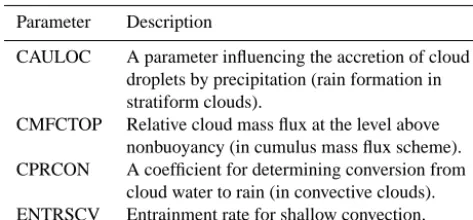
Table 1. ECHAM5 closure parameter subset used in model

opti-mization.

Parameter Description

CAULOC A parameter influencing the accretion of cloud droplets by precipitation (rain formation in stratiform clouds).

CMFCTOP Relative cloud mass flux at the level above nonbuoyancy (in cumulus mass flux scheme). CPRCON A coefficient for determining conversion from

cloud water to rain (in convective clouds). ENTRSCV Entrainment rate for shallow convection.

improvements in all model fields would assure a model-wide improvement, but the construction of correct weights for the all the variables would be impractical. However, a too simple target is not likely to lead to a univocally improved model. This paper presents atmospheric dry total energy norm as a target for model optimization. In recent years, various energy norms have appeared in NWP literature mainly in the context of seeking the fastest growing structures to be used as ini-tial state perturbations in ensemble prediction systems (e.g., Farrel, 1988; Palmer et al., 1994; Errico, 2000), as well as in forecast sensitivity studies (e.g., Gelaro et al., 1998; Orrell et al., 2001; Mitchell et al., 2002). Here we apply the dry total energy norm in the opposite sense of the former: we seek a model which tends to have the slowest possible forecast error growth in terms of dry total energy norm. As the energy norm is computed as an integral over the entire model atmosphere, it is not selective to any particular model variable, level, or geographical region. It is thus a potentially powerful target.

2 Experiment configuration

The ECHAM5.4 atmospheric general circulation model (Roeckner et al., 2003) is used here with a coarse hori-zontal resolution of T42 and 31 vertical layers, the model top being at 10 hPa. We consider the same four closure pa-rameters (Table 1) that were estimated in Ollinaho et al. (2013b), and studied in Järvinen et al. (2010). These influ-ence parametrized clouds and precipitation, and, even though considered here only from the NWP viewpoint, they are also of great interest when considering the model climatology.

A more complete description of the ensemble prediction system (EPS) emulator is given in detail in Ollinaho et al. (2013b). A concise overview is provided in the following: the operational ensemble of initial states produced by ECMWF EPS (ENS) has been used to generate initial uncertainties. A total of 50 perturbed initial states, as well as the con-trol state, are used for twice-daily (00:00 and 12:00 UTC – universal time coordinated) forecasts over a period of 3 months (January–March 2011). The initial-time parameter

variations, sampled via the EPPES algorithm, represent the model error.

The EPPES algorithm was introduced in Laine et al. (2012), who also demonstrated the algorithm use with a stochastic version of the Lorenz-95 model (Lorenz, 1996; Wilks, 2005). The EPPES algorithm approaches the prob-lem of estimating model parametersθby assuming it to be a realization from a background parameter uncertainty distri-bution that is approximated by a multivariate Gaussian dis-tribution, with a mean vectorµ(of dimensionp) and ap×p

covariance matrix6. For each time windowi, the optimal parameters,θ_i, are a sample from this distribution as

θi∼N (µ,6), i=1,2, . . . (1)

The estimation problem is thus shifted to estimating these unknown, but static in time, distribution parameters (or hy-perparameters). The mean of the distributionµcorresponds to parameter values that perform best on average considering all weather types, seasons, etc., and6 indicates how much these values vary between time windows due to inaccurate parametrization schemes and other modeling errors. Thus,6

provides objective information about uncertainties related to the estimated parameters.

The algorithm first draws a sample from an initial distri-bution, and these parameter values are used in an ensemble of forecasts. The likelihood of each forecast is then evalu-ated with respect to given criteria, and each parameter vector is weighted by the likelihood. A resample is drawn from the weighted parameter sample, favoring parameter values asso-ciated with high likelihood (known as importance sampling). Finally, the hyperparametersµ and6 are updated with the weighted sample. A new sample is then drawn for the next time window from the updated distribution. The algorithm steps can be written are as follows:

1. Initialize the hyperparameters µ₀ and60. The distri-bution N (µ₀,60) acts as the prior for θ for the first time window and as the proposal distribution for the first sample.

2. For each time instancei, draw a sample of proposed val-ues for the parametersθi – call themθ˜

j

i – from the

mul-tivariate Gaussian distribution, θ˜j_i ∼N (µ_i−1,6i−1);

j=1, . . . , nens, wherenensis the ensemble size. 3. Using the parametersθ˜j_i, generate an ensemble of

pre-dictions.

4. Evaluate the fit of each ensemble member with the cost function J (θ˜j_i) and calculate the importance weights

wj_i ∝exp(−1

2J (θ˜ j

i)), such that nens

P

j=1

w_ij=1.

5. Make a weighted resample of θ˜j_i using the weights

(3)

update the hyperparameters (µ_i,6i) by the EPPES

up-date formulae (see Laine et al., 2012)

6. For the next time windowi+1, specify the proposal dis-tribution for parameterθi+1asN (µi,6i)and go back

to step 2.

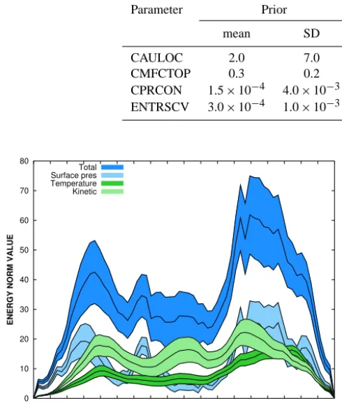
The initial distribution is defined according to expert knowledge (“Prior” in Table 2). Default model parameter val-ues provide practical valval-ues forµ₀. The initial time parame-ter uncertainties60can be set rather freely, though too small or too large uncertainties will slow down the estimation pro-cess. If no prior information about parameter correlations is available, a diagonal matrix can be used. The estimation pro-cess will reveal potential parameter covariances. Parameter bounds are also set to prevent the selection of unrealistic pa-rameter values (Table 2).

3 Total energy norm 3.1 Target criterion

The dry total energy norm in discretized form can be written as

1E=1

2

p1

X

p0

X

A

(1u)2+(1v)2+cp

Tr

(1T )2

dAdp

+1

2RdTrpr

X

A

(1lnpsfc)2dA. (2)

Here,uandvdenote the zonal and meridional wind com-ponents, T the temperature, and lnpsfc the logarithmic sur-face pressure. 1S indicates difference between two atmo-spheric states; i.e.,1S=San−Sfc, where subscripts denote analysis (an) and model forecast (fc).cp is the specific heat

at constant pressure,Rdthe gas constant of (dry) air,Tra ref-erence temperature (280 K),pra reference surface pressure (1000 hPa) and dAthe areal element of the model grid. dpis the pressure difference between two pressure levels, we use dp=1 throughout the atmosphere. Thus every model layer has the same weight in the summation. This treatment em-phasizes the surface pressure term since the correct dp val-ues in ECHAM5 with 31 vertical model levels vary between 10 and 50 hPa.

The first two terms in the right-hand side of Eq. (2) (uand

v) are identifiable as kinetic energy, and the third (T) and fourth (lnpsfc) terms as available potential energy (Lorenz, 1955, 1960). Equation (2) can also be extended to include a term related to the latent energy. We have restricted this study to the dry total energy norm. Optimal inclusion of the latent energy term requires defining a vertically changing weight-ing term (see Barkmeijer et al., 2001).

The ECMWF operational analyses are used in computa-tion of Eq. (2). The target criterion, or cost funccomputa-tion, for the EPPES estimation is then the forecast error from the analysis, the norm being the dry total energy norm.

J (θ)=w1E72(θ), (3)

where1E72denotes the energy state difference between the analysis and a 72 h forecast, andwis an ad hoc scaling term (a value of 1/6 (J/kg m2 Pa)−1 _{is used here). The scaling} term widens or narrows down the probability density func-tion (pdf) of the analysis field errors. It acts to prevent (i) that the ensemble member with the best fit to the analysis would solely affect the distribution update, and (ii) that all ensem-ble members would appear as likely. The 72 h forecast range is selected because it is beyond the tangent-linear regime of the system and not seriously affected by the spin-up/down of the model hydrology, and not yet affected by the nonlinear forecast error saturation.

3.2 Model sensitivity

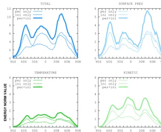
We first study (i) how the model performs in terms of energy norm, and (ii) how much impact the initial state and parame-ter perturbations have on forecasts with respect to the energy norm. Figure 1 illustrates the ensemble spread of the zonal mean energy norm at a 72 h forecast range, averaged over 15 days (1–15 January 2011). We divide the dry total energy norm (dark blue) into surface pressure (light blue), temper-ature (dark green) and kinetic energy (light green) terms in order to better understand the respective contributions to dry total energy norm variability. The width of the colored area represents±two standard deviations (SD) from the mean, thus indicating the impact of initial state and parameter per-turbations on the system. Moreover, the mean (continuous black lines) indicates how far the forecast is from the analy-ses in general.

(4)

Table 2. Parameter values for ECHAM5 (T42L31) in EPPES tests.

Parameter Prior Bounds Posterior

mean SD mean SD

CAULOC 2.0 7.0 0–30 10.79 4.29

CMFCTOP 0.3 0.2 0–1.0 0.42 0.12

CPRCON 1.5×10−4 4.0×10−3 0–1.5×10−2 3.63×10−3 1.43×10−3 ENTRSCV 3.0×10−4 1.0×10−3 0–5.0×10−3 2.12×10−4 0.91×10−4

0 10 20 30 40 50 60 70 80

90 S 60 S 30 S 0 30 N 60 N 90 N

ENERGY NORM VALUE

LATITUDE

Total Surface pres Temperature Kinetic

Figure 1. Mean error and ensemble spread of zonally averaged

and areal-weighted energy norm (unit J/kg m2Pa) for 15 days (1– 15 January 2011) from a +72 h forecast. Dry total energy norm (dark blue), and individual terms: surface pressure (light blue), tempera-ture (dark green) and kinetic energy (light green). Continuous black line indicates the mean model error. Width of the colored area rep-resents±two standard deviations from the mean.

dominate in the Southern Hemisphere, and both sources are approximately equal in the Northern Hemisphere.

The surface-pressure term has three mean error max-ima: two in the Southern Hemisphere (22 and 60◦S) and a broader one in the Northern Hemisphere (35–57◦N). The peaks at 22◦S and 35◦N, namely the Andes and the Hi-malayas regions, are caused by orographical differences be-tween ECHAM5 and the originally higher-resolution analy-sis data. Ensemble spread is the largest within the peak ar-eas of 60◦S and 40–57◦N. The southern hemispheric max-imum is dominated by initial state perturbations, whereas in the Northern Hemisphere both perturbations have an equal effect.

The temperature term has the least spread. The mean is quite flat with respect to latitude, but at higher latitudes the model deficiencies start to appear, especially in the Northern Hemisphere. The ensemble spread of the temperature term remains relatively small at all latitudes, and is governed by the initial state perturbations in the extratropics and by pa-rameter variations in the tropics.

The mean error in the kinetic energy term has also multiple maxima: one in the midlatitudes in each hemisphere, and one in the tropics. The ensemble spread is large at all latitudes. Parameter perturbations dominate the spread in the tropics and extratropics, while initial state perturbations dominate in the southern midlatitudes. In the northern midlatitudes, initial-state and parameter perturbations generate roughly the same amount of ensemble spread.

4 Results

4.1 Parameter evolution

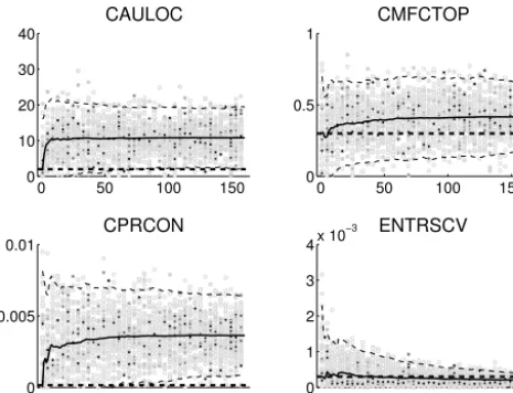
The evolution of the parameter subset from 1 January to 31 March 2011 (2011JFM) is shown in Fig. 3. The parame-ter perturbation distribution meanµ(continuous line), width (±two times the standard deviation; thin dashed lines), and default parameter values (thick dashed line) are presented. A vertical column of markers represents a set of 50 pa-rameter values evaluated at the corresponding date, and the marker shading is indicative of the importance weight in the distribution update. Two of the parameters (CAULOC and CPRCON) shift fairly quickly to higher parameter values, followed by saturation. CMFCTOP and ENTRSCV, how-ever, change more conservatively throughout the evaluation period. The posterior distribution meanµand standard devi-ation after the final iterdevi-ation are given in Table 2.

4.2 Validation 4.2.1 Skill scores

(5)

0 2 4 6 8 10 12

90S 60S 30S 0 30N 60N 90N TOTAL

per only ini only per+ini

0 1 2 3 4 5 6

90S 60S 30S 0 30N 60N 90N SURFACE PRES

0 1 2 3 4 5 6

90S 60S 30S 0 30N 60N 90N

ENERGY NORM VALUE

LATITUDE TEMPERATURE

0 1 2 3 4 5 6

90S 60S 30S 0 30N 60N 90N KINETIC

Figure 2. Ensemble spread (two times the standard deviation; unit J/kg m2Pa) at forecast day three averaged over 30 ensembles. Spread of dry total energy norm (total), and surface pressure (surface pres), temperature and kinetic energy (kinetic) terms. Experiments with only parameter perturbations active (thin continuous lines), only initial state perturbations active (dashed lines), and both sources of uncertainty active (thick continuous line).

root of number of cases) are shown. The first thing to note is that the energy norm at forecast day three for 2011JFM is im-proved at the 95% confidence level, implying that the EPPES algorithm is able to find a model that is improved with re-spect to the target criterion. In fact, there is an improvement at all ranges. The energy norm improvement is statistically significant also for forecast ranges beyond 2 days in the in-dependent sample 2011A, and beyond 5 days in the 3-month sample 2010JFM.

Next, the model is validated against the standard head-line score of 500 hPa geopotential height. In addition to the RMSE (root mean square error), the anomaly correlation co-efficient (ACC) is also shown. ACC is a verification quan-tity which is sensitive to the forecast patterns. Notation is the same in Figs. 4 and 5. Positive values for both RMSE and ACC indicate where the optimized model is performing better than the default one. The RMSE scores for all three data sets are improved at the 95 % confidence level for all forecast ranges. Interestingly, the mean RMSE scores of the independent sample of 2011A are improved more than in the dependent sample. ACC scores in the dependent sample are improved for forecast ranges longer than 2 days, and sta-tistically significantly at forecast ranges of 2.5–8 and 9.5– 10 days. The ACC scores are also improved from forecast day five onwards for the independent sample of 2011A, al-though this does not hold at the 95 % confidence level. For

the second independent sample the ACC is mostly neutral with some statistically insignificant improvements for fore-cast ranges beyond 7 days.

4.2.2 Scorecard

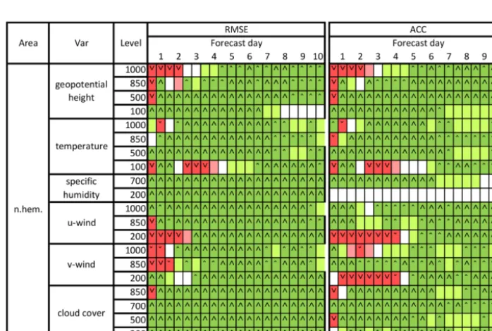
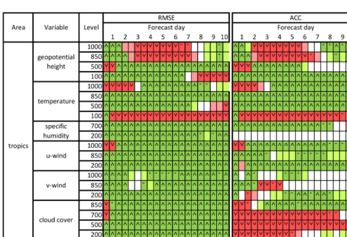
A more general validation of the model changes with the op-timized parameters is provided by a scorecard (Fig. 6a–c). It is a concise but comprehensive presentation of a large num-ber of scores for various geographical regions, variables, lev-els, and forecast ranges. The notation is such that green (red) colors indicate the optimized model scoring better (worse) than the default model. Small and large arrowheads point-ing up (down) indicate the result is significant at the 95 or 99 % confidence level, respectively, for the optimized (de-fault) model to score better. White boxes indicate the models performing equally well.

(6)

0 50 100 150 0

10 20 30 40

CAULOC

0 50 100 150 0

0.5 1

CMFCTOP

0 50 100 150 0

0.005 0.01

CPRCON

0 50 100 150 0

1 2 3 4x 10

−3 ENTRSCV

Figure 3. Evolution of parameter subsets from 1 January 2011 to

31 March 2011. The distribution meanµ(continuous line),±two times the standard deviations (thin dashed lines), and default param-eter value (thick dashed line). A vertical column of markers rep-resents parameter values evaluated at the corresponding date, the marker shading is indicative of the weighting in the distribution up-date. For clarity only every fourth ensemble is plotted.

exception of geopotential height at the forecast range of 3– 7 days at 1000 and 850 hPa levels, temperature at the 100 hPa level, and surface temperature. The ACC scores for the trop-ics are affected similarly to the RMSE scores; the exception being cloud fraction, which is negatively affected at nearly all forecast ranges.

4.2.3 Geographical validation

Next, the geographical distribution of the energy norm dif-ferences between the optimized and default models are pre-sented. The kinetic energy mean forecast difference for day three forecasts from 2011JFM is shown in Fig. 7. Positive values indicate where the optimized model is better than the default model. The main improvements are concentrated in the tropics (Southeast Asia, the western coasts of Africa and South America). A weakly positive region is close to the At-lantic storm track. The AtAt-lantic and Indian oceans around 40◦S are somewhat degraded.

Figure 8a–c illustrate the zonally averaged mean energy norm difference in the dependent sample (2011JFM) for forecast ranges of 3, 6, and 10 days (Fig. 8a–c, respec-tively). The total energy norm (dark blue), and surface pres-sure (light blue), temperature (dark green) and kinetic energy (light green) terms are presented. The mean error (continu-ous black line), and the 95 % confidence interval of the mean (width of the colored area) are also shown.

At forecast day three (Fig. 8a), most of the improvements in the dry total energy take place in the tropical belt, but there is also a favorable impact on the northern midlati-tudes (north of 45◦N). A forecast degradation is seen in the

0 100 200 300

0 1 2 3 4 5 6 7 8 9 10

2010 JFM

FORECAST DAY

0 100 200 300

0 1 2 3 4 5 6 7 8 9 10

2011 A

0 100 200 300

0 1 2 3 4 5 6 7 8 9 10

2011 JFM

Figure 4. Energy norm differences (unit J/kg m2Pa) between de-fault and optimized model. Top panel: dependent sample (January– March 2011), middle panel: independent sample of April 2011, bot-tom panel: independent sample of January–March 2010. Mean dif-ference (continuous line) and 95 % confidence interval of the mean (grey bars).

Southern Hemisphere (25–50◦_{S). In the tropics, the surface}

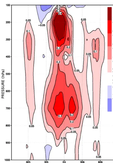
pressure term displays oscillations arising from orographi-cally induced noise as the analysis data are at higher resolu-tion than the forecasts, and the term stays negative exclud-ing the high latitudes (south of 55◦S and north of 45◦N). The temperature term displays a broad positive signal for all latitudes. Improvements in the tropics are dominated by the kinetic energy, with positive impacts for all latitudes ex-pect 25–50◦S. Figure 9 represents the vertical distribution of the zonally averaged total energy norm (EN) differences between the default and optimized model. Positive values in-dicate where the optimized model is performing better. The tropical total EN improvements seen in Fig. 8a are located between 850 and 150 hPa layers. The biggest improvements are found in the upper troposphere centered around 200 hPa, and lower in the troposphere around 700 hPa. The largest extratropical improvements occur between 400 and 300 hPa pressure levels. The southern hemispheric degradation is sit-uated near the tropopause above 100 hPa.

At longer forecast ranges, the improvements are spread from the tropics to the midlatitudes and grow larger. By fore-cast day six (Fig. 8b), the largest values are at midlatitudes and are dominated by the kinetic energy term, and later by the surface pressure term (Fig. 8c). Note the different scale in the panels of Fig. 8a–c.

5 Discussion

(7)

-0.01 -0.005 0 0.005 0.01 0.015 0.02 0.025 0.03

0 1 2 3 4 5 6 7 8 9 10 -0.5

0 0.5 1 1.5 2 2.5 3

0 1 2 3 4 5 6 7 8 9 10

2010 JFM

FORECAST DAY

-0.01 -0.005 0 0.005 0.01 0.015 0.02 0.025 0.03

0 1 2 3 4 5 6 7 8 9 10 -0.5

0 0.5 1 1.5 2 2.5 3

0 1 2 3 4 5 6 7 8 9 10

2011 A

-0.01 -0.005 0 0.005 0.01 0.015 0.02 0.025 0.03

0 1 2 3 4 5 6 7 8 9 10

ACC (OPT-DEF)

-0.5 0 0.5 1 1.5 2 2.5 3

0 1 2 3 4 5 6 7 8 9 10

2011 JFM

RMSE (DEF-OPT)

Figure 5. The 500 hPa geopotential height difference. Left panels: RMSE (default minus optimized model; unit m), right panels: ACC

(optimized minus default model). Top panels: dependent sample (January–March 2011), middle panels: independent sample of April 2011, bottom panels: independent sample of January–March 2010. Mean difference (continuous line) and 95 % confidence interval of the mean (gray bars).

Figure 6a. A forecast validation scorecard for 180 forecast cases between 1 January and 31 March 2011 for the Northern Hemisphere.

(8)

Figure 6b. As Fig. 6a, but for the Southern Hemisphere.

Figure 6c. As Fig. 6a, but for the tropics.

target criterion, and thus demonstrates that the algorithm works as intended. This improvement is not confined to the sampling period, as it is also present in the independent sam-ple 2011A, and to some extent also in the 2010JFM samsam-ple.

Figure 4 illustrates how the optimized model stays closer to the verifying analyses than the default model. The energy norm is optimized at day three but the improvements are also maintained at longer forecast ranges, and the optimized

(9)

Figure 7. Forecast day three kinetic energy mean difference (unit

J/kg m2Pa) of the optimized and default model from January to March 2011. Positive values indicate improved day three forecasts after parameter optimization.

-0.5 0 0.5 1 1.5 2

90 S 60 S 30 S 0 30 N 60 N 90 N

ENERGY NORM DIFFERENCE

LATITUDE Total

Surface pres Temperature Kinetic

Figure 8a. Zonally averaged and areal-weighted energy norm

dif-ference (unit J/kg m2Pa) between the default and optimized models from January to March 2011 for forecast day three. Dry total en-ergy norm (dark blue), and surface pressure (light blue), tempera-ture (dark green) and kinetic energy (light green) terms individually. Continuous black line indicates the mean error, and width of the col-ored area represents the 95 % confidence interval of the mean.

convective circulation in the tropics. After the 3-day opti-mization period, the tropical kinetic energy improvements spread by nonlinear model dynamics into the midlatitudes (Fig. 8b), and begin also to appear as improvements in the distribution of potential energy via the surface pressure term. Note, that there is a tropical maximum in the kinetic energy distribution at day six (Fig. 8b). The interpretation of this maximum is that the reduced model error continues to oper-ate in the tropics and feeds more realistic kinetic energy evo-lution via better tropical circulation throughout the 10-day forecast range.

-1 0 1 2 3 4

90 S 60 S 30 S 0 30 N 60 N 90 N

LATITUDE

Total Surface pres Temperature Kinetic

Figure 8b. As Fig. 8a, but for forecast day six.

0 5 10 15

90 S 60 S 30 S 0 30 N 60 N 90 N

LATITUDE Total

Surface pres Temperature Kinetic

Figure 8c. As Fig. 8a, but for forecast day 10.

(10)

Figure 9. Pressure–latitude cross section of forecast day three zonal

mean energy norm differences (unit J/kg m2Pa) between default and optimized models from January to March 2011. Positive val-ues indicate where the optimized model is performing better.

models is shown in Fig. 10. A comparison of the models re-veals that the version optimized using the energy norm is su-perior especially with respect to the winds. One reason for this result is the ambiguity of 500 hPa skill as a target: the upper troposphere and lower stratosphere circulation is not properly constrained and there are many model realizations (i.e., the same model structure at the 500 hPa level but differ-ent closure parameter values) that fulfill the target.

Analysis of the model moisture fields implies that apply-ing the moist energy norm (see e.g., Barkmeijer et al., 2001, for the formula) as the target criterion would further empha-size the tropics in the estimation process. The contribution of the moisture term to the total EN would be on the same or-der as the temperature term. We speculate that including the term into the cost function would have a small effect on the final parameter distributions. Although, without constructing a weighting function for the moisture part we cannot predict what the magnitude of the impact would actually be.

Since the target criterion can be chosen quite freely, changes in specific regions can also be targeted for optimiza-tion with the EPPES algorithm. For instance, in the current experimentations with the IFS parameter variations have a rather small impact on calculated EN scores outside the trop-ics. Thus, a cost function constructed from the tropical EN

scores might only be more efficient for optimization pur-poses.

The choice of target criterion has to be considered care-fully prior to the parameter estimation. Tuning of the physical processes could be done by e.g., focusing on the direct effects of the parametrizations only; i.e., cloudiness and precipita-tion in this study. However, this can lead to models where a (seemingly) good representation is reached at the expense of other model fields. Hence, a target criterion focusing on the model forecast skill in more general terms seems more practical when the goal of the tuning is a univocal model im-provement. The total energy norm offers a potential target for parameter optimization since it takes into account the model changes in all model fields, and focuses on key features of the model.

6 Conclusions

This article explores the use of atmospheric dry total energy norm in improving NWP model forecast skill. EPPES (Järvi-nen et al., 2012; Laine et al., 2012) is utilized to estimate four ECHAM5 model parametrization closure parameters re-lated to clouds and precipitation. The ensemble runs are gen-erated using the ECHAM5 model to evolve the perturbed ini-tial states generated by the ECMWF for their ensemble pre-diction system. Here, model error is represented (and thus ensuring sufficient spread of the ensembles) by perturbing the ECHAM5 closure parameters which are being estimated. The twice-daily 50 member ensembles are generated over a period of 3 months and each ensemble member is used in the sequential parameter distribution update according to their respective weights obtained by calculating the dry total en-ergy norm of the 3-day forecast error against the ECMWF analyses.

We first study the impact of initial state and parameter per-turbations on the ensemble spread in terms of energy norm of the 3-day forecast error in a sample of 30 forecasts using the default model. On average, the forecast departures from the analyses are largest at the Northern (winter) Hemisphere’s midlatitudes. In the tropics, the ensemble spread is mostly due to parameter variations, whereas at higher latitudes ini-tial state perturbations either dominate or are equally impor-tant as parameter perturbations.

(11)

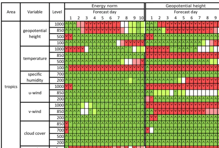
Figure 10. Comparison of forecast validation score cards for the tropics. Left column: model optimized with dry total energy norm as target

criterion, right column: model optimized with geopotential height mean squared error (MSE) at the 500 hPa level as target criterion. In total, 180 forecast cases between 1 January and 31 March 2011. Forecast performance is color coded as follows: green is good for the optimized model while red is good for the default model. Small (large) arrowhead indicates the 95 % (99 %) level of statistical significance of the score difference. The first column indicates the area; second, the variable; third, pressure level; and the fourth and fifth columns the RMSE scores for forecast days 1–10.

of tropical kinetic energy in short (up to 3-day) forecasts. This improvement spreads in 3–6-day forecasts to midlati-tudes and starts to appear as a better representation of the potential energy distribution.

We conclude that the EPPES algorithm is a viable op-tion in optimizaop-tion of atmospheric GCMs of full complex-ity. The optimization target of the algorithm can be selected rather freely. The dry total energy norm seems promising in this respect. Please note that the EPPES codes used here and some examples are available online at http://helios.fmi. fi/~lainema/eppes/.

Acknowledgements. The authors want to thank Martin Leutbecher

from ECMWF for useful discussions and help with the energy norm discretization. We are also grateful to ECMWF for the access to operational data archives. This research has been supported by the Academy of Finland project numbers 127210, 132808, 133142, and 134999. We acknowledge that the results of this research have been achieved using the PRACE-2IP project (FP7 RI-283493) resource HECToR based in the UK.

Edited by: A. Sandu

References

Barkmeijer, J., Buizza, R., Palmer, T. N., Puri, K., and Mah-fouf, J.-F.: Tropical singular vectors computed with linearized diabatic physics, Q. J. R. Meteorol. Soc., 127, 685–708, doi:10.1002/qj.49712757221, 2001.

Errico, R. M.: Interpretations of the total energy and rotational en-ergy norms applied to determination of singular vectors, Q. J. R. Meteorol. Soc., 126, 1581–1599, doi:10.1002/qj.49712656602, 2000.

Farrel, B.: Optimal excitation of neutral Rossby waves, J. Atmos. Sci., 45, 163–172, doi:10.1175/1520-0469(1988)045<0163:OEONRW>2.0.CO;2, 1988.

Gelaro, R., Buizza, R., Palmer, T. N., and Klinker, E.: Sensitivity Analysis of Forecast Errors and the Con-struction of Optimal Perturbations Using Singular Vec-tors, J. Atmos. Sci., 55, 1012–1037, doi:10.1175/1520-0469(1998)055<1012:SAOFEA>2.0.CO;2, 1998.

Järvinen, H., Räisanen, P., Laine, M., Tamminen, J., Ilin, A., Oja, E., Solonen, A., and Haario, H.: Estimation of ECHAM5 climate model closure parameters with adaptive MCMC, Atmos. Chem. Phys., 10, 9993–10002, doi:10.5194/acp-10-9993-2010, 2010. Järvinen, H., Laine, M., Solonen, A., and Haario, H.: Ensemble

pre-diction and parameter estimation system: the concept, Q. J. R. Meteorol. Soc., 138, 281–288, doi:10.1002/qj.923, 2012. Laine, M., Solonen, A., Haario, H., and Järvinen, H.: Ensemble

(12)

Lorenz, E. N.: Available potential energy and the maintenance of the general circulation, Tellus, 7, 157–167, doi:10.1111/j.2153-3490.1955.tb01148.x, 1955.

Lorenz, E. N.: Energy and numerical weather prediction, Tellus, 12, 364–373, doi:10.1111/j.2153-3490.1960.tb01323.x, 1960. Lorenz, E. N.: Predictability: A problem partly solved, in

Proceed-ings of seminar on predictability: Volume 1. ECMWF, Reading, UK, 1, 1–18, 1996.

Mitchell, H. L., Houtekamer, P., and Pellerin, G.: Ensemble Size, Balance, and Model-Error Representation in an En-semble Kalman Filter, Mon. Weather Rev., 130, 2791–2808, doi:10.1175/1520-0493(2002)130<2791:ESBAME>2.0.CO;2, 2002.

Ollinaho, P., Bechtold, P., Leutbecher, M., Laine, M., Solonen, A., Haario, H., and Järvinen, H.: Parameter variations in prediction skill optimization at ECMWF, Nonlin. Processes Geophys., 20, 1001–1010, doi:10.5194/npg-20-1001-2013, 2013a.

Ollinaho, P., Laine, M., Solonen, A., Haario, H., and Järvinen, H.: NWP model forecast skill optimization via closure pa-rameter variations, Q. J. R. Meteorol. Soc., 139, 1520–1532, doi:10.1002/qj.2044, 2013b.

Orrell, D., Smith, L., Barkmeijer, J., and Palmer, T. N.: Model error in weather forecasting, Nonlin. Processes Geophys., 8, 357–371, doi:10.5194/npg-8-357-2001, 2001.

Palmer, T. N., Buizza, R., Molteni, F., Chen, Y.-Q., and Corti, S.: Singular vectors and the predictability of weather and climate, Phil. Trans. R. Soc. Lond. A, 348, 459–475, doi:10.1098/rsta.1994.0105, 1994.

Roeckner, E., Bäuml, G., Bonaventura, L., Brokopf, R., Esch, M., Giorgetta, M., Hagemann, S., Kirchner, I., Kornblueh, L., Manzini, E., Rhodin, A., Schlese, U., Schulzweida, U., and Tompkins, A.: The atmospheric general circulation model ECHAM5, Part I: Model description, Tech. Rep. 349, Max-Planck-Institut für Meteorologie, 2003.

Schirber, S., Klocke, D., Pincus, R., Quaas, J., and Ander-son, J.: Parameter estimation using data assimilation in an atmospheric general circulation model: From a perfect to-wards the real world, J. Adv. Model Earth Syst., 5, 58–70, doi:10.1029/2012MS000167, 2013.