www.geosci-model-dev.net/7/2599/2014/ doi:10.5194/gmd-7-2599-2014
© Author(s) 2014. CC Attribution 3.0 License.
On the computation of planetary boundary-layer height using
the bulk Richardson number method
Y. Zhang1, Z. Gao2, D. Li3, Y. Li1, N. Zhang4, X. Zhao1, and J. Chen1,5
1International Center for Ecology, Meteorology & Environment, Jiangsu Key Laboratory of Agricultural Meteorology,
College of Applied Meteorology, Nanjing University of Information Science and Technology, Nanjing 210044, China
2State Key Laboratory of Atmospheric Boundary Layer Physics and Atmospheric Chemistry (LAPC),
Institute of Atmospheric Physics, Chinese Academy of Sciences, Beijing 100029, China
3Program of Atmospheric and Oceanic Sciences, Princeton University, Princeton, NJ 08540, USA 4School of Atmospheric Sciences, Nanjing University, Nanjing, 210093, China
5Department of Geography, Michigan State University, East Lansing, MI 48824, USA
Correspondence to: Z. Gao ([email protected])
Received: 15 March 2014 – Published in Geosci. Model Dev. Discuss.: 24 June 2014
Revised: 12 September 2014 – Accepted: 22 September 2014 – Published: 10 November 2014
Abstract. Experimental data from four field campaigns are used to explore the variability of the bulk Richardson num-ber of the entire planetary boundary layer (PBL), Ribc, which
is a key parameter for calculating the PBL height (PBLH) in numerical weather and climate models with the bulk Richardson number method. First, the PBLHs of three differ-ent thermally stratified boundary layers (i.e., strongly stable boundary layers, weakly stable boundary layers, and unsta-ble boundary layers) from the four field campaigns are deter-mined using the turbulence method, the potential tempera-ture gradient method, the low-level jet method, and the mod-ified parcel method. Then for each type of boundary layer, an optimal Ribcis obtained through linear fitting and
statis-tical error minimization methods so that the bulk Richard-son method with this optimal Ribc yields similar estimates
of PBLHs as the methods mentioned above. We find that the optimal Ribcincreases as the PBL becomes more unstable:
0.24 for strongly stable boundary layers, 0.31 for weakly sta-ble boundary layers, and 0.39 for unstasta-ble boundary layers. Compared with previous schemes that use a single value of Ribcin calculating the PBLH for all types of boundary
lay-ers, the new values of Ribcproposed by this study yield more
accurate estimates of PBLHs.
1 Introduction
The planetary boundary layer (PBL), or the atmospheric boundary layer, is the lowest part of the atmosphere that is directly influenced by earth’s surface and has significant im-pacts on weather, climate, and the hydrologic cycle (Stull, 1988; Garratt, 1992; Seidel et al., 2010). The height of the PBL (PBLH) is typically on the order of 1∼2 km but varies significantly during a diurnal cycle in response to changes in the thermal stratification of the PBL. It is an impor-tant parameter that is commonly used in modeling turbulent mixing, atmospheric dispersion, convective transport, and cloud/aerosol entrainment (Deardorff, 1972; Holtslag and Nieuwstadt, 1986; Sugiyama and Nasstrom, 1999; Seibert et al., 2000; Medeiros et al., 2005; Konor et al., 2009; Liu and Liang, 2010; Leventidou et al., 2013). As a result, accurate estimates of the PBLH under different thermal stratifications are critically needed.
wind profiles measured from radio soundings. In this method, the PBLs are broadly classified as strongly stable boundary layers (type I SBLs), weakly stable boundary layers (type II SBLs), or unstable boundary layers (UBLs) (Holtslag and Boville, 1993; Vogelezang and Holtslag, 1996). They are de-fined using the surface heat flux and the potential temperature profile, as shall be seen later.
For strongly stable boundary layers or type I SBLs, there is a strong inversion in the potential temperature profile and the PBLH is usually defined as the top of the inversion where the potential temperature gradient (PTG) first becomes smaller than a certain threshold γs (Bradley et al., 1993), which is
chosen to be 6.5 K 100 m−1following Dai et al. (2011). This is called the PTG method hereafter. For weakly stable bound-ary layers or type II SBLs, turbulence is generated from wind shear due to relatively high wind speed and the PBLH is de-fined as the height of the low-level jet (LLJ) (Melgarejo and Deardorff, 1974). This is called the LLJ method hereafter. For unstable boundary layers, UBLs, buoyancy is the domi-nant mechanism driving turbulence, and the PBLH is defined as the height at which a thin layer of capping inversion oc-curs. The PBLH of UBLs is determined first by identifying a height at which a parcel of dry air, released adiabatically from the surface, reaches equilibrium with its environment (Holzworth, 1964). This height is then corrected by another upward search for another height at which the potential tem-perature gradient first exceeds a thresholdγc(Liu and Liang,
2010), which is chosen to be 0.5 K 100 m−1in this study. This is called the modified parcel method hereafter.
For an atmosphere with discernible characteristics (i.e., a strongly stable potential temperature profile for the type I SBL, a strong LLJ for the type II SBL, and a capping inver-sion layer for the UBL), the three methods generally show good performance (e.g., Mahrt et al., 1979; Liu and Liang, 2010; Dai et al., 2011). However, for an atmosphere with-out these discernible characteristics, large errors can be in-troduced by these methods. As such, these methods are usu-ally used in experimental studies but not in numerical models since numerical models need to determine the PBLH auto-matically. Instead, the bulk Richardson number (Rib) method
is often used for numerical weather and climate models due to its reliability under a variety of atmospheric conditions (e.g., Holtslag and Boville, 1993; Jericevic and Grisogono, 2006; Richardson et al., 2013). The bulk Richardson num-ber method assumes that the PBLH is the height at which the Ribreaches a threshold value (Ribc, which is called “the bulk
Richardson number for the entire PBL” hereafter). The Ribat
a certain heightzis calculated with the potential temperature and wind speed at this level and those at the lower boundary of the PBL (generally the surface), as follows (Hanna, 1969):
Rib=
(g/θv0)
θvz−θv0
z
u2
z+vz2
, (1)
whereθv0 andθvz are the virtual potential temperatures at
the surface and at heightz, respectively,g/θv0 is the
buoy-ancy parameter, anduzandvzare the horizontal wind-speed
components at heightz. As can be seen from Eq. (1), the bulk Richardson number method is computationally cheap because it only requires low-frequency data. Nonetheless, the biggest challenge associated with the bulk Richardson num-ber method is that the value of Ribchas to be determined as
a prior known. In previous studies, the value of Ribc varies
from 0.15 to 1.0 (Zilitinkevich and Baklanov, 2002; Jerice-vic and Grisogono, 2006; Esau and ZilitinkeJerice-vich, 2010), with values of 0.25 and 0.5 most widely used (e.g., Troen and Mahrt, 1986; Holtslag and Boville, 1993). One important cause of the large variability of Ribcis the thermal
stratifi-cation in the PBL. For example, Vogelezang and Holtslag (1996) reported the Ribc values of 0.16–0.22 in a
noctur-nal strongly stable PBL and 0.23–0.32 in a weakly stable PBL. For unstable PBLs, a value larger than 0.25 is usually needed (Zhang et al., 2011). Esau and Zilitinkevich (2010) also showed that the Ribc for nocturnal SBLs was smaller
than for neutral and long-lived stable PBLs based on a large-eddy-simulation database. More recently, a linear relation-ship between the Ribcand the atmospheric stability
parame-ter has been proposed and examined under stable conditions, which further suggests the impact of thermal stratification on the Ribc(Richardson et al., 2013; Basu et al., 2014).
The objective of this study is to examine the variation of Ribcwith different thermal stratification conditions. To do so,
a representative value of Ribc for each type of PBLs (i.e.,
strongly stable boundary layers, weakly stable boundary lay-ers, and unstable boundary layers) needs to be inferred. In our study, the Tur method, the PTG method, the LLJ method, and the modified parcel method are used to determine the PBLHs from observations made in four field campaigns, which are called “observed” PBLHs. Using these “observed” PBLHs as benchmarks, the best choices of Ribcvalues under
differ-ent stratification conditions are then inferred so that the es-timates of PBLHs with the bulk Richardson number method match the “observed” PBLHs. These inferred values of Ribc
are used to explore the impact of thermal stratification on the Ribc.
The study is organized in the following way: Sect. 2 de-scribes the observational data used in this study; Sect. 3 compares estimates of PBLH from different methods that are widely used to determine the PBLH from measurements; Sect. 4 focuses on the bulk Richardson number method and describes the search for a best choice of Ribcunder different
stratification conditions. Section 5 concludes the paper.
2 Observational data
the Litang experiment, the Atmospheric Radiation Mea-surement (ARM) experiment, the Surface Heat Budget of the Arctic Ocean (SHEBA) experiment, and the Coopera-tive Atmosphere–Surface Exchange Study (CASES) in 1999 (CASES99). Each of these four field campaigns is briefly de-scribed as follows.
The Litang site is located over a plateau meadow in the southeast of the Tibetan Plateau. The campaign pro-vides 105 effective radio soundings of wind and tempera-ture in three observational periods (7–16 March, 13–22 May, and 7–16 July, 2008), with a typical 6 h interval (about 00:30, 06:30, 12:30, and 18:30 LST, local standard time). The 30 min averaged wind and temperature at 3 m collected by an eddy covariance system are also used for calculating the bulk Richardson number.
The ARM experiment was carried out over a plain farm-land in Shouxian, China, from 14 May to 28 December 2008. During the campaign, soundings were collected every 6 h (about 01:30, 07:30, 13:30, and 19:30 LST). Due to instru-ment malfunction, some data are excluded and a total of 842 radio soundings are retained. The 30 min averaged wind and temperature measured at 4 m by an eddy covariance sys-tem are also used.
The SHEBA site is located around the Canadian ice-breaker Dec Groseilliers in the Arctic Ocean. The data set provides radio soundings from mid-October 1997 to early October 1998. During this period, rawinsondes were re-leased 2–4 times a day (around 05:15, 11:15, 17:15, and 23:15 LST). Since the near-surface (2.5 m) data available from 29 October 1997 to 1 October 1998 at the SHEBA are hourly averages (Andreas et al., 1999; Persson et al., 2002), the surface observations and soundings do not overlap well in time. To ensure accuracy, only soundings released within 15 min around the hour were used in this study, yielding a total of 168 records.
The CASES99 is the second experiment of CASES con-ducted in Kansas, USA. The terrain is relatively flat (the average slope is about 0.5◦). In the campaign, the National Oceanic and Atmospheric Administration (NOAA) Long-EZ and Wyoming King Air accomplished the aircraft mea-surements at 50 and 25 Hz sample rates, respectively, during the period 6–27 October 1999 when the PBL was primar-ily stable. Since the lowest flight level was restricted (e.g., for security reasons), only 35 effective aircraft soundings are used in our study. The 5 min averaged near-surface (3 m) wind and temperature data recorded at the no. 16 flux tower in CASES99 (www.eol.ucar.edu/projects/cases99) are also used. The surface observations and soundings in CASES99 overlap well in time, but their horizontal positions slightly differ due to the movement of aircraft. Due to the fact that most of the sounding data from CASES99 were collected un-der strongly stable conditions and data unun-der other conditions were too limited, in this study only soundings under strongly stable conditions (i.e., in type I SBLs) are used; except in Fig. 1 where one weakly stable boundary layer case from
290 302
0 200 400 600 800 1000
Height (m)
θ (K) a2
0 5 10 15
WS (m s−1) b2
0 1 2
Rib
CASES99 (Type II SBL): 11−Oct−1999 07:38:00 LST c2 Rib Ri
bc=0.07h/L
Ri
bc=0.045h/L
−0.2 0 0.2
w’ (m s−1) d2
298 303
100 200 300 400
Height (m)
θ (K) a1
10 15
WS (m s−1) b1
0 1 2
Ri
b
CASES99 (Type I SBL): 12−Oct−1999 07:08:00 LST c1 Ri
b
Ri
bc=0.07h/L
Ri
bc=0.045h/L
−0.2 0 0.2
w’ (m s−1) d1
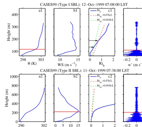
Figure 1. Examples of vertical profiles of the type I SBL (upper
panels) and the type II SBL (lower panels) from CASES99 aircraft measurements: (a) potential temperature (K); (b) horizontal wind speed (m s−1); (c) bulk Richardson number Rib and Ribc; (d) w perturbation (m s−1). The red solid lines on (a1) and (b2) denote the PBLH calculated by the PTG and LLJ methods, respectively, and those on (d) denote the PBLH determined by the Tur method. The black arrows on (c1) denote the PBLHs determined by the bulk
Richardson number method with Ribcfrom Eq. (7).
CASES99 is presented in order to compare the LLJ method to the Tur method.
In postprocessing, a 20 m moving-window average is used for all the soundings from all the sites (except the turbulence measurements by aircraft in CASES99) to remove the mea-surement noise.
3 PBLHs determined from observational data
As mentioned in the introduction, the PBLs during a typical diurnal cycle are categorized into three types: type I SBLs (i.e., strongly stable boundary layers at night), type II SBLs (i.e., weakly stable boundary layers at early morning/night), and UBLs (i.e., unstable boundary layers during the day-time). The PTG method, the LLJ method, and the modified parcel method are usually used to determine the PBLH for type I SBLs, type II SBLs, and UBLs, respectively. Based on previous studies (e.g., Holtslag and Boville, 1993; Vo-gelezang and Holtslag, 1996), they are classified using the surface heat fluxHand the potential temperatureθprofile:
H≥δ for UBLs,
H < δand d2θ/dz2<0 for type I SBLs, H < δand d2θ/dz2≥0 for type II SBLs,
whereδis the minimumHfor unstable conditions, which, in practice, is specified as a small positive value instead of zero (Liu and Liang, 2010). Due to different thermodynamic prop-erties of land and ice, the value ofδis specified as 1 W m−2 over land and 0.5 W m−2 over ice through trial and error. Under stable conditions (i.e., H < δ), the PBLs are further classified into type I SBLs and type II SBLs according to d2θ/dz2. For type I SBLs, the PTG decreases with height and the inversion near the surface is relatively strong, so there is always a sudden decrease of PTG at the PBL top (e.g., see Fig. 1a1). As such, the derivative of PTG with respect toz
should be negative; that is, d2θ/dz2<0. For type II SBLs, the PTG increases with height and the inversion is relatively weak. No sudden change of PTG is seen at the PBL top (e.g., see Fig. 1a2) and thus d2θ/dz2≥0. In this study, d2θ/dz2is calculated between 40 and 200 m; the selection of 40 m as the lower boundary is to avoid near-surface variability caused by landscape heterogeneity.
Note that cases with –δ < H < δ(i.e., under near-neutral conditions) are typically treated as type II SBL cases accord-ing to our classification. This is because stable stratification usually prevails above the boundary layer and wind shear is the only source of turbulence under near-neutral conditions. Both of these features are similar to those of a stable bound-ary layer and, as a result, the near-neutral cases are treated as SBL cases (Serbert et al., 2000). It appears there might be an abrupt change in the calculation of PBLH atH≈δif dif-ferent values of Ribcare used for SBLs and UBLs, which is
the aim of this study. However, we note that changes of Ribc
atH≈δ from SBLs to UBLs have little effect on the PBL height determination, because the Rib increases drastically
with height at the PBL top under near-neutral conditions and using Ribc for either SBLs or UBLs gives reasonable
esti-mates of PBLH (Supplementary Fig. S1).
For any of the three types of PBLs, the Tur method is the most direct and accurate approach for the PBLH estimation because it measures the turbulence intensity directly. Figure 1 shows vertical profiles of potential temperature, mean wind velocity, bulk Richardson number, and wind velocity pertur-bations from CASES99 for a type I SBL (a1–d1) and a type II SBL (a2–d2). The wind velocity perturbations (u0,v0,w0), or turbulence intensities, are obtained by removing the slowly varying part of the corresponding winds (u,v,w) through a high-pass wavelet filter (Wang et al., 1999; Wang and Wang, 2004). In the Tur method, continuous wavelet transform is applied to the absolute magnitude of turbulent fluctuations of each velocity component. The PBLH is automatically de-termined to be the level at which the absolute magnitude of these velocity fluctuations shows the most rapid decrease with height (Dai et al., 2011, 2014). The PBLHs determined byu0,v0,w0are then averaged using the absolute magnitude of the reciprocal velocity fluctuations as weights. As can be seen in Fig. 1d1 and 1d2, the PBLHs determined by the Tur method are denoted by the red solid lines.
Figure 1 further shows the PBLHs determined with the PTG method (see the red solid line on a1) and the LLJ method (see the red solid line on b2) for type I and type II SBLs, respectively. It is clear that the estimates of PBLHs with these two methods are comparable to the PBLHs deter-mined from the Tur method, suggesting that the PTG method and the LLJ method work well for type I and type II SBLs, respectively.
Figure 2 shows the sounding profiles taken from Litang on 9 July 2008 and the PBLHs estimated by the PTG, LLJ, and modified parcel methods for the three different PBLs, re-spectively. At midnight (00:35 LST), the PBL was very stable due to radiative cooling from the surface and is classified as a type I SBL. According to the PTG method, the PBLH was found at the top of the strong inversion (125 m; see Fig. 2a). In the early morning (06:35 LST), the surface temperature in-creased and thus the inversion near the surface became weak; the low-level wind speed increased rapidly and formed a LLJ. The PBL is classified as a type II SBL. With the LLJ method, the PBLH was determined at the height of the maximum wind (260 m; see Fig. 2b). As the surface heating continued, a super-adiabatic layer in which the potential temperature de-creased with height formed near the surface and a UBL was developed by midday (12:45 LST). With the modified parcel method, the PBLH is estimated to be 1654 m (see Fig. 2c). Consequently, it can be concluded that the three methods mentioned above are useful for a PBL with discernible char-acteristics (Figs. 1, 2).
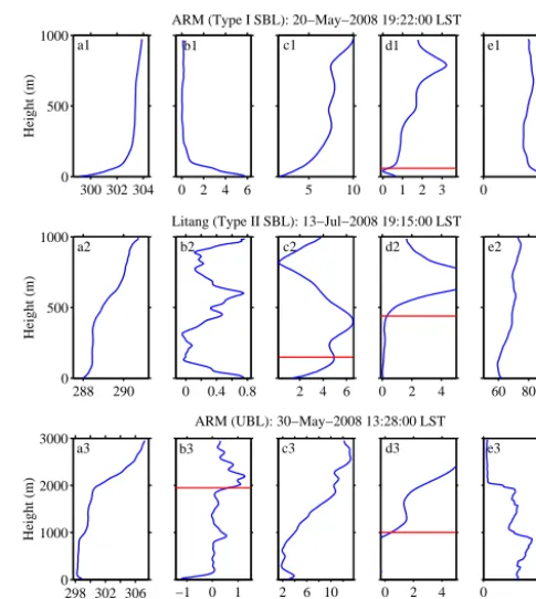
However, for a PBL without these discernible character-istics, these methods may introduce large biases (see Fig. 3 and e.g., Russell et al., 1974; Martin et al., 1988; Balsley et al., 2006; Meillier et al., 2008). For type I SBLs, when the underlying inversion is not strong, it will be difficult to determine the PBLH by the PTG method due to the fact that the maximum PTG can be less than the thresholdγs
(Fig. 3b1). For type II SBLs, when there is no clear wind-speed maximum or when multiple maxima exist, the LLJ method will have difficulties in determining the PBLH. For example, there were two maxima in the wind profile (at 160 and 400 m, see Fig. 3c2). If the PBLH is simply determined as the height where the first maximum occurs, the PBLH would be 160 m. Combining information from the Ribprofile
(Fig. 3d2), a more reasonable estimate of the PBLH should be 400 m instead of 160 m since the Ribprofile undergoes a
significant transition at 400 m. For UBLs similar complex sit-uations may occur. The results of the modified parcel method with a specified PTG threshold may be subjective since the threshold may depend on the vertical resolution and data pre-cision (Beyrich, 1997; Joffre et al., 2001). For example, there are two PTG maxima at 900 and 2000 m (see Fig. 3b3) due to the sharp drop of relative humidity at these two heights. A more accurate estimate of the PBLH should be 900 m when combining the information from the Rib profile (Fig. 3d3),
265 270 275 280 3000
2500
2000
1500
1000
500
0
Type I SBL
θ (K)
Height (m)
0 5 10
WS (m s−1)
0 2 4
Rib
280 285 290 295
Type II SBL
θ (K)
0 10 20 WS (m s−1)
0 2 4
Rib
288 290 292 294
UBL
θ (K)
0 10 20 WS (m s−1)
−2 0 2
Rib
a b c
PBLH PBLH
PBLH
Figure 2. Typical profiles of potential temperature (blue), wind
speed (red), and Rib (black) for different types of boundary
lay-ers: (a) type I SBL, (b) type II SBL, and (c) UBL. The indicated PBLHs in (a–c) are calculated by the PTG, LLJ, and modified par-cel methods, respectively. The observations in (a–c) are from Litang on 8 July 2008 16:35 UTC (00:35 LST), 8 July 2008 22:45 UTC (06:45 LST), and 9 July 2008 04:45 UTC (12:45 LST), respectively.
Although these special cases do not always exist, they limit the applications of the three methods. The accuracy of the determined PBLH can be improved with additional in-formation, as have been demonstrated before. The follow-ing sums up the procedures that are used in this study for estimating PBLH by using these four methods. First, when-ever turbulence measurements are available, the Tur method is used to determine the PBLH. Second, for type I SBL cases with a relatively weak inversion (the local PTG maxi-mum is<6.5 K(100 m)−1between 40 and 200 m), if there is a LLJ the case is reclassified to a type II SBL, if not the case is removed. Third, type II SBL cases without clear wind-speed maximum are removed. Fourth, when there are multiple wind maxima for a type II SBL or multiple PTG maxima for a UBL, the information from the Rib profile is
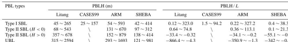
combined to determine the PBLH. With these procedures, the PBLHs obtained by using these methods are treated as “observed” PBLH hereafter. The observed PBLH and the bulk stability parameter (PBLH/L, whereL is the surface Obukhov length) for these four field experiments are pro-vided in Table 1.
4 The bulk Richardson number method and the Ribc
The PTG method, the LLJ method, and the modified par-cel method are usually used to determine the PBLH in ob-servational data. However, they do not work well when the PBL has no distinct features that are required by these meth-ods. Instead, the bulk Richardson number method with a prescribed Ribc is often used in numerical methods to
au-tomatically determine the PBLH. For example, in the non-local PBL scheme of the Community Climate Model
ver-300 302 304 0
500 1000
Height (m)
a1
0 2 4 6
b1
0 1 2 3 d1
5 10
c1
ARM (Type I SBL): 20−May−2008 19:22:00 LST
0 50
e1
288 290
0 500 1000
Height (m)
a2
0 0.4 0.8
b2
0 2 4
d2
2 4 6
c2
Litang (Type II SBL): 13−Jul−2008 19:15:00 LST
60 80 100
e2
298 302 306 0
1000 2000 3000
θv (K)
Height (m)
a3
−1 0 1
b3
θv grad. (K (100m)−1)
0 2 4
Rib d3
2 6 10
WS (m/s) c3
ARM (UBL): 30−May−2008 13:28:00 LST
0 50
RH (%) e3
Figure 3. Examples of vertical profiles in type I SBLs (upper
panels), type II SBLs (middle panels), and UBLs (lower panels):
(a) potential temperature (K), (b) potential temperature gradient
(K 100 m−1), (c) horizontal wind speed (m s−1), (d) bulk Richard-son number Rib, and (e) relative humidity (%). The red solid lines on (b3), (c2), and (d1–d3) denote the PBLH determined by the modified parcel, LLJ, and bulk Richardson number methods, re-spectively.
sion 2 (CCM2), Eq. (1) is applied to estimate the PBLH with Ribc=0.5. The computation starts by calculating the Rib
be-tween the surface and subsequent higher levels of the model. Once Ribexceeds Ribc, the PBLH is derived by a linear
in-terpolation between the level with Rib>Ribc and the level
below.
To avoid overestimating the shear production in Eq. (1) for relatively high wind speeds (i.e., in type II SBL) and to ac-count for turbulence generated by surface friction under neu-tral conditions, Vogelezang and Holtslag (1996) proposed an updated formulation, which is employed in the Community Atmosphere Model version 4 (CAM4), written as
Rib=
(g/θvs)(θvz−θvs)(z−zs)
(uz−us)2+(vz−vs)2+100u2∗
, (3)
wherezs is the height of the lower boundary for the PBL
(generally the top of the atmospheric surface layer),θvsis the
virtual potential temperature at the heightzs,usandvsare the
wind-speed components atzs.zsis often taken as 20, 40, or
Table 1. The “observed” PBLH and the stability parameter at four observational sites.
PBL types PBLH (m) PBLH /L
Litang CASES99 ARM SHEBA Litang CASES99 ARM SHEBA
Type I SBL 45∼265 25∼157 54∼593 42∼414 0.12∼323.0 1.5∼94.2 0.22∼327.2 0.4∼38.3
Type II SBL (H <0) 68∼543 \ 131∼670 97∼312 0.64∼74.8 \ 0.36∼113.1 0.1∼21.3
Type II SBL (H >0) 357∼678 \ 152∼879 138∼414 −33.4∼ −0.32 \ −34.1∼ −0.2 −55.1∼ −0.01
UBL 315∼2594 \ 293∼1693 121∼981 −866.4∼ −4.3 \ −350.9∼ −1.3 −342∼ −0.03
reaches its local minimum for UBLs. In our study, zs=40
or 80 m is used under stable conditions whilezs=0.1 PBLH
or zSAL is used under unstable conditions. The term 100u2∗
makes Eq. (3) more applicable for the near-neutral condition, which is classified as a type II SBL in our study (Seibert et al., 2000).
Under unstable conditions, the virtual potential tempera-ture at the lower boundaryθvsis replaced byθvs0 (Troen and
Mahrt, 1986; Holtslag et al., 1995):
θvs0 =θvs+bs
w0θ0 v
0
wm
, (4)
wherebs=8.5,(w0θv0)0is the virtual heat flux at the surface,
andwmis a turbulent velocity scale:
wm=
u3∗+0.6w∗3
1/3
, (5)
and
w∗=
h g
θv0
w0θ0 v
0h
i1/3
(6) is the convective velocity scale. The second term on the right-hand side of Eq. (4) represents a temperature excess, which is a measure of the strength of convective thermals.
In this study, the virtual potential temperature is estimated as the potential temperature in the calculation because the former can lead to significant fluctuations in the estimated PBLH due to inaccurate humidity measurements (Liu and Liang, 2010).
After Ribis computed from Eqs. (3)–(6), the PBLH can be
determined as the height where the Ribexceeds Ribc. In our
study, instead of calculating the PBLH using a prescribed Ribc, we infer a representative Ribc for each type of PBLs
using the “observed” PBLH (see Sect. 3) and examine the variation of the inferred Ribcwith thermal stratification. It is
pointed out here that our methodology is different from that of Richardson et al. (2013), who proposed a stability depen-dent Ribcfor SBLs:
Ribc=α
PBLH
L , (7)
where PBLH/Lis a bulk stability parameter andLis the sur-face Obukhov length.αis a proportionality constant, which
depends on surface characteristics and/or atmospheric condi-tions. It varies between 0.03 and 0.21 with suggested values of 0.045 and 0.07 (Richardson et al., 2013; Basu et al., 2014). As shown in Fig. 1c1 and c2, in the type I SBL case, a rela-tively reliable PBLH (133 m) was calculated withα=0.045, but an overestimation (184 m) occurs whenα=0.07. While in the type II SBL case bothαvalues (0.045 and 0.07) yield too small estimates of PBLH, because the two values are de-termined by idealized stable large-eddy-simulation data sets (Richardson et al., 2013) and observational data sets under weakly and moderately stable conditions (Basu et al., 2014), respectively. In addition, Eq. (7) is only applicable for SBLs but not UBLs. As such, instead of adopting this equation, we inferred a representative Ribcvalue for each type of PBL in
our study.
Because each profile provides a Ribc value, a
representa-tive Ribcat each experimental site is determined by fitting a
linear relationship between the numerator and the denomi-nator of Eq. (3) at the PBLH, as will be shown in Sect. 4.1, or using statistical error minimization methods, as will be shown in Sect. 4.2.
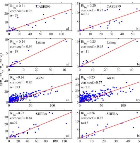
4.1 Representative Ribcfrom the linear fitting method
The representative Ribc values for type I SBLs are shown
in Fig. 4. The soundings are taken from Litang, CASES99, ARM, and SHEBA, with the heightzs of 40 (left) and 80 m
(right). Note that withzs=80 m, only cases with a PBLH ≥80 m are used. Except for CASES99, the fitted Ribc
val-ues at each site are about 0.25. The difference in Ribcwhen
different values forzs (40 or 80 m) are used is small.
How-ever, the results are slightly more consistent withzs=40 m
compared tozs=80 m, as can be seen from the higher
cor-relation coefficients at ARM and CASES99. The value of Ribcfor type I SBLs from CASES99 aircraft measurements is
0 10 20 30 40 0
5 10
Ri bc= 0.24 corr.coef.= 0.94 n= 19
Litang
a2
0 10 20 30 40
0 5 10 Ri
bc= 0.25 corr.coef.= 0.95 n= 11
Litang
b2
0 20 40 60 80 100
0 10 20 30 Ri
bc= 0.21 corr.coef.= 0.78 n= 29
CASES99
a1
0 10 20 30 40 50
0 5 10 15
Ribc= 0.20 corr.coef.= 0.73 n= 21
CASES99
b1
0 50 100
0 20 40
Ribc=0.26 corr.coef.= 0.85 n= 373 ARM (g/ θvs ) ⋅ ( θvh − θvs ) ⋅ (h−z s ) a3
0 50 100
0 10 20 30 40Ribc=0.25
corr.coef.=0.77 n= 211
ARM
b3
0 20 40 60 80 100 120
0 10 20 30
Ribc=0.27
n=27 corr.coef.= 0.84
SHEBA
(u h−us)
2 +(v
h−vs) 2
+100 u * 2
a4
0 10 20 30 40 50
0 5 10 15 Ri bc=0.26 n=17 corr.coef.= 0.87 SHEBA (u h−us)
2 +(v
h−vs) 2
+100 u * 2
b4
Figure 4. Linear fitting method inferred Ribcfor type I SBLs, with zs=40 m (left) andzs=80 m (right). The red solid lines are the best linear fittings and their slopes represent the values of Ribc.
The inferred Ribc values for type II SBLs are shown in
Fig. 5. Compared to the results in Fig. 4, the correlation coefficients in Fig. 5 are smaller, indicating that the PBLH is more difficult to determine for weakly stable boundary layers, which is consistent with previous studies (e.g., Esau and Zilitinkevich, 2010). The correlation coefficients indi-cate that the agreement withzs=80 m is slightly better than
withzs=40 m. In particular, the inferred Ribcis sensitive to
the heightzsin the SHEBA data. It changes from 0.21 to 0.29
as the heightzschanges from 40 to 80 m. The main cause of
the large variation of Ribcis because the LLJs above the ice
surface in SHEBA are considerably strong (up to 20 m s−1) and the vertical wind-speed gradients are large, so the de-nominator in Eq. (3) decreases more rapidly with the height
zsthan the numerator, which leads to an increase in the Ribc
value whenzsincreases from 40 to 80 m. However, the Ribc
over land varies little with zs (Fig. 5), which is consistent
with the findings of Vogelezang and Holtslag (1996) using the Cabauw data.
For UBLs, the height zs is chosen to be 0.1 PBLH (left)
andzSAL(right) in Fig. 6. As can be seen, the correlation
co-efficients are smaller than 0.4 at all sites, implying large vari-ability in the Ribcinferred from each sounding. The
represen-tative value of Ribcis larger than 0.25 and varies from 0.28
to 0.34. However, it appears that the PBLH estimated by the bulk Richardson number method seems to be less sensitive to Ribcunder unstable conditions. The estimates of PBLH using
the bulk Richardson number method with Ribc=0.25 or 0.5
are both in good agreement with the “observed” PBLH at the
0 20 40 60 80
0 10 20 30 Ri bc=0.27 n=53 corr.coef.= 0.75 Litang a1
0 10 20 30 40 50 60
0 10 20
Ribc=0.26
n=53 corr.coef.= 0.78
Litang
b1
0 50 100 150 200 250 300 0
50 100 Ribc=0.25
n=194 corr.coef.= 0.72 ARM (g/ θvs ) ⋅ ( θvh − θvs ) ⋅ (h−z s ) a2
0 50 100 150 200 250
0 50 100 Ribc=0.27
n=194 corr.coef.= 0.72
ARM
b2
0 100 200 300
0 20 40 60 80 Ri bc=0.21 n=49 corr.coef.= 0.79 SHEBA
(uh−us)2+(vh−vs)2+100 u*2 a3
0 50 100 150 200 250
0 20 40 60 Ribc=0.29
n=49 corr.coef.= 0.86
SHEBA
(uh−us)2+(vh−vs)2+100 u*2 b3
Figure 5. Linear fitting method inferred Ribcfor type II SBLs, with zs=40 m (left) andzs=80 m (right). The red solid lines are the best linear fittings and their slopes represent the values of Ribc.
0 50 100 150 200 250
0 50 100
150 Ribc=0.29
n=23 corr.coef.= 0.17 Litang
a1
0 50 100 150 200 250 300 0
50 100
150 Ribc=0.28
n=23 corr.coef.= 0.21 Litang
b1
0 50 100 150 200
0 50 100 Ri bc=0.30 n=182 corr.coef.= 0.19 ARM (g/ θvs ) ⋅ ( θvh − θvs ) ⋅ (h−z s ) a2
0 50 100 150
0 50 100 Ri bc=0.34 n=182 corr.coef.= 0.24 ARM b2
0 20 40 60 80
0 10 20 30 Ri bc=0.28 n=62 corr.coef.= 0.36 SHEBA (u h−us)
2 +(v
h−vs) 2
+100 u * 2
a3
0 20 40 60 80
0 10 20 30 Ri bc=0.33 n=75 corr.coef.= 0.37 SHEBA (u h−us)
2 +(v
h−vs) 2
+100 u * 2
b3
Figure 6. Linear fitting method inferred Ribcfor UBLs, withzs= 0.1 PBLH (left) andzs=zSAL (right). The red solid lines are the best linear fittings and their slopes represent the values of Ribc.
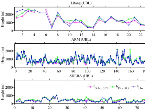
three sites (Fig. 7). This is also in agreement with some pre-vious studies (Troen and Mahrt, 1986). Therefore, the bulk Richardson number method is still reliable in estimating the PBLH of UBLs, despite the inferred Ribcshowing large
vari-ability.
4.2 Representative Ribcfrom the error minimization
method
2 4 6 8 10 12 14 16 18 20 22 0
1000 2000
Height (m)
Litang (UBL)
0 20 40 60 80 100 120 140 160 180
0 1000 2000
Height (m)
ARM (UBL)
0 10 20 30 40 50 60 70
0 1000 2000
Height (m)
SHEBA (UBL)
Sounding number h
Ribc=0.25 hRibc=0.5 hobs
Figure 7. Comparisons of the heights of UBL at different sites
de-termined by the bulk Richardson number method with Ribc=0.25
(diamond) and 0.5 (circle), and the observed PBLHs (point).
disadvantages. For example, the inferred value of Ribc and
the correlation coefficients highly depend on the larger value points, while the impact of the smaller value points is re-duced (see e.g., Fig. 4a2). Therefore, we apply error min-imization methods in this section to determine the optimal Ribc. The values of Ribcbetween 0.1–0.4 in stable conditions
and 0.2–0.5 in unstable conditions are first used to calculate the PBLH; then, three statistical measures are used to exam-ine the accuracy of the estimated PBLH (Gao et al., 2004):
bias= n
P
i=1
hRib−hobs
n , (8)
SEE=
v u u u t
n
P
i=1
hRib−hobs
2
n−2 , (9)
NSEE=
v u u u u u u t
n
P
i=1
hRib−hobs
2
n
P
i=1
(hobs)2
, (10)
wherehRib is the estimated PBLH by the bulk Richardson
number method, and hobs represents the observed PBLH
(i.e., calculated using the Tur, PTG, LLJ, or modified parcel method). Bias, SEE, and NSEE are the absolute bias, stan-dard error, and normalized stanstan-dard error ofhRibagainsthobs,
respectively, andnis the sampling number. Optimal values of Ribccan be determined based on the minimum bias, SEE,
and NSEE. Note that the optimal Ribcdetermined based on
the minimum bias, or the minimum SEE/NSEE can be dif-ferent, however, the minimum SEE and the minimum NSEE always yield the same optimal Ribc. In this study, minimum
SEE and NSEE are used as the final criterion for the optimal
Ribc. To compare the error minimization method with the
lin-ear fitting method, the correlation coefficients betweenhobs
andhRib are also presented.
The correlation coefficient, bias, SEE, and NSEE with dif-ferent values of Ribcfor type I SBLs are shown in Fig. 8 when
zs=40 (top panels) and 80 m (bottom panels). Quadratic
curves are fitted to these data and then the maximum or min-imum of the fitted quadratic curves are obtained, which are used to select the optimal Ribc for each site. The weighted
averages based on the sampling number at the four sites are treated as the representative optimal Ribcacross the four sites
(see the black dashed lines in Fig. 8) and the error bars depict the range of the optimal Ribcacross the four sites (Fig. 8).
The variability of the optimal Ribcvalues for different sites
is probably caused by the diversity of surface characteris-tics (e.g., surface roughness). Compared to the results with
zs=80 m, the error bars are smaller and thus the optimal Ribc
across different sites are more concentrated withzs=40 m.
Furthermore, the maximum correlation coefficient is larger and the minimum bias, SEE, and NSEE are smaller with
zs=40 m.
Compared to type I SBLs, the correlation coefficients are smaller and errors are larger for type II SBLs (Fig. 9), again indicating that the PBLH for weakly stable boundary lay-ers is more difficult to determine. However, the maximum correlation coefficient, minimum bias, SEE and NSEE, and the range of optimal Ribcshow smaller differences between
different values ofzs (40 or 80 m). Compared to the results
of the linear fitting method, the values of Ribcare generally
larger for each site, which is understandable given that the scatter distribution is mostly above the fitted lines in Fig. 5, especially at ARM and SHEBA. The optimal Ribcbased on
minimum SEE and NSEE for type II SBLs is 0.30–0.31. The result is consistent with the value (i.e., 0.3) from Melgarejo and Deardorff (1974).
For UBLs, Fig. 10 shows that the maximum correlation coefficient is larger, the minimum bias, SEE, and NSEE are smaller, and the values of optimal Ribcfor each site are more
concentrated with zs=zSAL (bottom panels) compared to
zs=0.1 PBLH (top panels). Therefore,zSALis more
appro-priate as the lower boundary height in estimating the PBLH under unstable conditions. The minimum SEE and NSEE indicate that the optimal Ribcis 0.39 under unstable
condi-tions. The results with zs=40 or 80 m are also examined
but not shown here. The maximum correlation coefficient and minimum bias, SEE, and NSEE are close to those with
zs=0.1 PBLH, but the values of the optimal Ribcare more
scattered across different sites.
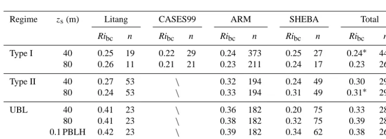
Through the above statistical error minimization methods, the optimal Ribcfor different stratifications and sites with
dif-ferent choices of zs are summarized in Table 2. It appears
that the optimal Ribc value increases when the PBL
stabil-ity decreases (i.e., as the PBL becomes more unstable). The optimal Ribc value is 0.24 (zs=40 m) or 0.23 (zs=80 m)
0.7 0.8 0.9 1
a1
Corr.coef.
10 20 30 40 50 60 70
b1
Bias
20 40 60 80 100
c1
SEE
0.1 0.2 0.3 0.4 0.5 0.6
NSEE
d1
CASE99 Litang ARM SHEBA
0.7 0.8 0.9 1
0.1 0.2 0.3 0.4
a2
Corr.coef.
Ri bc
10 20 30 40 50 60 70
0.1 0.2 0.3 0.4
b2
Bias
Ri bc
20 40 60 80 100
0.1 0.2 0.3 0.4
c2
SEE
Ri bc
0.1 0.2 0.3 0.4 0.5 0.6
0.1 0.2 0.3 0.4
d2
NSEE
Ri bc
Figure 8. Comparison between estimated PBLH using the bulk Richardson number method withzs=40 m (upper panels) andzs=80 m (lower panels) and observed PBLHs for type I SBLs. The correlation coefficient (a), bias (b), standard error (c), and normalized standard error (d) are shown. The sounding data are taken from Litang (plus sign), CASES99 (square), ARM Shouxian (diamond), and SHEBA (pentacle). The curved lines are obtained by quadratic curve-fitting, the black vertical dashed lines indicate a representative Ribcfor all four sites, and the error bars indicate the range of Ribcacross the four sites.
0.7 0.8 0.9 1
a1
Corr.coef.
20 40 60 80 100 120 140
b1
Bias
50 100 150 200
c1
SEE
0.25 0.3 0.35 0.4 0.45 0.5
NSEE
d1
Litang ARM SHEBA
0.7 0.8 0.9 1
0.1 0.2 0.3 0.4
a2
Corr.coef.
Ribc
20 40 60 80 100 120 140
0.1 0.2 0.3 0.4
b2
Bias
Ribc
50 100 150 200
0.1 0.2 0.3 0.4
c2
SEE
Ribc
0.25 0.3 0.35 0.4 0.45 0.5
0.1 0.2 0.3 0.4
d2
NSEE
Ribc
Figure 9. Comparison between estimated PBLHs using the bulk Richardson number method withzs=40 m (upper panels) andzs=80 m (lower panels) and observed PBLHs for type II SBLs. The correlation coefficient (a), bias (b), standard error (c), and normalized standard error (d) are shown. The sounding data are taken from Litang (plus sign), ARM Shouxian (diamond), and SHEBA (pentacle). The curved lines are obtained by quadratic curve-fitting, the black vertical dashed lines indicate a representative Ribcfor all three sites, and the error bars indicate the range of Ribcacross the three sites.
for type II SBLs. For UBLs, the optimal Ribcvalue falls
be-tween 0.33 and 0.39, depending on the choice of zs. To be
exact, the best choices of Ribc suggested by this study are
0.24 (zs=40 m), 0.31 (zs=80 m), and 0.39 (zs=zSAL) for
type I SBLs, type II SBLs, and UBLs, respectively. Note that
zs is recommended to be 80 m for type II SBLs, given that
the surface layer is usually thicker for type II SBLs than for type I SBLs.
4.3 Impacts of thermal stratification on Ribc
With the above analyses, the best choices of Ribcare inferred
under different thermal stratification conditions. Hence, the traditional way of determining the PBLH using a sin-gle value of Ribc without considering the dependence of
Ribcon thermal stratification (e.g., Troen and Mahrt, 1986)
0.7 0.8 0.9 1
a1
Corr.coef.
100 120 140 160 180 200
b1
Bias
150 200 250 300
c1
SEE
0.2 0.22 0.24 0.26 0.28 0.3
NSEE
d1
Litang ARM SHEBA
0.7 0.8 0.9 1
0.2 0.3 0.4 0.5
a2
Corr.coef.
Ri bc
100 120 140 160 180 200
0.2 0.3 0.4 0.5
b2
Bias
Ri bc
150 200 250 300
0.2 0.3 0.4 0.5
c2
SEE
Ri bc
0.2 0.22 0.24 0.26 0.28 0.3
0.2 0.3 0.4 0.5
d2
NSEE
Ri bc
Figure 10. Comparison between estimated PBLHs using the bulk Richardson number method with zs=0.1 PBLH (upper panels) and zs=zSAL(lower panels) and observed PBLHs for UBLs. The correlation coefficient (a), bias (b), standard error (c), and normalized standard error (d) are shown. The sounding data are taken from Litang (plus sign), ARM Shouxian (diamond), and SHEBA (pentacle). The curved lines are obtained by quadratic curve-fitting, the black vertical dashed lines indicate a representative Ribcfor all three sites, and the error bars indicate the range of Ribcacross the three sites.
Table 2. Inferred bulk Richardson number of the entire PBL, Ribc, for different types of PBLs and sites, with different values ofzs.nrefers to the sample number.∗indicates the best choice.
Regime zs(m) Litang CASES99 ARM SHEBA Total
Ribc n Ribc n Ribc n Ribc n Ribc n
Type I 40 0.25 19 0.22 29 0.24 373 0.25 27 0.24∗ 448
80 0.26 11 0.21 21 0.23 211 0.24 17 0.23 261
Type II 40 0.27 53 \ 0.32 194 0.24 49 0.30 296
80 0.24 53 \ 0.33 194 0.31 49 0.31∗ 296
UBL 40 0.41 23 \ 0.36 182 0.20 75 0.33 280
80 0.41 23 \ 0.38 182 0.32 75 0.39 280
0.1 PBLH 0.42 23 \ 0.39 182 0.34 62 0.38 267
zSAL 0.39 23 \ 0.41 182 0.36 75 0.39∗ 280
(YSU) PBL scheme in the Weather Research and Forecasting (WRF) model assumes Ribc=0.25 over land (Hong, 2010),
while Ribc=0.5 is used in the Holtslag and Boville (HB)
boundary-layer scheme in CCM2 (Holtslag and Boville, 1993). To examine the impact of thermal stratification on Ribc, we obtained a single representative Ribcfor all
strati-fication conditions with the same sounding data from Litang, ARM, and SHEBA sites, assuming the lower boundary heightszs of 40 and 80 m, andzSAL for type I SBLs, type II
SBLs, and UBLs, respectively. According to the minimum SEE and NSEE, the optimal choice of Ribcfor all PBL types
is 0.33 (Fig. 11), which is close to that used in CAM4 (Ribc=
0.3; Neale et al., 2010). In Fig. 12, the errors that occur when a single value of Ribcis used (Ribc=0.33 determined
by our study, Ribc=0.25 in WRF–YSU, and Ribc=0.5 in
CCM2–HB) are presented, as compared to the errors with a new scheme that uses Ribc=0.24, 0.31, and 0.39 for type I
SBLs, type II SBLs, and UBLs, respectively. It is found that the new scheme with variable Ribc is more reliable in
es-timating PBLH, suggesting that the impact of atmospheric stability or thermal stratification on Ribc is significant and
that the variation of Ribc with atmospheric stability should
be taken into account when estimating the PBLH using the bulk Richardson number method.
To further investigate the improvements in estimating PBLHs with the new, variable Ribc values, simulations
us-ing CAM4 are conducted at the ARM site, with the default (i.e., 0.3) and the new, variable Ribcvalues used to estimate
0.65 0.7 0.75 0.8 0.85 0.9 0.95
0.1 0.2 0.3 0.4 0.5
a
Corr.coef.
Ri bc
60 80 100 120 140
0.1 0.2 0.3 0.4 0.5
b
Bias
Ri bc
140 160 180 200 220 240 260
0.1 0.2 0.3 0.4 0.5
c
SEE
Ri bc
0.2 0.25 0.3 0.35 0.4 0.45
0.1 0.2 0.3 0.4 0.5
NSEE
Ri bc
d
Litang ARM SHEBA
Figure 11. Comparison between estimated PBLH using the bulk Richardson number method and observed PBLHs for all types of PBLs.
The correlation coefficient (a), bias (b), standard error (c), and normalized standard error (d) are shown. The sounding data are taken from Litang (plus sign), ARM Shouxian (diamond), and SHEBA (pentacle). The curved lines are obtained by quadratic curve-fitting, the black vertical dashed lines indicate a representative Ribcfor all three sites, and the error bars indicate the range of Ribcacross the three sites.
0 50 100 150
Bias
Litang ARMSHEBATotal
a
0 50 100 150 200 250
SEE
Litang ARMSHEBATotal
b
0 0.1 0.2 0.3 0.4
NSEE
Litang ARMSHEBATotal
c
New Ribc=0.33
YSU HB
Figure 12. Comparisons between observed and estimated PBLHs
with a single Ribc=0.33 for all PBL conditions, with Ribc=0.25
as in the YSU scheme, with Ribc=0.5 as in the HB scheme, and
with the new, variable values (Ribc=0.24, 0.31, and 0.39 for type I SBLs, type II SBLs, and UBLs, respectively): (a) bias, (b) standard error, (c) normalized standard error.
Ribcvalues over a 6-day period. It can be seen that the
sim-ulated PBLHs with the new Ribc values have a more
pro-nounced diurnal cycle, which are also closer to the obser-vations. Over the whole observational period, results indi-cate that the bias, SEE, and NSEE are 270.1 m, 379.3 m, and 0.75 with the new, variable Ribcvalues, respectively, and
306.2 m, 417.5 m, 0.83 with the default Ribc value,
respec-tively. Again, these results indicate that the impact of ther-mal stratification on Ribcshould be considered in calculating
PBLH with the bulk Richardson number method and that the new Ribcvalues determined in this study improve model
re-sults in real applications. It is pointed out here that there are still large biases in the CAM4-simulated PBLH even with the new Ribcvalues, which are probably related to the biases
in the model physics and parameterizations (e.g., parameter-izations of land–atmosphere interactions and boundary-layer turbulence). Unraveling how biases in the model physics and parameterizations affect the PBLH is nevertheless out of the scope of this study.
290 291 292 293 294
0 500 1000 1500 2000
Day of Year
Height (m)
Obs
CAM4 (default) CAM4 (new)
Figure 13. Comparison of observed and simulated PBLHs using
CAM4 with the default and new Ribc values during the period
16–21 October 2008 at the ARM site.
5 Conclusions
and CASES99 field experiments. The estimated PBLHs us-ing these methods are treated as observed PBLHs.
The bulk Richardson number method is more commonly used in numerical models due to its reliability for all at-mospheric stratification conditions, which requires a spec-ified value of the bulk Richardson number for the entire PBL, or Ribc. In many numerical models, the Ribc is
spec-ified as one single value (e.g., 0.25 for WRF–YSU, 0.5 for CCM2–HB, 0.3 for CAM4) and hence its dependence on the thermal stratification is ignored. This study infers a repre-sentative Ribcfor each stratification condition from observed
PBLHs using linear fitting and statistical error minimization approaches. Results indicate that the best choices for Ribc
are 0.24, 0.31, and 0.39 for strongly stable boundary layers (type I SBLs), weakly stable boundary layers (type II SBLs), and unstable boundary layers (UBLs), respectively. Both of-fline and online evaluations show that the new and variable Ribc values proposed in this study yield more reliable
es-timates of the PBLH, suggesting that the variation of Ribc
should be considered when computing the PBLH with the bulk Richardson number method.
The Supplement related to this article is available online at doi:10.5194/gmd-7-2599-2014-supplement.
Acknowledgements. This study is supported by the China
Meteoro-logical Administration under grant GYHY201006024, the National Program on Key Basic Research Project of China (973) under grants 2012CB417203 and 2011CB403501, the National Natural Science Foundation of China under grant 41275022, and the CAS Strategic Priority Research Program, grant 5 XDA05110101. We are grateful to two anonymous reviewers for their careful review and valuable comments, which led to a substantial improvement of this manuscript.
Edited by: A. Colette
References
Andre, J. C. and Mahrt, L.: The nocturnal surface inversion and influence of clear-air radiative cooling, J. Atmos. Sci., 39, 864–878, 1982.
Andreas, E. L., Fairall, C. W., Guest, P. S., and Persson, P. O. G.: An overview of the SHEBA atmospheric surface flux program, in: Preprints, Fifth Conference On Polar Meteorology and Oceanog-raphy, 10–15 January 1999, Dallas, TX, American Meteorologi-cal Society, Boston, 411–416, 1999.
Balsley, B. B., Frehlich, R. G., Jensen, M. L., and Meillier, Y.: High-resolution in situ profiling through the stable boundary layer: Examination of the SBL top in terms of minimum shear, max-imum stratification, and turbulence decrease, J. Atmos. Sci., 63, 1291–1307, 2006.
Basu, S., Holtslag, A. A. M., Caporaso, L., Riccio, A., and Steen-eveld, G. J.: Observational support for the stability dependence of the bulk Richardson number across the stable boundary layer, Bound.-Lay. Meteorol., 150, 515–523, doi:10.1007/s10546-013-9878-y, 2014.
Beyrich, F.: Mixing height estimation from sodar data-a critical dis-cussion, Atmos. Environ., 31, 3941–3954, 1997.
Bradley, R. S., Keimig, F. T., and Diaz, H. F.: Recent changes in the North American Arctic boundary layer in winter, J. Geophys. Res., 98, 8851–8858, doi:10.1029/93JD00311, 1993.
Dai, C., Wang, Q., Kalogiros, J. A., Lenschow, D. H., Gao, Z., and Zhou, M.: Determining boundary-layer height from aircraft measurements, Bound.-Lay. Meteorol., 152, 277–302, doi:10.1007/s10546-014-9929-z, 2014.
Dai, C. Y., Gao, Z. Q., Wang, Q., and Cheng, G.: Analysis of at-mospheric boundary layer height characteristics over the Arctic Ocean using the aircraft and GPS soundings, Atmospheric and Oceanic Science Letters, 4, 124–130, 2011.
Deardorff, J. W.: Parameterization of the planetary boundary layer for use in general circulation models, Mon. Weather Rev., 100, 93–106, 1972.
Esau, I. and Zilitinkevich, S.: On the role of the planetary bound-ary layer depth in the climate system, Adv. Sci. Res., 4, 63–69, doi:10.5194/asr-4-63-2010, 2010.
Gao, Z., Chae, N., Kim, J., Hong, J., Choi, T., and Lee, H.: Modeling of surface energy partitioning, surface temperature, and soil wetness in the Tibetan prairie using the Simple Biosphere Model 2 (SiB2), J. Geophys. Res., 109, D06102, doi:10.1029/2003JD004089, 2004.
Garratt, J. R.: The atmospheric boundary layer, Cambridge Univer-sity Press, 316 pp., 1992.
Hanna, S. R.: The thickness of the planetary boundary layer, Atmos. Environ., 3, 519–536, 1969.
Holtslag, A. A. M. and Boville, B. A.: Local versus nonlocal boundary-layer diffusion in a global climate model, J. Climate, 6, 1825–1842, 1993.
Holtslag, A. A. M. and Nieuwstadt, F. T. M.: Scaling the atmo-spheric boundary layer, Bound.-Lay. Meteorol., 36, 201–209, 1986.
Holtslag, A. A. M., van Meijgaard, E., and de Rooy, W. C.: A com-parison of boundary layer diffusion schemes in unstable condi-tions over land, Bound.-Lay. Meteorol., 76, 69–95, 1995. Holzworth, C. G.: Estimates of mean maximum mixing depths in
the contiguous United States, Mon. Weather Rev., 92, 235–242, 1964.
Hong, S.-Y.: A new stable boundary-layer mixing scheme and its impact on the simulated East Asia summer monsoon, Q. J. Roy. Meteor. Soc., 136, 1481–1496, 2010.
Jericevic, A. and Grisogono, B.: The critical bulk Richardson num-ber in urban areas: verification and application in a numerical weather prediction model, Tellus A, 58, 19–27, 2006.
Joffre, S. M., Kangas, M., Heikinheimo, M., and Kitaigorod-skii, S. A.: Variability of the stable and unstable atmospheric boundary-layer height and its scales over a boreal forest, Bound.-Lay. Meteorol., 99, 429–450, 2001.
Leventidou, E., Zanis, P., Balis, D., Giannakaki, E., Pytharoulis, I., and Amiridis, V.: Factors affecting the comparisons of plan-etary boundary layer height retrievals from CALIPSO, ECMWF and radiosondes over Thessaloniki, Greece, Atmos. Environ., 74, 360–366, 2013.
Liu, S. and Liang, X. Z.: Observed diurnal cycle climatology of planetary boundary layer height, J. Climate, 23, 5790–5809, doi:10.1175/2010JCLI3552.1, 2010.
Mahrt, L., Heald, R. C., Lenschow, D. H., Stankov, B. B., and Troen, I.: An observational study of the nocturnal boundary layer, Bound.-Lay. Meteorol., 17, 247–264, 1979.
Martin, C. L., Fitzjarrald, D., Garstang, M., Oliveira, A. P., Greco, S., and Browell, E.: Structure and growth of the mixing layer over the Amazonian rain forest, J. Geophys. Res., 93, 1361–1375, 1988.
Medeiros, B., Hall, A., and Stevens, B.: What controls the cli-matological depth of the PBL?, J. Climate, 18, 2877–2892, doi:10.1175/JCLI3417, 2005.
Meillier, Y. P., Froehlich, R. G., Jones, R. M., and Balsley, B. B.: Modulation of small-scale turbulence by ducted gravity waves in the nocturnal boundary layer, J. Atmos. Sci., 65, 1414–1427, 2008.
Melgarejo, J.‘W. and Deardorff, J. W.: Stability functions for the layer resistance laws based upon observed boundary-layer heights, J. Atmos. Sci., 31, 1324–1333, 1974.
Neale, R. B., Richter, J. H., Conley, A. J., Park, S., Lauritzen, P. H., Gettelman, A., Williamson, D. L., Rasch, P. J., Vavrus, S. J., Tay-lor, M. A., Collins, W. D., Zhang, M., and Lin, S.-J.: Descrip-tion of the NCAR Community Atmosphere Model (CAM 4.0), NCAR/TN-485+STR NCAR, Boulder, CO, 224 pp., 2010. Persson, P. O. G., Fairall, C. W., Andreas, E. L, Guest, P. S.,
and Perovich, D. K.: Measurements near the atmospheric sur-face flux group tower at SHEBA: Near-sursur-face conditions and surface energy budget, J. Geophys. Res., 107, 8045, doi:10.1029/2000JC000705, 2002.
Richardson, H., Basu, S., and Holtslag, A. A. M.: Improving sta-ble boundary-layer height estimation using a stability-dependent critical bulk Richardson number, Bound.-Lay. Meteorol., 148, 93–109, doi:10.1007/s10546-013-9812-3, 2013.
Russell, P. B., Uthe, E. E., Ludwig, F. L., and Shaw, N. A.: A comparison of atmospheric structure as observed with monos-tatic acoustic sounder and lidar techniques, J. Geophys. Res., 79, 5555–5566, 1974.
Seibert, P., Beyrich, F., Gryning, S. E., Joffre, S., Rasmussen, A., and Tercier, P.: Review and intercomparison of operational meth-ods for the determination of the mixing height, Atmos. Environ., 34, 1001–1027, 2000.
Seidel, D. J., Ao, C. O., and Li, K.: Estimating climatological plane-tary boundary layer heights from radiosonde observations: Com-parison of methods and uncertainty analysis, J. Geophys. Res., 115, D16113, doi:10.1029/2009JD013680, 2010.
Stull, R. B.: An introduction to boundary layer meteorology, Kluwer Academic, 666 pp., 1988.
Sugiyama, G. and Nasstrom, J. S.: Methods for Determining the Height of the Atmospheric Boundary Layer, UCRL-ID-133200, Lawrence Livermore National Laboratory Report, February 1999.
Troen, I. and Mahrt, L.: A simple model of the planetary boundary layer: Sensitivity to surface evaporation, Bound.-Lay. Meteorol., 37, 129–148, 1986.
Vogelezang, D. H. P. and Holtslag, A. A. M.: Evaluation and model impacts of alternative boundary-layer height formulations, Bound.-Lay. Meteorol., 81, 245–269, doi:10.1007/BF02430331, 1996.
Wang, Q. and Wang, S.: Turbulent and thermodynamic structure of the autumnal arctic boundary layer due to embedded clouds, Bound.-Lay. Meteorol., 113, 225–247, 2004.
Wang, Q., Lenschow, D. H., Pan, L., Schillawski, R. D., Kok, G. L., Prevot, A. S. H., Laursen, K., Russell, L. M., Bandy, A. R., Thornton, D. C., and Suhre, K.: Characteristics of the marine boundary layers during two Lagrangian measurement periods: 2. Turbulence structure, J. Geophys. Res., 104, 21767–21784, 1999.
Zilitinkevich, S. S. and Baklanov, A.: Calculation of the height of stable boundary layers in practical applications, Bound.-Lay. Meteorol., 105, 389–409, 2002.