www.geosci-model-dev.net/7/3111/2014/ doi:10.5194/gmd-7-3111-2014
© Author(s) 2014. CC Attribution 3.0 License.
A simplified permafrost-carbon model for long-term climate studies
with the CLIMBER-2 coupled earth system model
K. A. Crichton1,2, D. M. Roche3,4, G. Krinner1,2, and J. Chappellaz1,2 1CNRS, LGGE (UMR5183), 38041 Grenoble, France
2Univ. Grenoble Alpes, LGGE (UMR5183), 38041 Grenoble, France
3CEA/INSU-CNRS/UVSQ, LSCE (UMR8212), Centre d’Etudes de Saclay CEA-Orme des Merisiers, bat. 701 91191 Gif-sur-Yvette CEDEX, France
4Cluster Earth and Climate, Department of Earth Sciences, Faculty of Earth and Life Sciences, Vrije Universiteit Amsterdam De Boelelaan 1085, 1081 HV Amsterdam, the Netherlands
Correspondence to: K. A. Crichton (kcrichton@lgge.obs.ujf-grenoble.fr)
Received: 27 June 2014 – Published in Geosci. Model Dev. Discuss.: 30 July 2014
Revised: 7 November 2014 – Accepted: 24 November 2014 – Published: 18 December 2014
Abstract. We present the development and validation of a simplified permafrost-carbon mechanism for use with the land surface scheme operating in the CLIMBER-2 earth sys-tem model. The simplified model estimates the permafrost fraction of each grid cell according to the balance between modelled cold (below 0◦C) and warm (above 0◦C) days in a year. Areas diagnosed as permafrost are assigned a reduc-tion in soil decomposireduc-tion rate, thus creating a slow accu-mulating soil carbon pool. In warming climates, permafrost extent reduces and soil decomposition rates increase, result-ing in soil carbon release to the atmosphere. Four accumula-tion/decomposition rate settings are retained for experiments within the CLIMBER-2(P) model, which are tuned to agree with estimates of total land carbon stocks today and at the last glacial maximum. The distribution of this permafrost-carbon pool is in broad agreement with measurement data for soil carbon content. The level of complexity of the permafrost-carbon model is comparable to other components in the CLIMBER-2 earth system model.
1 Introduction
Model projections of climate response to atmospheric CO2 increases predict that high northern latitudes experience am-plified increases in mean annual temperatures compared to mid-latitudes and the tropics (Collins et al., 2013). The large carbon pool locked in permafrost soils of the high northern
latitudes (Tarnocai et al., 2009) and its potential release on thaw (Schuur et al., 2008; Harden et al., 2012) make per-mafrost and perper-mafrost-related carbon an important area of study. Thus far permafrost models that have been coupled within land-surface schemes have relied on thermal heat dif-fusion calculations from air temperatures into the ground to diagnose permafrost location and depth within soils (Koven et al., 2009; Wania et al., 2009a; Dankers et al., 2011; Ekici et al., 2014). This approach requires a good physical repre-sentation of topography, soil types, snow cover, hydrology, soil depths and geology to give a reliable output (Risebor-ough et al., 2008). The physically based approach lends it-self to smaller grid cells and short-timescale snapshot simu-lations for accuracy of model output. The aim of this work is to develop a simplified permafrost-carbon mechanism that is suitable for use within the CLIMBER-2 earth system model (Petoukhov et al., 2000; Ganopolski et al., 2001), and also suitable for long-timescale experiments. The CLIMBER-2 model with a coupled permafrost-carbon mechanism, com-bined with proxy marine, continental and ice core data, pro-vides a means to model the past dynamic contribution of per-mafrost carbon within the carbon cycle.
1.1 Physical permafrost modelling
global climate models (GCMs), and grid cell sizes are the or-der of 2.5◦ (the order of hundreds of km) for global
simu-lations. These models use surface air temperature and ther-mal diffusion calculations to estimate the soil temperature at depths, and from this the depth at which water freezes in the soil. An active layer thickness (ALT) can be deter-mined from this, and soil carbon dynamics is calculated for the unfrozen parts of the soil. These land surface models may also include a representation of peatlands (Sphagnum-dominated areas, and wetlands), which store an estimated 574 GtC in northern peatlands (Yu et al., 2010), of which a large part are located within the permafrost region (North-ern Circumpolar Atlas: Jones et al., 2009). The dynamic re-sponse of carbon in permafrost soils subject to (rapid) thaw is not well constrained (Schuur, 2011) and field studies and modelling studies still seek to better constrain this. Risebor-ough et al. (2008) reviewed advances in permafrost mod-elling, identifying that modelling of taliks (pockets or layers of thawed soil at depth that do not refreeze in winter) com-plicates physical modelling. The importance of soil depth (lower boundary conditions) was also highlighted; Alexeev et al. (2007) demonstrated that the longer the simulation, the larger is the soil column depth required in order to produce reliable thermal diffusion-based temperature calculations: a 4 m soil depth can produce reliable temperature predictions for a 2 year simulation, and for a 200 year simulation a 30 m soil depth would be required. Van Huissteden and Dol-man (2012) reviewed Arctic soil carbon stocks estimates and the permafrost-carbon feedback. They note the processes by which carbon loss occurs from thawing permafrost includ-ing active layer thickeninclud-ing (also caused by vegetation dis-turbance), thermokarst formation, dissolved organic carbon (DOC) export, fire and other disturbances. Their conclusions are that “current models are insufficiently equipped to quan-tify the carbon release at rapid thaw of ice-rich permafrost”, which within a model would require accurate representation of local topography and hydrology as well as a priori knowl-edge of the ice content in the soils. Koven et al. (2013) fur-ther highlighted the importance of soil depths and of soil and snow dynamics for the accuracy of permafrost extent in CMIP (coupled model intercomparison project) models. The high computing power requirements of physical models at grid sizes where output could be an acceptable confidence level makes these kinds of models currently unsuitable for long-timescale dynamically coupled modelling studies. Cur-rent CMIP model projections of future climate reported by the IPCC (Stocker et al., 2013) do not include a possible feedback mechanism from permafrost soils. There exist some studies of the possible future response of carbon in soils of the permafrost zone that do not rely on heat diffusion calcu-lations down the soil column (Scheafer et al., 2011; Harden et al., 2012; Schneider von Diemling et al., 2012). However, these kinds of treatments are not suitable for the study of pa-leoclimate as they require a priori knowledge of soil organic carbon content (SOCC) of the soils at relatively high
reso-lution. This is not yet feasible when considering last glacial maximum soils (for example).
1.2 Past permafrost carbon
Zimov et al. (2009) created a physical model for carbon dy-namics in permafrost soils. This one-dimensional model was intended to simulate the carbon dynamics specifically in the permafrost region. Carbon input to the soil originates from root mortality and aboveground litter transport via organic carbon leaching and mixing by bioturbation and cryoturba-tion. Loss of carbon from the soils occurs via decomposi-tion. The frozen soil active layer depth also determines the maximum root depth of vegetation. Modelled soil carbon profiles were similar to those found in present-day ground data for similar conditions. Results of experiments where the temperature zone was changed linearly from Temperate to Cold, then snapped back to Temperate (mimicking a glacia-tion then terminaglacia-tion in Europe), demonstrated the charac-teristic of slow carbon accumulation in permafrost soils, and fast carbon release on thaw. An important result of this study was that the main driver of the high carbon content in the frozen soils was the low decomposition rates, which reduce further with depth in the soil column, as a result of permafrost underlying an active layer which cycles between freezing and thawing in the year. To estimate the amounts of carbon stored on the land and the ocean at Last Glacial Maximum (LGM), Ciais et al. (2012) usedδ18O data and carbon cy-cle modelling to calculate gross primary productivity (GPP) at LGM and in the present day. They estimate that the to-tal land carbon stocks had increased by 330 GtC since LGM, but that 700 GtC less was at present stored as inert land car-bon stocks compared to LGM. Zech et al. (2011), studying two permafrost-loess paleosol sequences, concluded that on glacial timescales the effect of reduced biomass productivity may be of secondary importance to the effect of permafrost preserving soil organic matter when considering total land carbon stocks. The Ciais et al. (2012) inert land carbon stock may represent this permafrost-carbon pool.
1.3 Carbon cycle responses during a deglaciation
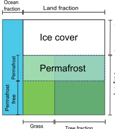
Ice cover
Land fraction
Ocean fraction
Grass
fraction Tree fraction
Ice cover
e
d
Ice free
P
er
m
af
ro
st
P
er
m
a
fr
o
st
f
ree
Permafrost
Figure 1. A CLIMBER-2P grid cell showing the distribution of dif-ferent cell cover types.
the atmosphere was seen from ice core data. Soil carbon has aδ13C signature depleted by around 18 ‰ compared to the atmosphere (Maslin and Thomas, 2003); a release of carbon from thawing permafrost soils is a possible explanation for theδ13CO2record.
In this study, we aim to develop a permafrost-carbon model for long-term paleoclimate studies. We present the de-velopment of the permafrost-carbon model and validate it with present-day ground measurement data for soil carbon concentrations in high northern latitude soils.
2 Model development
2.1 CLIMBER-2 standard model
The CLIMBER-2 model (Petoukhov et al., 2000; Ganopol-ski et al., 2001) consists of a statistical–dynamical atmo-sphere, a three-basin averaged dynamical ocean model with 21 vertical uneven layers and a dynamic global vegetation model, VECODE (Brovkin et al., 1997). The model version we use is as Bouttes et al. (2012) and Brovkin et al. (2007). The model can simulate around 20 kyr in 10 h (on a 2.5 GHz processor) and so is particularly suited to paleoclimate and long-timescale fully coupled modelling studies. The ver-sion of CLIMBER-2 we use (Bouttes et al., 2009, 2012) is equipped with a carbon-13 tracer, ice sheets and deep sea sediments (allowing the representation of carbonate com-pensation) in the ocean (Brovkin et al., 2007) as well as ocean biogeochemistry. The ice sheets are determined by scaling ice sheets’ size between the LGM condition from Peltier (2004) and the Pre-Industrial (PI) ice sheet using the sea level record to determine land ice volume (Bouttes et al.,
2012). The dynamic vegetation model has two plant func-tional types (PFTs), trees and grass, plus bare ground as a dummy type. It has two soil pools, “fast” and “slow”, rep-resenting litter and humus respectively. Soils have no depth, and are only represented as carbon pools. The carbon pools of the terrestrial vegetation model are recalculated once ev-ery year. The grid cell size of the atmospheric and land surface models is approximately 51◦ longitude (360/7 de-grees) by 10◦latitude. Given the long-timescale applications of the CLIMBER-2 model and the very large grid size for both atmosphere and land, none of the existing approaches of modelling permafrost carbon are suitable. Thermal diffusion-based physical models would produce results with unaccept-able uncertainties (error bounds) compounding over long timescales. To create the permafrost model for CLIMBER-2, the driving mechanism creating high soil carbon concentra-tions is a reduced soil decomposition rate in the presence of permafrost, identified by Zimov et al. (2009) as the primary driver in soil carbon accumulation for these soils.
2.2 Permafrost-carbon mechanism
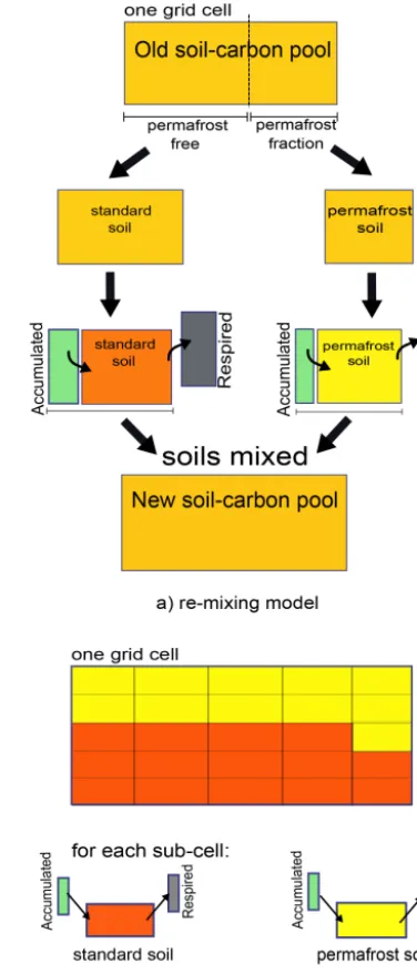
CLIMBER-2 grid cells for the land surface model are very large. Two options are available to diagnose permafrost loca-tion: either by creating a sub-grid within the land grid or by diagnosing a fraction of each grid cell as permafrost, which is the approach followed here. Conceptually the sub-grid model represents keeping permafrost carbon separate from other soil carbon, and the remixing model represents mixing all soil carbon in a grid cell. Figure 1 shows a schematic repre-sentation of a CLIMBER-2 grid cell, and how the permafrost fraction of the land is defined relative to other cell parameters when permafrost is diagnosed as a fraction of each cell. For the carbon cycle the calculations of carbon fluxes between at-mosphere and land grid cells are for the cell mean. Each grid cell contains cell-wide soil carbon pools (fast soil or slow soil, per plant functional type), so to account for permafrost soils either a new permafrost-soil pool needs to be created for each grid cell, or permafrost soils can be mixed back into the standard soil pools at every time-step (Fig. 2a). If the land grid is downscaled a third option is available, where each sub-grid cell maintains an individual soil carbon pool (Fig. 2b). This, however, requires an increase in computa-tional time which slows down the run speed of the model.
The soil carbon in CLIMBER-2 is built from vegetation mortality and soil carbon decomposition is dependent on surface air temperature, the total amount of carbon in the pool and the source of carbon (i.e. trees or grass). Equa-tion (1) shows how carbon content of each pool is calcu-lated in CLIMBER-2. The pool is denoted by Ci, where pool
The equations (Eq. 1) are numerically solved in the model with a time-step of one year.
dCp1 dt =k
p 1N−m
p 1C
p 1
dCp2
dt =(1−k p 1)N−m
p 1C
p 2
dCp3 dt =k
p 2m
p 1+k
p 3m
p 2C
p 2−m
p 3C
p 3
dCp4 dt =k
p 4m
p 2C
P
2 +k p 5m
p 3C
p 3−m
p 4C
p
4, (1)
where C is the carbon content in the pool (kgC m−2);kis al-location factors (0< ki <1);N is net primary productivity (NPP; kgC m−2yr−1);miis decomposition rates for the
car-bon in each pool (yr−1); p is the plant functional type (trees or grass).
The residence time of carbon in soil pools is 1/m; we call thisτ. For residence times corresponding to decomposition ratesm3andm4,τ is:
τi=npi ·e(−ps5(Tmat−Tref)), (2)
wherei is the soil pool,nis a multiplier dependent on the pool type, ps5 is a constant,=0.04,Tmatis mean annual tem-perature at the surface–air interface, ◦C,Trefis a reference soil temperature, fixed in CLIMBER-2 at 5◦C.
The value of n is dependent on the soil carbon type, being 900 for all slow soils, 16 for fast tree PFT soil and 40 for fast grass PFT soil. The decomposition rates for organic residue in the soils are most strongly based on soil microbial activity and the relative amount of lignin in the residues (Aleksan-drova, 1970; Brovkin et al., 1997). Increasing the residence time of carbon in permafrost-affected soils reduces the de-composition rates and results in higher soil carbon concen-trations. We modify the residence time,τ3,4, in the presence of permafrost using:
τ(permai)=τi(aFsc+b), (3)
whereaandbare tuneable dimensionless constants andFsc is frost index, a value between 0 and 1, which is a measure of the balance between cold and warm days in a year, and is shown in Eq. (4) where DDF is degree-days below 0◦C and DDT is degree-days above 0◦C in a year for daily
av-erage surface air temperature (Nelson and Outcalt, 1987). DDF and DDT have units of◦C days yr−1. Snow cover acts to insulate the ground against the coldest winter temperatures and reduces permafrost extent (Zhang, 2005; Gouttevin et al., 2012). The subscript sc in Eqs. (3) and (4) indicates that these values are corrected for snow cover and represent the ground–snow interface conditions, not the snow surface–air interface conditions.
Fsc=
DDF(sc1/2) DDF(sc1/2)+DDT(1/2)
(4)
Figure 2. Schematic of a CLIMBER-2P grid cell showing how car-bon is accumulated at each time-step. Remixing model (a) separates grid cell into permafrost or non-permafrost, calculates the change in carbon pool and remixing all carbon in the cell back together. Sub-grid model (b) separates the Sub-grid cell into 25 sub-Sub-grid cells, calcu-lates change in carbon pool in each individually and does not remix any carbon between sub-grid cells.
cold-0 0.1 0.2 0.3 0.4 0.5 0.6 0.7 0.8 0.9 1 0
0.1 0.2 0.3 0.4 0.5 0.6 0.7 0.8 0.9 1
Re-mixing Sub-grid
Permafrost fraction
Re
la
tive soi
l car
bon
co
ntent
Figure 3. Comparison of sub-grid to remixing approach for relative soil carbon contents of a grid cell for increasing permafrost frac-tion. The variables of mean annual temperature and frost index vary with permafrost fraction according to data relationships upscaled to CLIMBER-2 grid relationships (see Appendix A and Fig. A2).
ness in a year). Thisτpermai(Eq. 3) is only applied to the soils
that are diagnosed as permafrost. The remainder of the car-bon dynamics in land carcar-bon pools was unaltered from the standard model.
2.3 1-D model
We test a one-dimensional model to compare the effect the different assumptions made for the model design. The total carbon stock in a grid cell using each method (sub-grid and remixing) was compared for equilibrium soil carbon content by running the 1-D model for 100 000 simulation years. The carbon input from vegetation mortality is the same for the remixing and the sub-grid model, as is rainfall. The vari-ables of permafrost fraction, mean annual air–surface inter-face temperature (MAT) and frost index are varied one at a time to compare the model outputs. The constants a andb for Eq. (3) were set to 20 for Soilfastand 2 for Soilsslow(soa andbhave matching values) for the permafrost soils, and as the standard model for the non-permafrost soils. These val-ues fora andbwere chosen to compare the performance of the two methods, not for accurate soil carbon concentrations. They result in total carbon in the Soilfastand the Soilslow car-bon pools being approximately equal, which studies suggest is appropriate (Harden et al., 2012; Zimov et al., 2009).
Figure 3 shows the output for carbon content along a per-mafrost gradient, taking account of the relationship between permafrost fraction, frost index and mean annual tempera-ture. More detail on this figure is available in Appendix A. The relationship between permafrost fraction and frost index is defined as that determined in this study for the CLIMBER-2 model in Sect. 3.CLIMBER-2. As shown in Eq. (1), NPP exerts a con-trol on soil carbon content via input from plant material, al-though note that Fig. 3 shows model output for fixed NPP. For both approaches, carbon content increases non-linearly
Figure 4. Comparison of NPP, which has a control on carbon input to soils, for MODIS data set (top, mean 2000–2005) and CLIMBER-2 model for PI(eq) (modelled year 1950) plotted on the same scale (gC m−2yr−1). MODIS data upscaled to CLIMBER-2 grid scale are shown against equivalent points for CLIMBER-CLIMBER-2 NPP.
along the permafrost gradient (increasing permafrost frac-tion of the grid cell). The remixing model shows stronger non-linear behaviour than the sub-grid model.
2.4 CLIMBER-2 modelled NPP
Figure 5. Comparison of NPP, which has a control on carbon in-put to soils, for LPX model (top, courtesy of M. Martin-Calvo, av-erage of an ensemble model output) and CLIMBER-2 model for LGM(eq) (at 21 kyr BP) plotted on the same scale (gC m−2yr−1), and the same scale as Fig. 4. LPX output upscaled to CLIMBER-2 grid and plotted against equivalent CLIMBER-2 NPP is shown also.
via NPP in colder climates. Figure 4 shows the CLIMBER-2 modelled NPP and the MODIS 2000–2005 mean NPP prod-uct (Zhao et al., 2011) for the present day (PI, pre-industrial for CLIMBER output). The CLIMBER-2 vegetation model shows NPP patterns similar to the MODIS data set. The
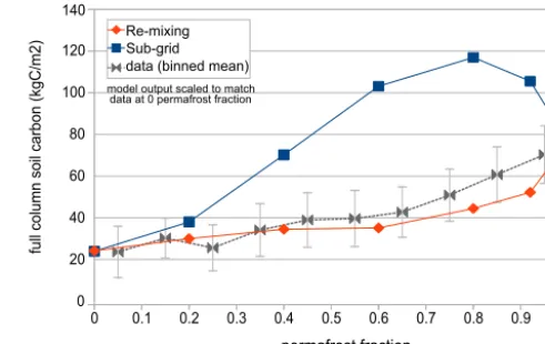
bo-0 0.1 0.2 0.3 0.4 0.5 0.6 0.7 0.8 0.9 1 0
20 40 60 80 100 120 140
model output scaled to match data at 0 permafrost fraction
Re-mixing Sub-grid data (binned mean)
permafrost fraction
full
co
lu
m
n soi
l car
bon
(
kgC
/m
2)
Figure 6. Modelled output for 1-D models along a permafrost gra-dient, with correction for NPP and initial value (at 0 % permafrost). Overlaid on 1◦data for SOCC binned into 0.1 permafrost fraction mean values±1 sigma (Hugelius et al., 2013), permafrost fraction is calculated using relationship identified in Sect. 3.2.
0 0.2 0.4 0.6 0.8 1 0 0.5 1 1.5 2 2.5 3
ALT mean value Linear regression ALT
Frost index mean
A ct ive la yer t h ickn ess ( A LT ) d ata up scal ed to CL IM B E R -2 gr id ( m )
R2 = 0.87
Figure 7. Measurement data for active layer thickness (CALM net-work, Brown et al., 2003) and frost index (Zhang, 1998) upscaled to the CLIMBER-2 grid scale, showing the distinct relationship of reducing active layer with increasing frost index at this scale. Note that permafrost fraction is calculated from frost index in our model (see Sect. 3.2).
When the soil carbon content shown in Fig. 3 is adjusted to compensate for the reduction in NPP along a permafrost gradient and for the 0 % permafrost SOCC data value (by multiplying relative value by 350), the resultant outputs are shown in Fig. 6 (more details are available in Appendix A). Now the remixing model shows a slight increase in total car-bon along a permafrost gradient, where the sub-grid model shows a peak value at around 80 % permafrost coverage. Fig-ure 6 shows a comparison between these 1-D model outputs and data for SOCC. The unadjusted data are for the top 1 m of soils, whereas model output represents the full soil col-umn. As in Sect. 4.4, the model–data comparison is carried out by assuming that 40 % of total soil carbon is located in the top 1 m for permafrost soils (and is fully described in Ap-pendix A). From this comparison, the change in SOCC along a permafrost gradient is relatively small, due to the com-bined effects of reducing soil decomposition rate and reduc-ing NPP. Here, the remixreduc-ing model represents these changes quite well. It may be possible to improve the performance of the sub-grid model by, for example, downscaling the climate variables also. However, this would represent a more signif-icant change of the land biosphere model in CLIMBER-2, and increase the complexity and therefore reduce the compu-tational efficiency of the model.
For the remixing model: at each time-step a proportion of carbon that is accumulated in the permafrost part is then sent back to decompose as standard soil. This occurs because the high-carbon permafrost soil is mixed with the lower carbon standard soil in a grid cell at each time-step. This can be seen as similar to that which occurs in the active layer. The active layer is the top layer of the soil that thaws in warm months and freezes in cold months. In warm months the carbon in this thawed layer is available to be decomposed at “standard”
0.52 0.53 0.54 0.55 0.56 0.57 0.58 0.59 0.6 0.61
10 12 14 16 18 20 22
Frost-index derived area High data estimate Mean data estimate Low data estimate
Frost-Index cut off value
La
nd
a
rea
(x 10
6 km
2)
Figure 8. Total land area with a frost index higher (colder) than the xaxis cut-off value, for frost-index data from Zhang (1998) (NSIDC). Horizontal lines show the Zhang et al. (2000) data es-timates for area of land underlain by permafrost.
soils rates, determined by local temperature. In the remixing model, the relative proportion of the permafrost soil carbon that is sent to decompose as standard soil carbon reduces along a permafrost gradient. This reduction can be seen as mimicking the characteristic of a reducing active layer thick-ness along a permafrost gradient, which is shown in Fig. 7 for active layer thickness data upscaled to the CLIMBER-2 grid size. Here active layer thickness mean is shown plot-ted against mean frost index (and permafrost fraction is di-rectly calculated from frost index in CLIMBER-2). It must be noted that on smaller spatial scales the relationship between the mean active layer thickness and the extent of permafrost in a location may be less clear. The local conditions deter-mine both permafrost extent and active layer thickness. Our treatment for permafrost relies entirely on the relationships between climate characteristics and soil carbon contents on the CLIMBER-2 grid scale.
3 CLIMBER-2 permafrost-carbon model
Figure 9. Map of land with frost index greater than 0.57 (frost in-dex predicted permafrost) shown in blue with southern limit of per-mafrost boundaries for the present day defined by IPA overlaid. Black line: continuous permafrost, pink line: discontinuous per-mafrost, green line: sporadic permafrost. Grey dotted lines are the CLIMBER-2 grid.
3.1 Simulated climates to tune the permafrost-carbon model
Three simulated climates were used to tune and validate the permafrost-carbon model: an LGM equilibrium climate, LGM(eq); a PI equilibrium climate, PI(eq); and a PI transient climate, PI(tr) obtained at the end of a transient deglaciation from the LGM climate. These three climates allow the total soil carbon to be tuned to the estimates of Ciais et al. (2012) for the LGM and PI climate conditions; these are described in Table 1.
3.2 Calculating permafrost extent
In order to obtain a relationship between calculated frost index and the permafrost fraction of a grid cell, measure-ment and ground data for frost index and permafrost location were used. For present-day mean daily surface air temper-atures, the freeze and thaw indices values on a 0.5◦ global
grid were obtained from the National Snow and Ice Data Centre (NSIDC) database (Zhang, 1998). Using these val-ues for freeze and thaw index, a global frost-index data set on a 0.5◦grid scale was created using Eq. (4). The present-day estimates of land area underlain by permafrost are pro-vided by Zhang et al. (2000), using the definition of zones: “continuous” as 90–100 % underlain by permafrost,
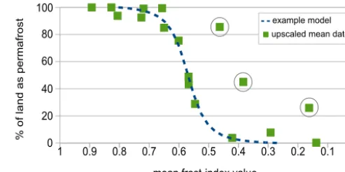
“discon-0 0.1 0.2 0.3 0.4 0.5 0.6 0.7 0.8 0.9 1 0 20 40 60 80 100
example model upscaled mean data
mean frost-index value
%
o
f la
nd as pe
rm
afr
os
t
Figure 10. Frost-index-predicted permafrost fraction of land from Fig. 8 upscaled to the CLIMBER-2 grid and plotted against mean frost index for the same CLIMBER-2 grid cell. Circled points are where the total fraction of land vs. ocean in the grid cell is small (land is less than 25 % of the grid cell) and ocean temperatures pull frost index lower (warmer). The dashed line is a representative re-lationship between frost index and permafrost land fraction.
tinuous” as 50–90 %, “sporadic” as 10–50 % and “isolated” as less than 10 %. Zhang et al. (2000) used these zonations to provide area estimates of the total land area underlain by permafrost. Summing the total land area that has a frost index higher than a particular value and comparing this to the Zhang et al. (2000) estimate can identify the appropriate boundary between permafrost and non-permafrost soils. Fig-ure 8 shows the Zhang et al. (2000) permafrost areas for the high, medium and low ranges defined by the high, medium and low % estimates of permafrost zones marked as hori-zontal lines. The land area indicated by green squares is the total land surface in the northern hemisphere that has a frost-index value higher (where higher indicates a colder climate) than the cut-off value shown on thex axis. Here the frost-index cut-off value of 0.57 shows good agreement with the medium (mean) estimate of the Zhang et al. (2000) total area of land underlain by permafrost.
3.3 Geographic permafrost distribution for the present-day
Figure 9 shows, coloured in blue, the land grid cells with a frost-index higher than 0.57 for 0.5◦ grid, with the north located at the centre of the map. Overlaid on this map area are the limits of the permafrost zones defined by the Interna-tional Permafrost Association (IPA) (Jones et al., 2009). The frost-index value cut-off at 0.57 results in a southern limit of permafrost that represents approximately the middle of the discontinuous zone with some areas showing better agree-ment than others.
Table 1. Simulated climates used in this study.
Date Event
LGM (equilibrium) Obtained after an 80 kyr spin-up with glacial CO2levels of 190 ppmv, reduced ocean volume, LGM ice sheets, LGM insolation, LGM runoff. Carbonate compensation in the ocean (Brovkin et al., 2002). Sea-level effects on coast lines are not included; land area is as PI (equilibrium). The continental shelves exposed at LGM are not accounted for in this model set-up because the fate of any carbon that may have accumulated on these shelves is not well constrained. The long time of spin-up, 80 kyr, is required to allow the soil carbon pools to equilibrate.
PI (equilibrium) Obtained after 40 kyr spin-up with pre-industrial CO2levels of 280 ppmv, present-day ocean volume, present-day ice sheets, insolation, and land run-off. The 40 kyr spin-up time allows soil carbon pools to equilibrate.
PI (transient) End of a 21 kyr simulation of a transient deglaciation that has the LGM equilibrium climate as a start point at 21 kyr BP. The PI (transient) is the climate at 0 yr BP. The transient deglaciation has evolving ice sheets scaled to sea-level, increasing ocean volume, insolation changes (seasonality), carbonate compensation and LGM runoff. This transient PI climate is required to account for the long time to equilibrium of the permafrost-affected soil carbon pools. In order to compare model output with ground-data the PI(transient) provides a more realistic model output.
Circled points in Fig. 9 are where the grid cell has a large fraction of ocean (more than 75 %), and the milder ocean temperatures in winter reduce the mean frost-index value of the whole grid cell. The dashed line shows a well-defined sigmoid function that relates frost index to permafrost per-centage of the land. We employ this relationship to predict permafrost area in CLIMBER-2, as the frost index can be calculated within the model from modelled daily tempera-tures. Permafrost fraction is thus modelled as:
Plandfraction=A(0.976+ β p
(1+β2))−0.015, (5) where A and β are defined in Table 2 and the model de-scribed in Sect. 3.5. Frost index is calculated from modelled daily surface temperatures and corrected for snow cover. The snow correction in our model is achieved using a simple lin-ear correction of surface–air temperature, using snow thick-ness to estimate the snow–ground interface temperature. This correction is based on data from Taras et al. (2002). The snow correction performs reasonably well in CLIMBER-2 compared to measurement data from Morse and Burn (2010) and Zhang (2005). This is because the large grid-cell size results in non-extreme snow depths and air surface tempera-tures. The snow correction is described in Appendix B. Equa-tion (6) shows this linear model for snow correcEqua-tion, which is only applied for daily mean surface air temperatures lower than−6◦C. This snow–ground interface temperature is used to calculate the freeze index (DDFsc)in Eq. (4).
Tg.i−Tsurf−
(Tsurf+6)·SD
100 , (6)
whereTg.iis ground interface temperature (◦C),Tsurfis sur-face air temperature (◦C) and SD is snow depth (cm). Overall the effect of the snow correction within the model produced
Table 2. Permafrost area model settings for Eq. (5).
A β
HIGH 0.58 22(Fsc−0.58) MED 0.555 21(Fsc−0.59) LOW-MED 0.54 20.5(Fsc−0.595) LOW 0.53 20(Fsc−0.6)
a maximum decrease in permafrost area of 8 % (compared to the uncorrected version) in the most affected grid cell for the PI(eq) simulation and is therefore significant.
3.4 Permafrost extent tuning
0 0.1 0.2 0.3 0.4 0.5 0.6 0.7 0.8 0.9 1 0 0.2 0.4 0.6 0.8 1 HIGH area MED area LOW-MED area LOW area Frost index P er m a fr o st f ra ct ion
Figure 11. CLIMBER-2P model for permafrost fraction of the land in a grid cell from frost index (snow corrected). Range of areas is within the range of estimates for present-day land area underlain by permafrost by Zhang et al. (2000). Permafrost fraction is limited between 0 and 1. Zhang estimate for total permafrost area is 12.21 to 16.98×10⁶km2. Listed from HIGH to LOW, model output is 16.35, 14.87, 14.00 and 13.21×10⁶km2.
3.5 Tuning the soil carbon model
Soil carbon content is controlled by the balance between soil carbon uptake and soil carbon decomposition. There are four soil carbon pools in CLIMBER-2: Soilfast: trees derived and grass derived; Soilslow: trees derived and grass derived (Eq. 1). Soilfast have shorter carbon residence times than Soilslow, so soil decays more quickly in Soilfast pools. The tunable constantsaandb (Eq. 3) are independently applied for Soilfast and Soilslow, so carbon can be placed relatively more in the Soilfast(Soilslow)pool as required in model tun-ing. Carbon is lost from permafrost soils as the permafrost fraction of a grid cell reduces. If there is relatively more (less) carbon in the Soilfast pool, this results in carbon that decays more quickly (more slowly) when the permafrost thaws.
At LGM, the area of permafrost on land was larger than today (Vandenberghe et al., 2012), but not much informa-tion on soil carbon has been conserved, especially if it has long since decayed as a result of permafrost degradation dur-ing the last termination. To constrain the total carbon con-tent in permafrost soils we use the estimates of Ciais et al. (2012); for total land carbon these are 3640±400 GtC at LGM and 3970±325 GtC at PI, with a total change of
+330 GtC between LGM and PI. The standard CLIMBER-2 model predicts total land carbon stocks of 1480 GtC at LGM and 2480 GtC at PI, showing good agreement with the active-land-carbon estimates of Ciais et al. (2012) (of 1340±500 GtC LGM and 2370±125 GtC PI). Any “new” soil carbon is created via the permafrost-carbon mechanism and is assumed to be equivalent to the inert land carbon pool estimates of Ciais et al. (2012). However, the dynamic be-haviour of permafrost-carbon in changing climates is not well constrained and it is for this reason that a set of four dynamic settings were sought. Here the “speed” of the
dy-Table 3. Selected settings for permafrost decomposition function, where subscript indicates the soil pool. Permafrost area model is LOW-MEDIUM for all.
Constants’ settings for Eq. (3)
Dynamic settings afast bfast aslow bslow
Slow 10 10 10 10
Medium 20 40 1 3
Fast 60 50 0 1
Xfast 60 80 0.1 0.1
namic setting is determined by the ratio of total Soilfast pool to Soilslow pool carbon (fp/sp), with the “slow” dynamic being fp/sp <0.5, “medium” being fp/sp 0.5 to 1, “fast” being fp/sp 1 to 1.5 and “extra-fast” being fp/sp>1.5 for the PI-equilibrium simulation. The variables “a” and “b” shown in Eq. (3) were set and each setting used to run a PI(equilibrium), LGM(equilibrium) and PI(transient) simu-lation to identify the settings that resulted in total land carbon pools in agreement with the Ciais et al. (2012) estimates.
The LGM is conventionally defined as being the period around 21 kyr BP, when large parts of north America were underneath the Laurentide ice sheet. According to their time-to-equilibrium (the slow carbon accumulation rate), soils in this location now free of ice may not yet have reached equilibrium. Furthermore, climate has changed significantly since the LGM so permafrost soils anywhere may not be cur-rently in equilibrium (Rodionov et al., 2007), again due to their slow carbon accumulation rates. Due to this the PI(tr) simulation model output for total land carbon was used to tune the total land carbon stocks, as it includes a receding Laurentide ice sheet. At LGM, ice sheets were at maximum extent, so the problem of land being newly exposed does not occur in the model. For this reason, the LGM(eq) simulation is used to tune total land carbon for the LGM.
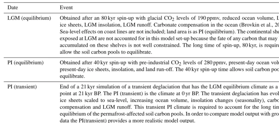
Details of the tuning for total land carbon stocks are avail-able in Appendix C. It was found that only one permafrost area setting, the LOW-MEDIUM area, provided an accept-able range of dynamic settings, as defined by the ratio of fast to slow soil carbon. The four selected dynamics settings are shown in more detail in Fig. 12 for total land carbon stock, atmospheric CO2and ratio of fast to slow soil carbon pool. Theaandbvalues for these settings are shown in Table 3.
pre-Figure 12. Chosen dynamic settings for the range of permafrost-carbon dynamics. Left: total land carbon with Ciais et al. (2012) estimates as dashed lines. Middle: atmospheric CO2(ppm). Right: ratio of all fast to all slow soil pools, indicating the speed of response of the soil carbon to changing climate.
slow medium fast xfast no permafrost
total la
nd
ca
rbo
n (
G
tC)
simulation year
P
er
m
a
fr
o
st
swi
tch
-off
Figure 13. Total land carbon (GtC) for the PI(eq) simulation fol-lowed by a permafrost switch-off at 40 k simulation years repre-senting a complete and immediate permafrost thaw, demonstrating the different dynamic behaviour of each dynamic setting.
viously held in permafrost soils is quickly released to the at-mosphere, at a rate dependent on the dynamic setting. The xfast setting entails releasing all excess carbon within hun-dreds of years and the slow setting around 8000 years after total permafrost disappearance. Currently, the most appropri-ate carbon dynamic setting is unconstrained by measurement data. It is for this reason that the permafrost-carbon dynam-ics settings cover a large range. They are intended to be used in transient model simulations to better constrain permafrost-carbon dynamics in changing climate. It should be noted that the PI(eq) simulation was not used to tune the model, i.e. was not used to compare model output to Ciais et al. (2012) PI to-tal land carbon stocks. Figure 13 demonstrates only the range of dynamic response for all four settings. This PI(eq) simu-lation also demonstrates the difference between transient vs. equilibrium PI simulations. The slow dynamic equilibrates (after more than 40 kyr) at far higher total carbon stocks than the xfast dynamic, but for the PI(tr) simulation these two set-tings show very similar total land carbon stocks (we selected them for this behaviour).
4 Model performance
Hereafter, “CLIMBER-2P” denotes the model in which the permafrost-carbon mechanism operates fully coupled within the dynamic vegetation model.
4.1 Permafrost areal coverage and spatial distribution
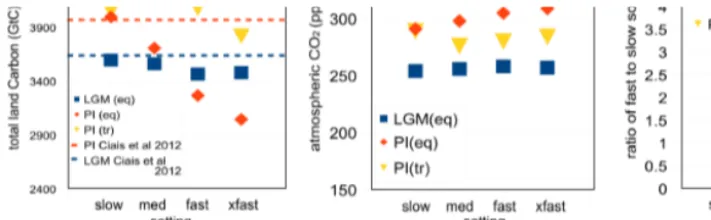
Figure 14a shows the spatial pattern of permafrost as pre-dicted in CLIMBER-2P with the snow correction included for the LOW-MEDIUM area setting. The modelled PI(tr) permafrost extent estimates fairly well the location of the present-day southern boundary of the discontinuous mafrost zone (Jones et al., 2009), with overestimate of per-mafrost extent in the western Siberian grid cell, and under-estimate over the Himalayan plateau. Total permafrost area extent is shown in Table 4.
Comparing this to performance of other models (Lev-avasseur et al., 2011), the PI(eq) total permafrost area is closer to Zhang et al. (2000) estimates, but it must be kept in mind that for CLIMBER-2P the area was tuned to be in agreement with a mean estimate from Zhang et al. (2000). The PI(tr) total permafrost area is higher by around 4×
106km2 compared to the PI(eq). This is due to the North Pacific region being colder in PI(tr) than that of the PI(eq) simulation, and may be related to the land run-off, which is kept at LGM settings for the transient simulations. For the LGM period, the best PMIP2 model in the Levavasseur study (interpolated case) underestimated total permafrost area by 22 % with respect to data estimates (of 33.8×10⁶km2), and the “worst” model by 53 %, with an all-model-median value of 47 % underestimate. The LOW-MEDIUM CLIMBER-2P setting gives an LGM total permafrost area underestimate of around 40 %, slightly better than the median for PMIP2 mod-els’ permafrost area.
Table 4. Modelled permafrost-affected land area and data-based estimates.
Permafrost area (×106km2)
(land underlain by permafrost)
Permafrost model area setting
Pre-industrial cli-mate (equilibrium)
Pre-industrial climate (transient)
Glacial climate
LOW-MEDIUM 14.0 18.4 20.7
Data estimate 12.21 to 16.98 (Zhang et al., 2000) 33.8 (Levavasseur et al., 2011) 40 (Vandenberghe et al., 2012)
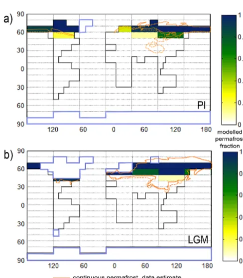
Figure 14. Modelled permafrost area for (a): PI(tr) simulation, (b) LGM(eq) simulation for LOW-MEDIUM permafrost area. Over-laid in orange are data estimates from Circumpolar Atlas (Jones et al., 2009) for the present day, Vandenberghe et al. (2008) for LGM Eurasia, French and Millar (2013) for LGM N. America.
and other exposed coastlines in the northern polar region are not included in the CLIMBER-2P permafrost area esti-mate. These coastal shelves cover an estimated area of 5 to 7×10⁶km2. Another area that is not diagnosed as permafrost in CLIMBER-2P is the Tibetan plateau, which would be an additional estimated 6×10⁶km2. If these two regions were added (totalling around 12×106km2)to the LGM area es-timate it would bring the modelled permafrost area (then to-talling around 33×106km2)much closer to the data esti-mate as reported in the Levavasseur et al. (2011) study. The permafrost extent model is dependent on the CLIMBER-2P modelled climate. The very large grid cell size of CLIMBER-2P means that modelled mountainous regions such as the
0 5000 10000 15000 20000 25000 30000 35000 40000 0
20 40 60 80 100 120 140 160
north Canada
slow med fast xfast
simulation years
soi
l car
b
on
co
nten
t,
kg
C/m
2 Extra cold (Zimov et
al 2009)
ES
simulation years
0 5000 10000 15000 20000 25000 30000 35000 40000 45000
0 50 100 150 200 250
north west Siberia
slow med fast xfast
soi
l car
b
on
co
nten
t,
kg
C/m
2
Extra cold (Zimov et al 2009) Ayach-Yakha
(Wania et al 2009)
ES
Figure 15. Modelled PI(eq) simulation output for total soil column carbon content for two grid cells. ES is equilibrium state (>50 kyr).
Tibetan plateau are problematic, resulting in a possible too-warm climate (compared to the real world) in this region. 4.2 Soil carbon dynamics
that 200 kg m−2 soil carbon content can be reached within 10 kyr in the top layer of the soil and 150 kg m−2 for the full soil column taking longer than∼50 kyr to reach equilib-rium. The N. Canada (Fig. 15) location takes a longer time to reach equilibrium than soils in the NW Siberia grid cell. NPP in the N Canada grid cell is less than one third of that for the NW Siberia grid cell. Due to the lower soil carbon input there is a lower range in the output between the dif-ferent carbon dynamic settings for the N Canada grid cell. Northern Canada was underneath the Laurentide ice sheet at LGM. Since the demise of the Laurentide ice sheet around 13 kyr ago (Denton et al., 2010) there has not been enough time for these soils to equilibrate, which takes longer than 40 kyr according to our model. As well as this, this region has very high water contents (and islands) that are not rep-resented in CLIMBER-2P, which may modify soil carbon concentrations. Although we do not account for water con-tent, we can take account of the demise of the Laurentide ice sheet and the time that these soils have had to accumulate carbon. The PI climate condition and soil carbon content that we applied to tune and validate the model are the PI(tr), the transient simulation, which includes ice sheet evolution. 4.3 Soil carbon stocks
The total land carbon stocks were tuned using data from Ciais et al. (2012). An assumption made in this study is that all “ex-tra” soil carbon, relative to the standard model, in the Arctic region is located in permafrost soils and only by the mecha-nism of increased soil carbon residence time in frozen soils. Table 5 shows the Ciais et al. (2012) land carbon pools values that have been used to tune this model. The standard model total land carbon (tlc) values are similar to the active land car-bon stocks, with PI tlc at 2199 GtC and LGM tlc at 1480 GtC (shown in Table 7).
The soil types that are found in the continuous and discon-tinuous permafrost zone are the Cryosols (circumpolar atlas) or Gelisols (soil taxonomy). Within this group are subgroups: Turbels, which are subject to cryoturbation and characterise the continuous permafrost zone; Orthels, which are less af-fected by cryoturbation and are related to discontinuous per-mafrost; and Histels, which relate to peat growth (histosols) and have permafrost at less than 2 m depth. Histels are not directly represented in the simplified model, as they are dom-inated by peat growth (Sphagnum), a distinct PFT not repre-sented in CLIMBER-2P.
The Tarnocai et al. (2009) SOCC estimates for the present day for relevant soils are shown in Table 6. Summing “All soils” with loess soils and Deltaic deposits gives the 1672 GtC estimated total SOCC for the permafrost region. The extra land carbon stocks created in our model in per-mafrost soils range between 1620 to 2226 GtC (Table 8) com-pared to Tarnocai et al. (2009) at 1672 GtC and to Ciais et al. (2012) at 1600±300 GtC for inert land carbon for the present day. For the LGM climate, the model shows a range
of 1987 to 2117 GtC for extra soil carbon compared to the Ciais estimate of 2300±300 GtC for inert land carbon. The “medium” dynamic setting shows total land carbon stocks in the present day outside the range estimated by Ciais et al. (2012), However, during tuning (see Appendix C) this overestimate could not be improved upon.
4.4 Soil carbon contents validation
The carbon content of Orthels and Turbels decreases with depth, but high carbon contents are still found at depths of 3 m and more (Tarnocai et al., 2009). For Orthels (with al-luvium), around 80 % of their carbon content was found in the top 200 cm, and for Turbels 38 % of carbon content was found in the top 100 cm. Based on these values, to compare the CLIMBER-2P output with ground spatial data, it is as-sumed that 40 % of the modelled total soil-column carbon is located in the top 100 cm for all permafrost-affected soils.
Soil carbon data from Hugelius et al. (2013) were used to compare against the CLIMBER-2P output. The Orthels and Turbels dominate the continuous and coldest permafrost ar-eas, with Histels and other soils becoming more dominant to-wards the southern parts of the permafrost region. As no peat-lands or wetpeat-lands are represented in our simplified model, only Orthel and Turbel soils were used as comparison points for SOCC. SOCC data from Hugelius et al. (2013), for grid cells with 50 % or more Orthel and Turbel soils, were up-scaled to the CLIMBER-2P grid. These mean SOCC data values for the top 1 m of soil were plotted against CLIMBER-2P model output for matching grid cells; this is shown in Fig. 16. Also shown in Fig. 16 is the standard model output, which has no permafrost mechanism. Two grid cells show very much higher SOCC than data suggest, with around a 3-fold overestimate, and are located in Siberia. All other grid cells are within a range of±80 %, heavily dependent on the soil carbon dynamic setting. The standard model shows pro-gressively worse performance as mean SOCC increases in the data. The permafrost model shows an increasing SOCC trend more similar to data. The spatial location of SOCC can be compared to data using Fig. 17. The two grid cells with very high SOCC compared to data are central and eastern Siberia. These grid cells are both 100 % permafrost and have had a total of 101 kyr (80 k for LGM(eq) plus 21 k to PI(tr)) to accumulate carbon. This is in contrast to the North Ameri-can continent grid cells, which were underneath the ice sheet until the deglaciation so have had less time to accumulate carbon.
Table 5. Total land carbon stock estimates from Ciais et al. (2012).
Period Total land carbon (GtC) Active land carbon (GtC) Inert land carbon (GtC)
Present day 3970±325 2370±125 1600±300
LGM 3640±400 1340±500 2300±300
Table 6. Permafrost region soil carbon stock estimates from Tarnocai et al. (2009).
Soil type Depth Soil carbon (GtC)
Gelisols To 1 m Turbels 211.9
Orthels 51.3
Histels 88.0
All 351.5
To 3 m Turbels 581.3
Orthels 53.0
Histels 183.7
All 818.0
All soils To 1 m 495.8
To 3 m 1024.0
Pleistocene loess >3 m 407
Deltaic >3 m 241
an estimated 390 GtC (Tarnocai et al., 2009), are not repre-sented in our model. If these were modelled they should in-crease SOCC in model output in the more southern part of the permafrost region, and parts of Canada. Large river deltas, which contain deltaic deposits of 241 GtC (Tarnocai et al., 2009), are also not represented in our model. One example of this is the Ob River and Gulf of Ob, located in western Siberia, which, combined with dominance of Histels in this region (Hugelius et al., 2013), cause a high SOCC in data. The model does not represent well the boreal forest belt (see Fig. 4), which is also located in the southern region of the permafrost zone. This results in carbon input to soils in this region being underestimated in our model.
Figure 18 shows the model outputs for the LGM cli-mate. No soil carbon is present underneath ice sheets and the highest carbon concentrations are seen in present-day south-eastern Russia and Mongolia, with quite high soil carbon concentrations in present-day northern Europe and north-western Russia. Comparing this output to the permafrost ex-tent model (Fig. 14), the SOCC is likely located too far north for the same reasons as the PI(tr) SOCC but also because per-mafrost extent is underestimated for the LGM(eq) climate. The northern China region, according to data, was continu-ous permafrost at LGM, as was the southwest Russia region. These regions would have higher SOCC in model output if the modelled permafrost area were closer to data estimates. The same would be true of the Siberian shelf. This means that the extra soil carbon tuned to the Ciais et al. (2012) estimate
Figure 16. Modelled SOCC (kgC m−2) for the top 1 m plot-ted against SOCC data for the top 1 m of soil upscaled to the CLIMBER-2 grid scale. Circles are for the permafrost-carbon model (CLIMBER-2P); triangles are for the standard model (CLIMBER-2). Dotted line shows the 1:1 position. Points are SOCC kgC m−2.
(Table 5) is more concentrated in a central band in Eurasia than the model would predict if permafrost extent were more like the data estimate for LGM.
5 Model applications and limitations 5.1 Applications
The simplified permafrost mechanism is intended to be used for the study of carbon-cycle dynamics on timescales of cen-turies/millennia and longer. It represents an improvement on the previous terrestrial carbon cycle model in CLIMBER-2, which did not include any effects of frozen soils. It is not intended for the study of carbon cycle dynamics on scales shorter than centuries due to the simplifications made and many processes not accounted for. The permafrost-carbon mechanism is dependent on the relationship between cli-mate, soil carbon content and active layer thickness on the CLIMBER-2 grid scale. To apply this parameterisation of permafrost-carbon to other grid scales, the relationship of ac-tive layer thickness and climate variables would need to be reassessed. The relationship between permafrost fraction of a grid cell and SOCC is non-linear. The values for “a” and “b” would need to be retuned in order to output total land carbon stocks in agreement with Ciais et al. (2012) for grid scales different to the CLIMBER-2 grid.
Table 7. Modelled total land carbon stocks per model setting.
Total land carbon ( GtC) Standard model With permafrost, per dynamic setting
Slow Medium Fast Xfast
PI (transient) 2199 4052 4425 4079 3819
LGM (eq) 1480 3597 3563 3467 3481
Table 8. Modelled permafrost-region extra land carbon stocks with respect to standard model per model setting.
Extra soil carbon (GtC) Standard model With permafrost, per dynamic setting
Slow Medium Fast Xfast
PI (transient) 0 1853 2226 1880 1620
LGM (eq) 0 2117 2083 1987 2001
(via changes in NPP and climate), and land area in response to coverage by ice sheets extending or contracting. This could not be easily achieved if a box model representation of permafrost-carbon were applied as the model response to the drivers (orbit, CO2and ice sheet) are dependent on spatial location.
5.2 Simplifications and limitations
The permafrost model does not make any changes to soil car-bon based on hydrology or ice contents. Precipitation only affects vegetation growth, not soil formation.
No account is taken of the effect of peatland soils in per-mafrost regions as the PFT for Sphagnum species, which ac-counts for most of peat soil vegetation cover, is not included in the model. The effect of frozen ground inhibiting root growth (to depth) is not accounted for, which may have an impact on the GPP and soil formation in very cold regions.
During glacial climates, no extra land is exposed as sea level drops in the CLIMBER-2P model; all the carbon used to tune the carbon dynamics for the LGM period is located on land that is at present above sea-level.
Wetlands and river deltas increase the spatial spread of the soil carbon in the real world, and these are not represented in CLIMBER-2P. Therefore, it is also not intended that the spa-tial location of the highest soil carbon concentrations should be used as a very good indicator of the real world case.
Slow accumulation rates in permafrost soils result in the characteristic that in the real world during thaw (or deepen-ing of the active layer) the youngest soils would decompose first. In CLIMBER-2P all soil is mixed, so the age of carbon down the soil column cannot be represented. This age of the soils is important for the correct modelling of14C then seen in the atmosphere. The model has no soil “depth” (only a car-bon pool) so14C cannot be used as a useful tracer as part of 2P in its current configuration. The CLIMBER-2P model does have a 13C tracer within the carbon cycle
which is intended to be used in conjunction with the per-mafrost model to constrain carbon cycle dynamics.
The possible impact of high dust concentrations on soil formation during glacial climates is not accounted for in the model. Loess soils, those created by wind-blown dust or al-luvial soils, are not represented. For our study it is assumed that the ratio of loess to non-loess soils is the same in the present day as it was during glacial climates. This is not the case in the real world, where high dust concentrations in the dry atmosphere increased loess deposition at LGM (Frechen, 2011). However, the LGM climate is only representative of the coldest and driest part of the last glacial period. Evidence suggests that soils were productive in cold conditions in the permafrost region of the last glacial period, with loess ac-cumulation only more widely significant towards the harsh conditions of the LGM (Elias and Crocker, 2008; Chlachula and Little, 2009; Antoine et al., 2013; Willerslev et al., 2014). No changes were made to the vegetation model or to con-trols on soil input, which are only dependent on temperature and NPP; the mammoth-steppe biome is not explicitly mod-elled (Zimov et al., 2012).
Underneath ice sheets soil carbon is zero; as an ice sheet extends over a location with soil carbon (and vegetation), that carbon is released directly into the atmosphere. As an ice sheet retreats and exposes ground, the vegetation (and soil) can start to grow again. So, our model does not account for any carbon that may have been buried under ice sheets (Wad-ham et al., 2012).
6 Conclusions/summary
Figure 17. SOCC data (kgC m−2)for the top 100 cm of soils, Hugelius et al. (2013) (top panels). Modelled PI(tr) SOCC (kgC m−2)in permafrost soils for top 100 cm (lower panels).
Figure 18. Modelled LGM(eq) SOCC (kgC m−2)in permafrost soils for top 100 cm.
0◦C) and cold (below 0◦C) days, which removes the prob-lem of compounding errors in thermal diffusion calculations (for example). As such, the permafrost-carbon model would perform just as well in distant past climates as it does in pre-industrial climate. In order to account for uncertainties in carbon accumulation and release rates in frozen (and thaw-ing) soils, a range of dynamic settings are retained that agree with total land carbon estimates of Ciais et al. (2012). Due to the slow accumulation in permafrost soils, soil carbon has a long time to equilibrium and therefore the present-day cli-mate must be treated as a transient state, not as an equilibrium state. We showed that the model performs reasonably well
Figure A1. 1-D model output to compare the performance of the remixing (diamonds) and the sub-grid (squares) approaches. Top: MAT and frost index are constant, permafrost fraction is variable. Middle: frost index and permafrost fraction are constant, MAT is variable. Bottom: permafrost fraction and MAT are constant, frost index is variable. Input to soils from plant mortality and rainfall are constant for all.
Appendix A: 1-D models
Figure A1 shows the results of sensitivity experiments com-paring these two approaches for one CLIMBER-2 land grid cell. Baseline settings of permafrost fraction=0.6, frost in-dex=0.6 and mean annual air temperature= −10◦C have a relative soil carbon concentration of 1. The sub-grid method outputs a linear-type relationship between permafrost frac-tion and soil carbon stored. The remixing model outputs lower soil carbon concentration for lower fractional
per-Figure A2. Relationships between frost index and MAT on the CLIMBER-2 grid scale (data from Zhang, 1998; Jones et al., 1999). Frost index determines permafrost fraction according to the model described in Sect. 3.2 (main text). NPP data for the permafrost zone from MODIS plotted against permafrost fraction (calculated from frost index values of Zhang, 1998) on the CLIMBER-2 grid scale.
mafrost coverage rising quickly when permafrost fraction approaches 1. For the air temperature as variable, the two approaches show a similar response. For higher frost index the soil carbon concentration increases, with the sub-grid method showing slightly more sensitivity than the remixing model.
The variables of permafrost fraction, frost index and mean annual temperature are interrelated, and covary. The relation-ships between these variables are shown in Fig. A2a. For per-mafrost fraction to frost index, the relationship is defined as that determined in the main text for the CLIMBER-2 grid scale in Sect. 3.2.
Figure B1. Snow correction model. Linear regressions of data points in (a) (dashed lines) are re-plotted as ground interface perature per snow depth and shown in (b). For each surface air tem-perature, a linear model based on snow depth predicts the snow– ground interface temperature.
permafrost fraction (calculated from the frost-index value). The values are only for NPP in the high northern latitudes.
To compare the model to data, it is assumed that 40 % of total soil column carbon is located in the top 1 m for permafrost soils (Tarnocai et al., 2009). To convert SOCC (top 1 m) to full column, the SOCC data are multiplied by (2.5·permafrost_fraction). This soil carbon content is plot-ted against calculaplot-ted permafrost fraction; that is, using the model from Sect. 3.2 to get permafrost fraction from frost-index data. These SOCC data are then binned into 0.1 in-creases in permafrost fraction and the mean value is shown with±1 sigma in Fig. 7 (main text).
Appendix B: Snow correction B1 Linear model
In more complex physical models, snow correction of ground temperature is achieved by modelling the thermal diffusion characteristics of the snow cover, a function of snow depth
Figure B2. Model error when the linear snow correction model is used to predict temperatures at snow-depth or snow–ground inter-face for data from Morse and Burn (2010) (measurement data are down snow column temperatures). Positive numbers indicate that the linear model output is too warm compared to data.
and snow type (for example snow density). A thermal dif-fusion model is used to make an estimate of the snow– ground interface temperature using the surface air temper-ature; the thermal gradient is also dependent on the initial snow–ground interface temperature. Within the CLIMBER-2 model, snow is already modelled (Petoukhov et al., CLIMBER-2000) as it has a significant effect on overall climate (Vavrus, 2007). Snow depth in CLIMBER-2 is available as well as snow frac-tion per cell, but snow type and snow density are not individ-ually modelled. Attempting to model the thermal diffusion in the snow does not make sense for CLIMBER-2, as with per-mafrost location. Rather the approach is to use measurement data to create a general relationship between air temperature and snow–ground interface temperature based only on the snow depth.
The snow correction linear model is based on data from Taras et al. (2002) giving a correction for snow–ground inter-face temperature from snow depth and air temperature. Fig-ure B1a shows the data from Taras et al. (2002) and the linear regressions (labelled as A, B and C) of these data re-plotted per snow depth (Fig. B1b). Equation (B1) shows this linear model for snow correction, which is only applied for sur-face air temperatures lower than−6◦C. This snow–ground interface temperature is used to calculate the freeze index (DDFsc)in Eq. (4) in the main text.
Tgi=Tsurf−
(Tsurf+6)·SD
100 , (B1)
whereTgiis ground interface temperature (◦C),Tsurf is sur-face air temperature (◦C) and SD is snow depth (cm). B2 Snow correction validation
Figure B3. CLIMBER-2 model output for snow depth (m) plotted against surface air temperature (◦C) for the PI(eq) (green circles) and LGM(eq) (blue squares) climates. Model output does not show extreme conditions for snow cover due to the very large grid-cell size.
outputs from CLIMBER-2 for snow depths plotted against surface air temperatures for the PI(eq) pre-industrial cli-mate and LGM(eq) glacial clicli-mate, for all grid cells. The large CLIMBER-2 grid size means that extreme conditions are not present in the model output. Comparing Figs. B2 and B3 shows that the linear correction can provide an estimated confidence within ±8◦C for the deepest snow cover and highest temperatures of CLIMBER-2P data out-put, and within±2◦C for the majority of CLIMBER-2P data outputs. A similar performance is found when comparing to snow thickness and snow–ground interface temperatures from Zhang (2005) for a site in Zyryanka, Russia. The most extreme temperatures and snow conditions produce a larger error from the linear model, but the intermediate conditions, those seen in CLIMBER-2P data points, agree better with the data. Overall the effect of the snow correction within the model produced a maximum decrease in permafrost area of 8 % (compared to the uncorrected version) in the most af-fected grid cell for the PI(eq) simulation and is therefore sig-nificant.
Appendix C: Tuning for total land carbon at the LGM and PI
Table C1. All settings for Eq. (3) (main text) used to tune total land carbon and permafrost-carbon dynamics.
Area: LOW Area: MED
afast bfast aslow bslow afast bfast aslow bslow
1 30 30 2 2 1 50 40 0 0.5
2 40 30 2 2 2 20 20 2 2
3 50 50 2 2 3 10 10 10 10
4 50 50 3 3 4 30 50 0 0.5
5 20 20 10 10 5 60 50 0 1
6 10 10 20 20
7 55 45 3 2 Area: HIGH
8 70 60 0 1 afast bfast aslow bslow
9 60 70 2 2 1 30 30 2 2
10 80 70 0 1 2 15 30 1 2
11 100 90 0 1 3 15 15 15 15
12 150 100 0 0.5 4 10 30 0 1
13 100 150 0 0.5 5 5 45 0 2
14 75 200 0 0.5 6 4 8 12 16
15 20 20 2 2 7 8 35 0 1
16 60 50 0 1 8 3 8 12 16
9 1 35 1 2
Area: LOW-MED 10 30 10 1 1
afast bfast aslow bslow 11 0.5 40 0.5 2.5
1 50 40 0 0.5 12 3 7 11 15
2 21 20 2 2 13 0.2 45 0.2 3
3 10 10 10 10 14 1 100 0 1
4 60 50 0 1 15 20 30 0 1
5 50 60 0 1 16 70 40 0 0.5
6 10 30 1 3 17 20 20 2 2
7 20 40 1 3 18 60 50 0 1
8 5 50 1 3
9 30 70 0 1
10 50 5 3 1
11 45 30 3 2
12 45 25 3 2
13 40 20 3 2
14 60 80 0.1 0.1
15 10 40 1 4
Acknowledgements. The research leading to these results has
received funding from the European Community’s Seventh Framework Programme (FP7 2007–2013) under Grant 238366 (GREENCYCLES II) and under grant GA282700 (PAGE21, 2011–2015). D. M. Roche is supported by INSU-CNRS and by NWO under project no. 864.09.013.
Edited by: A. Stenke
References
Aleksandrova, L. N.: Processes of humus formation in soil, Pro-ceedings of Leningrad Agricultural Institute, Leningrad, 142, 26–82, 1970 (in Russian).
Alexee, V. A., Nicolsky, D. J., Romanovsky, V. E., and Lawrence, D. M.: An evaluation of deep soil configurations in the CLM3 for improved representation of permafrost, Geophys. Res. Lett., 34, L09502, doi:10.1029/2007GL029536, 2007.
Antoine, P., Rousseau, D. D., Degeai, J. P., Moine, O., Lagroix, F., Fuchs, M., and Lisá, L.: High-resolution record of the en-vironmental response to climatic variations during the Last Interglacial–Glacial cycle in Central Europe: the loess-palaeosol sequence of Dolní Vˇestonice (Czech Republic), Quaternary Sci. Rev., 67, 17–38, 2013.
Bouttes, N., Roche, D. M., and Paillard, D.: Impact of strong deep ocean stratification on teh glacial carbon cycle, Paleooceanogra-phy, 24, PA3202, doi:10.1029/2008PA001707, 2009.
Bouttes, N., Paillard, D., Roche, D. M., Waelbroeck, C., Kageyama, M., Lourantou, A., Michel, E., and Bopp, L.: Impact of oceanic processes on the carbon cycle during the last termination, Clim. Past, 8, 149–170, doi:10.5194/cp-8-149-2012, 2012.
Brovkin, V., Ganopolski, A., and Svirezhev, Y.: A continuous climate-vegetation classification for use in climate-biosphere studies, Ecol. Model., 101, 251–261, 1997.
Brovkin, V., Ganopolski, A., Archer, D., and Rahmstorf, S.: Lower-ing of glacial atmospheric CO2in repsonse to changes in oceanic circulation and marine biogeochemistry, Paleoceanography, 22, PA4202, doi:10.1029/2006PA001380, 2007.
Brown, J., Hinkel, K., and Nelson, F.: Circumpolar Active Layer Monitoring (CALM) Program Network, Boulder, Colorado USA: National Snow and Ice Data Center, 2003.
Chlachula, J. and Little, E.: A high-resolution Late Quaternary cli-matostratigraphic record from Iskitim, Priobie Loess Plateau, SW Siberia, Quaternary Int., 240, 139–149, 2011.
Ciais, P., Tagliabue, A., Cuntz, M., Bopp, L., Scholze, M., Hoffman, G., Lourantou, A., Harrison, S. P., Prentice, I. C., Kelley, D. I., Koven, C., and Piao, S. L.: Large inert carbon pool in the terres-trial biosphere during the Last Glacial Maximum, Nat. Geosci., 5, 74–79, doi:10.1038/NGEO1324, 2012.
Collins, M., Knutti, R., Arblaster, J., Dufresne, J.-L., Fichefet, T., Friedlingstein, P., Gao, X., Gutowski, W. J., Johns, T., Krinner, G., Shongwe, M., Tebaldi, C., Weaver, A. J., and Wehner, M.: Long-term Climate Change: Projections, Commitments and Irre-versibility, in: Climate Change 2013: The Physical Science Ba-sis. Contribution of Working Group I to the Fifth Assessment Re-port of the Intergovernmental Panel on Climate Change, edited by: Stocker, T. F., Qin, D., Plattner, G.-K., Tignor, M., Allen, S. K., Boschung, J., Nauels, A., Xia, Y., Bex, V., and Midgley, P.
M., Cambridge University Press, Cambridge, United Kingdom and New York, NY, USA, 2013.
Dankers, R., Burke, E. J., and Price, J.: Simulation of permafrost and seasonal thaw depth in the JULES land surface scheme, The Cryosphere, 5, 773–790, doi:10.5194/tc-5-773-2011, 2011. Denton, G. H., Anderson, R. F., Toggweiler, J. R., Edwards, R. L.,
Schaefer, J. M., and Putnam, A. E.: The last glacial termination, Science, 328, 1652–1656, 2010.
Ekici, A., Beer, C., Hagemann, S., Boike, J., Langer, M., and Hauck, C.: Simulating high-latitude permafrost regions by the JSBACH terrestrial ecosystem model, Geosci. Model Dev., 7, 631–647, doi:10.5194/gmd-7-631-2014, 2014.
Elias, S. A. and Crocker, B.: The Bering Land Bridge: a moisture barrier to the dispersal of steppe–tundra biota?, Quaternary Sci. Rev., 27, 2473–2483, 2008.
Fischer, H., Schmitt, J., Lüthi, D., Stocker, T. F., Tschumi, T., Parekh, P., and Wolff, E.: The role of Southern Ocean processes in orbital and millennial CO2variations – A synthesis, Quater-nary Sci. Rev., 29, 193–205, 2010.
Frechen, M.: Loess in Eurasia, Quaternary Int., 234, 1–3, 2011. French, H. M. and Millar, S. W. S.: Permafrost at the time of the
Last Glacial Maximum (LGM) in North America, Boreas, 43, 667–677, doi:10.1111/bor.12036, 2013.
Ganopolski, A., Petoukhov, V., Rahmstorf, S., Brovkin, V., Claussen, M., Eliseev, A., and Kubatzki, C.: CLIMBER-2: a cli-mate system model of intermediate complexity, Part II: model sensitivity, Clim. Dynam., 17, 735–751, 2001.
Gouttevin, I., Menegoz, M., Dominé, F., Krinner, G., Koven, C., Ciais, P., Tarnocai, C., and Boike, J.: How the insulating prop-erties of snow affect soil carbon distribution in the continen-tal pan-Arctic area, J. Geophys. Res.-Biogeo., 117, G02020, doi:10.1029/2011JG001916, 2012.
Harden, J. W., Koven, C. D., Ping, C. L., Hugelius, G., McGuire, A. D., Cammill, P., Jorgenson, T., Kuhry, P., Michaelson, G. J., O’Donnell, J. A., Schuur, E. A. G., Tarnocai, C., Johnson, K., and Grosse, G.: Field information links permafrost carbon to physi-cal vulnerabilities of thawing, Geophys. Res. Lett., 39, L15704, doi:10.1029/2012GL051958, 2012.
Hugelius, G., Tarnocai, C., Broll, G., Canadell, J. G., Kuhry, P., and Swanson, D. K.: The Northern Circumpolar Soil Carbon Database: spatially distributed datasets of soil coverage and soil carbon storage in the northern permafrost regions, Earth Syst. Sci. Data, 5, 3–13, doi:10.5194/essd-5-3-2013, 2013.
Jones, A., Stolbovoy, V., Tarnocai, C., Broll, G., Spaargaren, O., and Montanarella, L.: Soil Atlas of the Northern Circumpolar Region, European Commission, Office for Official Publications of the European Communities, Luxembourg, 142 pp., 2009. Koven, C., Friedlingstein, P., Ciais, P., Khvorostyanov, D., Krinner,
G., and Tarnocai, C.: On the formation of high-latitude soil car-bon stocks: Effects of cryoturbation and insulation by organic matter in a land surface model, Geophys. Res. Lett., 36, L21501, doi:10.1029/2009GL040150, 2009.
Koven, C. D., Riley, W. J., and Stern, A.: Analysis of permafrost thermal dynamics and response to climate change in the CMIP5 Earth System Models, J. Climate, 26, 1877–1900, 2013. Levavasseur, G., Vrac, M., Roche, D. M., Paillard, D., Martin, A.,