Computer simulation of evaporative cooling storage system
performance
William A. Olosunde
1,*, Ademola K. Aremu
2, Paul Okoko
1(1. Department of Agricultural and Food Engineering, Faculty of Engineering, University of Uyo, Uyo, Nigeria 2. Department of Agricultural and Environmental Engineering, Faculty of Technology, University of Ibadan, Ibadan, Nigeria)
Abstract: Evaporative cooling occurs when warm and unsaturated air is blown across a wet surface. This study reviews the development of simulation software as a research tool for designing evaporative cooling systems. The simulation incorporates information concerning the effect of the cooling pad length, cooling pad height, cooling pad thickness, air velocity, water flow rate, water temperature, water to air mass flow rate, and number of cooling pad segments in terms of the performance efficiency of the cooling system. The software rapidly produced model data, which was subjected to further analysis for verification and validation during the testing stage. The modelled and experimental data of the saturation efficiency were compared using 4 of the most important statistical parameters, based on a paired sample t-test of an equal variance assumption. The results indicated that there was no significant difference between the software generated data and the experimental data of the Saturation Efficiency on Pad Thickness – mm (p = 0.635), Air Velocity - m/s (p = 0.140), Water Flow Rate - L/min (p = 0.341) and Water Temperature °C (p = 0.567) at α = 0.05 significance level and 95% confidence interval.
Keywords: evaporative cooling system, saturation efficiency modelled data simulation, t-test
Citation: Olosunde, W. A., A. K. Aremu, and P. Okoko. 2016. Computer simulation of evaporative cooling storage system performance. Agricultural Engineering International: CIGR Journal, 18(4):280-292.
1 Introduction
1In view of its simplicity and relative efficiency,
evaporative cooling offers high potential for use in the
preservation of fruits and vegetables. Evaporative cooling
is an environmental-friendly and energy saving
technology for air conditioning (Cui et al., 2014).
Ndukwu and Manuwa (2014) provided a detailed
description of evaporative cooling.
A mathematical model for a direct evaporative
cooling air conditioning system was developed by
Camargo et al. (2003). Kachhwaha and Suhas (2010)
performed a heat and mass transfer study in a direct
evaporative cooler. Considerable attention has been
Received date: 2016-07-22 Accepted date: 2016-09-10
*Corresponding author: William A. Olosunde, Department of Agricultural and Food Engineering, Faculty of Engineering, University of Uyo, Uyo, Nigeria. Email: [email protected]
devoted to the design and construction of a simple
evaporative cooling system.
Evaporative cooling occurs when warm and
unsaturated air is blown across a wet surface. The
sensible heat of the air is converted into latent heat to
change the water from liquid to vapour. Thus, the air is
cooled by losing its sensible heat and is humidified due to
the added vapour released into the air stream (Ndukwu,
2011; Dzivama, 2000).
Designing pad and fan cooling systems requires
fundamental knowledge of moist air properties,
(psychrometrics), the air velocity through the pad, the
water flow rate onto the pad and the evaporative pad
operational characteristics (Dzivama, 2000). Two
Microsoft Windows based digital psychrometric chart
tools have been developed. These are entitled ‘psyc’ written in Visual C++ (Fang et al., 2001), and ‘psychart’,
written in MATLAB (Wang et al., 2001). These programs
this new software system was developed for a pad and fan
system used in a storage chamber for the storage of fruits
and vegetables. The primary objective of this research
was to develop a software script using the MATLAB
programming language to design an entire Adiabatic
Cooling System, considering the heat and mass balance
exchange inside the storage chamber, and the
psychrometric variables.
2 Materials and methods
The system was based on MATLAB R2011a
software installed on a local laptop computer. The
software was written using an M-file programming Script
together with a graphical user interface and powerful
toolboxes provided by MATLAB. The heat and mass
exchanges were simulated considering the permanent
conditions inside the storage chamber. The activity at the
pad-end involves heat and mass transfer processes, which
can be approximated using the wet-bulb thermometer
analysis as presented by Olosunde (2015), Taye and
Olorunisola (2011), Kulkarni and Rajput (2011) and
Dzivama (2000). These processes can be expressed by
mathematical formulae, linking measurable input
parameters to obtain measurable output parameters. The
output parameters are temperature, relative humidity and
the saturation efficiency of the air leaving the pad after
the evaporative cooling process.
2.1 Mathematical modelling
The mathematical model used in this work, although
based on other different mathematical theories and
evaluation, was developed in such a way that the variable
parameters were kept dynamic to allow for users to
provide input with the aim of optimizing the data for an
efficient performance of the evaporative cooling system.
Olosunde (2015) and Van der Walt and Hemp (1989)
described the steady-state heat balance and temperature
on a wet thermometer as Equation 1:
hc (Tdb-Twb) + Fev hr (MRT-Twb) = hc ƛ 0.7 (es-e)/P
(1)
where Tdb is the dry bulb temperature °C, Twb is the
wet bulb temperature °C, hc is the convective heat
transfer coefficient W/(m2.K), Fev is the view factor for
the bulb (typically 0.8) with respect to its surrounding
radiation field. The view factor should be combined with
the emissivity of the bulb, which is typically
approximately 0.95, with the combined view and
emissivity factor being 0.74, MRT is the mean radiant
temperature, °C.
2.1.1 Saturation efficiency (SE)
Saturation efficiency (SE), which is an important
criterion to judge an evaporative cooling system, is
calculated as a temperature difference ratio using
Equation 2 (Olosunde et al., 2009; Xuan et al., 2012;
Sirelkhatim and Emad 2012):
SE = (Tdb - Tc) / (Tdb - Twb) (2)
where Tc is the storage chamber temperature, °C
2.1.2 Storage chamber model
In modelling and simulating an evaporative cooling
system to attain an optimum cooling temperature for
fruits and vegetables and to optimize the design of the
system itself, some parameters were made dynamic to fit
the user’s environmental conditions in order to obtain an
efficient cooling temperature after simulation. These
include the storage chamber length, storage chamber
width, storage chamber height, cooling pad length,
cooling pad height, and cooling pad thickness.
The followings are the sources of heat loads of the
cooler determined using the model:
(i) Heat gain by conduction, through the walls, roof and
floor of the cooler.
The heat transfer by conduction into the store was
calculated by multiplying the area of the various
components of the cooler, such as the walls, floor and
roof, by their appropriate conductivity value, i.e., the
reciprocal of the insulation thickness, and by the
difference between the outside and inside air
temperatures (Equation 3). The total was obtained by the
(3)
where Q is the heat transfer by conduction, W, A is
the total area of the various components, m2, dT is the
difference between the outside and inside
temperatures, °C and dt is the insulation thickness, m.
(ii)Respiration heat load of the produce.
The respiration heat can be expressed as Equation 4:
Qr = MP x Pr (4)
where Qr is the respiration heat, W/h, MP is the mass
of the produce, kg, Pr = rate of respiration heat
production, W/kg h.
(iii)Field heat of the produce.
The field heat is the heat acquired by the produce in
the field. The field heat is expressed as Equation 5:
Qf = (MPCP)∆T/tc (5)
where Qf is the field heat acquired by the produce,
W, CP is the specific heat capacity of the produce,
kJ/kg°C, tc is the cooling time in s, (for fruits it is equal
to 12 h), ∆T is the change in temperature (Olosunde et al.,
2009; Boyette et al., 2010; Ndukwu et al., 2013).
(iv) Infiltration of air.
This heat is estimated to arise from 10% – 20% of
the total heat load from other sources (Olosunde et al.,
2009). Thus taking an average of 15%, this produces as
Equation 6:
QL = (Qc + Qf + Qr) x 15/100 = (Qc + Qf + Qr) x 0.15
(6)
where QL is the heat transfer through the cracks and
the opening of the cooler door.
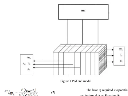
2.1.3 Heat and mass balance for the pad-end model
Figure 1 depicts the pad-end model for which the
heat and mass balance are derived. The change in the
sensible heat q is equal to the change in the enthalpy hc of
the air after passing through the pad. The Equation 7 is
given by:
(7)
The rate of evaporation MT could be expressed as
Equation 8:
MT= hDρaVa(Hp-Ho)PpPA/Va
= (hDρaVaMw)/(RoTabs) x (Pvs-Pva) PpPAPT/Va (8)
The heat Q required evaporating the water from the
pad in time dt is as Equation 9:
Q = MThfg = hfghDMwρaVa/(RoTabs) x (Pvs-Pva) PpPAPT/Va
(9)
where hfg = 2.503 x 10 6
– 2.38 x 10³ (Tabs-273.16)
273.16≤T(K)≤338.723 (Dzivama 2000).
At equilibrium, equating Equation 8 and Equation 9
give Equation 10:
Tp = Todb – (hfgMw(Pvs-Pva)) x Va 2ρa2
(Ca+WoCv) x (PpPAPT)
RoTabsρaCa(sc/pr)⅔Va
(10)
where ρaCa(sc/pr)⅔ = hꞌ/hD = the ratio of the
convective heat transfer to that of the mass transfer
coefficient. See Equation 11 and Equation 12.
(11)
Now
(12)
Kachhwah and Suhas (2010), presented a set of
equations (from Equation 13 to Equation 22) for the inlet
and outlet water temperatures associated with the
evaporative cooling process. These temperatures are
based on an elevated inlet water temperature entering the
absorbent materials above that of the ambient wet bulb
temperature. The correlation presented for heat transfer is
given as:
Nu = y x (Re0.8) x (Pr0.33) (13)
where y = 0.1 x (De 0.12
)
Reynold number, Re = ρa x μ x De (14)
μa
Prandtl number, Pr = cpa x μa (15)
Ka
(16)
De = (17)
α = (18)
NTU = hc x As (19)
ma x cpa
ϕ = 1 – exp (-1.07(NTU) 0.295) x α-0.556
x Mr -0.051
(20)
The exit Tdb is calculated as
η = ϕη1 (21)
where η1 = 1 – exp (-1.037NTU) (22)
The humidity ratio is calculated as Equation 23:
w2 = 0.62198Pwv2 (23)
Patm – Pwv2
The equations below (from Equation 24 to Equation
26) describe the effects of the independent variables ﴾pad
thickness, air velocity and water flow rate) on the storage
chamber temperature.
Tc = 3160.7PT 2
– 399.79PT + 31.54 (24)
Tc =3.0504+ 56.643 Va– 62.2 Va 2
+ 26.933 Va 3
-4 Va 4
(25)
Tc = 0.2542WR 4
– 2.8167 WR 3
+ 11.14 WR 2
– 17.796
WR + 28.449 (26)
where Ma is the mass of air, ρa is the density of air,
To is the inlet air temperature, To (wb) is the wet-bulb
temperature of the region, Wo is the humidity ratio of the
air, Mr is the water to air mass flow rate ratio,Tw1 is the
inlet water temperature, Tw2 is the outlet water
temperature, Tdb1 is the inlet air dry bulb temperature, Pva
is the partial vapour pressure of air, Pvs is the vapour
pressure of saturated air at the wet-bulb at the
temperature of the region, Patm is the atmospheric
pressure, Cv is the specific heat capacity of water vapour,
Ca is the specific heat capacity of air, Ro is the universal
gas constant, hfg is the latent heat of vaporization, Pa is
the density of air, the molecular weight of water ratio of
the convective heat and mass transfer is given by (h1/hD)=
(sr/pr)2/3, PT" is the pad thickness, Pp is the pad porosity,
PA is the pad surface area, Va is the air velocity and WR is
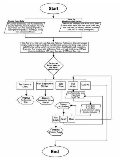
the water flow rate. A detailed algorithm to solve the
2.1.4 Description of the computer programme
The system is divided into three (3) sub systems
with three different user interfaces. Three popup windows will appear after the user enters ‘cool’ in the command
window of the program. Figure 3 to Figure 5 show the
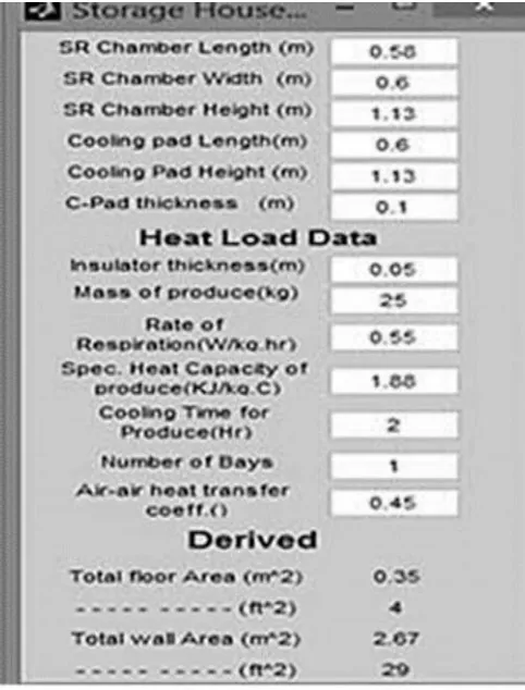
content of these three windows. The first window as
shown in Figure 3, is used to input and calculate the
dimensions of the storage chamber and the cooling pad.
Lines below the ‘Derived’ section as shown in Figure 3,
are the calculated results of the total floor area and the
Figure 3 The First window for the storage chamber and
heat load data
Figure 4 The Second window algorithm for dimension
psychrometric entrance air data and pad data
Figure 5 The Third window shows summary of
characteristics of the humidified air in the storage
chamber
Figure 4 shows the second window for the input of
data of the psychrometric properties of air and water
passing through the pad. Based on the input data, the
program will calculate the related values of the storage
chamber temperature, storage chamber humidity ratio and
outlet water temperature.
Figure 5 shows a result window with adiabatic
cooling values, a simulation of the internal air conditions
in the storage chamber, and the evaporative cooling
system performance efficiency. The first button calls up a
digital psychrometric chart to check the outdoor wet bulb
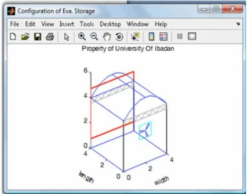
and dry bulb temperature with respect to the inlet air humidity ratio, as shown in Figure 6. The ‘close’ button closes the figure created by the ‘Draw Evaporative Storage’ option as shown in Figure 7. If the figure is not
closed, then the program automatically saves all the
current values as defaults for next ‘run’. The ‘Draw Evaporative Storage’ option makes use of some
parameters listed in Figure 5 to draw the storage chamber
layout. The ‘Data Table’ buttons enable the user to
Figure 6 The Fourth window shows digital psychrometric
chart
Figure 7 Evaporative cooling system storage layout
2.2 Experimental setup
For verification of the above mentioned model, the
solar power evaporative system as reported by Olosunde
et al. (2016) was used. The evaporative cooler consisted
of a pad end, a suction fan, a storage cabin, a water pump,
an overhead tank, a collection tank and pipes. The pad
was installed on one side of the cabin, and the suction fan
installed on the other side, opposite to the pad end. An
overhead tank was installed on the top of the cooler, from
which water dripped onto the pad through a lateral pipe
laid on top of the pad. There was a collection tank at the
bottom of the cooler to collect excess water from the pad.
The pump re-circulated the excess water back to the
overhead tank. The framework was of five different
thicknesses of 20, 40, 60 80 and 100 mm of size 600 x
1130 mm, corresponding to one side of the storage cabin.
See Figure 8.
Figure 8 Solar powered evaporative cooling storage
system
2.3 Analysis
A two-sample t-test using pooled variance was
performed to test if the hypothesis that the resulting
means of the modelled data and of the experimental data
were equal.
3 Results and discussion
3.1 Effect of the thickness of the pad on saturation
efficiency
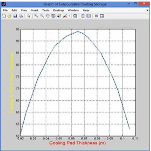
The effect of pad thickness on the storage chamber
temperature is shown in Figure 9. A cooling pad
thickness of 0.01 - 0.110 m was used to run the software.
The saturation efficiency increased as the thickness of the
decrease as the cooling pad thickness increased further
from 0.066 – 0.11 m. This change occurred because an
increase in the thickness of the pad tended to increase the
residence time of the air within the pad, thus creating a
longer period for the air-water contact. This phenomenon
meant that the air could possibly evaporate more water
due to the longer distance travelled and the residence time.
However, with a further increase in the pad thickness, the
air would become closer to being saturated as it travelled
through the pad, which would reduce the capacity of the
air to evaporate and absorb a greater amount of water
from the pad. Therefore, the efficiency decreased with a
greater pad thickness.
Figure 9 Effect of pad thickness on the saturation
efficiency
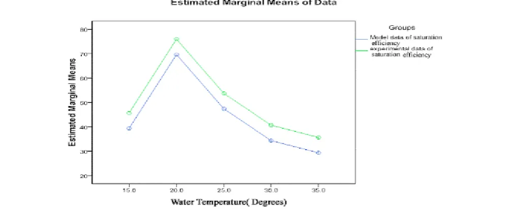
3.2 Effect of inlet water temperature on the saturation
efficiency
The effect of water temperature on the saturation
efficiency is presented in Figure 10. At inlet, water
temperature was between 17°C and 18°C and there was a
sudden increase in the saturation efficiency, while a
further increase in inlet water temperature beyond 18°C
resulted in a sudden drop in the efficiency. The sudden
increase occurred because the inlet water temperature was
lower than the wet bulb temperature. This result clearly
indicated that the performance of the evaporative cooling
was higher when the inlet water temperature was close to
the wet bulb temperature.
Figure 10 Effect of inlet water temperature on the
saturation efficiency
3.3 Effect of air velocity on the saturation efficiency
As the air velocity increased from 0.5 to 1.7 m/s, the
saturation efficiency increased. Between an air velocity of
1.7 to 1.85 m/s, the efficiency remained constant. A
further increase in the air velocity reduced the efficiency
as shown in Figure 11. The initial high rate of increase in
the saturation efficiency with increasing air velocity due
to the turbulent nature of the airflow at a high velocity
within the pad, i.e., the air could evaporate more water
and thus increase the efficiency. Air moving at a low
velocity would not be turbulent and only evaporate the
water in its path, which reduced the amount of water that
could be evaporated and hence reduced the efficiency of
the cooling system. However, a high velocity may reduce
the residence time of the air within the pad, which
resulted in a slight decline in the efficiency as the air
velocity increased further. A higher velocity tended to
pull water droplets out of the pad instead of evaporating
them, and this effect reduced the efficiency of the system.
These results are in agreement with the software
Figure 11 Effect of air velocity on the saturation
efficiency
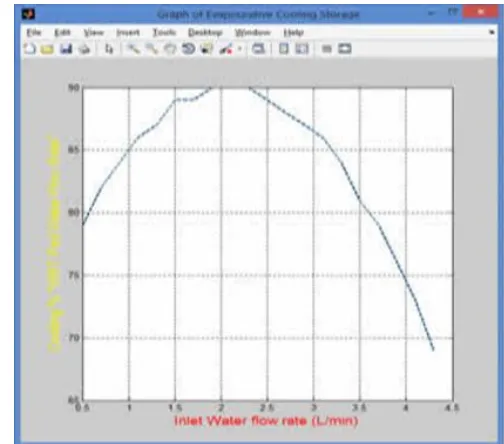
3.4 Effect of water flow rate on the saturation
efficiency
Figure 12 shows the effect of the water flow rate on
the saturation efficiency. The saturation efficiency
increased with an increase in the water flow rate, which
was obvious because a low water flow rate would leave a
dry spot where unsaturated air could pass directly through
the pad without evaporating water, thus increasing the
storage chamber temperature and reducing the efficiency.
The water may be inadequate to wet and saturate the pad.
As the water flow rate increases, the pad becomes wet
and closer to being saturated, i.e., the air evaporated more
water from the pad and, therefore, more cooling occurred.
The value of the saturation efficiency was observed to
decline slightly after a water flow rate of 2 L/min,
because at this flow rate the pad was excessively wet with
water. The excess water may block the pore spaces within
the pad fibres, thereby impeding the free flow of air
through the pad which reduced good evaporation.
Figure12 Effect of water flow rate on the saturation
efficiency
3.5 Comparison between the modelled data and the
experimental data of the four parameters of the
saturation efficiency
The hypotheses for this test are H0: μ1 = μ2 versus
Ha: μ1 ≠ μ2 or, in words, the following:
Null hypothesis (H0): There is no significant
difference between the experimental data and the
simulated data of the effects of Pad thickness, air velocity,
water flow rate and water temperature on the saturation
efficiency.
Alternative hypothesis (Ha): There is a significant
difference between the experimental data and the
simulated data of the effects of Pad thickness, air velocity,
water flow rate and water temperature on the saturation
efficiency.
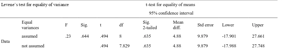
Figure 13 shows a comparison between the modelled
data and the experimental data of the saturation efficiency
as a function of the pad thickness. From the graph no
significant difference is observed between the respective
mean values of the modelled and experimental data of the
mean effect of the Pad thickness on the saturation
efficiency, t (5) = 0.494, p = 0.635. (p > 0.05),- as
The relationship between the modelled data and the
experimental data of the saturation efficiency versus the
air velocity is described in Figure 14. From the graph, no
significant difference was observed for the mean effect of
air velocity on the saturation efficiency for the
experimental data and the simulation data, t (5) = 1.639, p
= 0.140. (p > 0.05), as presented in Table 2
Figure 13 Comparison between modelled data and experimental data of saturation efficiency against pad thickness
Table 1 Independent samples test of the pad thickness against the modelled and experimental data of the
saturation efficiency
Levene’s test for equality of variance t-test for equality of means 95% confidence interval Equal
variances F Sig. t df
Sig. 2-tailed
Mean
diff. Std error Lower Upper Data
assumed .23 .644 .494 8 .635 4.88 9.879 -17.901 27.661 not assumed .494 7.829 .635 4.88 9.879 -17.988 27.748
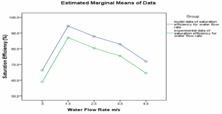
Additionally, the relationship between the modelled
data and the experimental data of the saturation efficiency
versus the water flow rate is described in Figure 15. From
the graph, no significant difference was found between
the modelled and experimental mean values. Thus, the
mean effect of the water flow rate on the saturation
efficiency for both the experimental data and the
simulation data were not significantly different, t (5) =
1.013, p = 0.341. (p > 0.05),- see Table 3 for the details.
Figure 16 shows the relationship between the
modelled data and the experimental data of the saturation
efficiency versus water temperature. From the graph, no
significant difference was observed between their
respective mean values. Thus, the mean effect of water
temperature on the saturation efficiency for both the
experimental results and the simulation result were not
significantly different, t (5) = -0.597, p = 0.567. (p >
0.05),- see Table 4 for the details.
Table 2 Independent samples test of the air velocity against the modelled and the experimental data of the
saturation efficiency
Levene’s test for equality of variance t-test for equality of means
95% confidence interval
Equal
variances F Sig. t df
Sig. 2-tailed
Mean
diff. Std error Lower Upper Data
assumed .261 .624 1.64 8 .140 5.64 3.442 -2.297 13.577 not
assumed .494 7.41 .143 5.64 3.442 -2.407 13.687
Figure 15 Comparison between modelled data and experimental data of saturation efficiency against water flow rate
Table 3 Independent samples test of the water flow rate against the modelled and the experimental data of
the saturation efficiency
Levene’s test for equality of variance t-test for equality of means
95% confidence interval
Equal
variances F Sig. t df
Sig. 2-tailed
Mean
diff. Std error Lower Upper Data
4 Conclusions
The developed program is simple and efficient, with
a suitable interface for the input of the necessary data,
and the program provides sufficient information to
optimize the design of an evaporative cooling system for
the storage of fruits and vegetables. The results of the
comparison between the modelled data and the
experimental data indicated that there was no significant
difference between the software generated data and the
experimental data of the saturation efficiency versus Pad
thickness – mm (p = 0.635), Air Velocity - m/s (p =
0.140), Water Flow Rate - L/min (p = 0.341) and Water
Temperature 0C (p = 0.567) at α = 0.05 significant level
and 95 % confidence interval.
Hence, the program provides the capability to
identify the working conditions based on the appropriate
figures, thus demonstrating the effect of the cooling pad
thickness, water flow rate, inlet water temperature, air
velocity, number of cooling segments and water to air
flow rate on the storage chamber temperature, the storage
chamber humidity ratio and the saturation efficiency.
References
Boyette, M. D., L. G. Wilson, and E. A. Estes. 2010. Postharvest handling and cooling of fresh fruits, vegetables and flowers for small farms. Leaflets 800-804. North Carolina Cooperative Extension.
Camargo, J. R., C. D. Ebinuma, and S. Cardoso. 2003. A mathematical model for direct evaporative cooling air conditioning systems. Engenharia Termica, Curitiba,
4(1):30-34.
Figure 16 Comparison between modelled data and experimental data of saturation efficiency against water
temperature
Table 4 Independent samples test of the water temperature against the modelled and the experimental data of
the saturation efficiency
Levene’s test for equality of variance t-test for equality of means
95% confidence interval
Equal
variances F Sig. t df
Sig. 2-tailed
Mean
diff. Std error Lower Upper
Data
assumed .357 .567 -.597 8 .567 -6.30 10.55 -30.63 18.027 not
Cui, X., K. J. Chua, and W. M. Yang. 2014. Use of direct evaporative cooling as pre-cooling unit in humid tropical climate: an energy saving technique. The 6th International Conference on Applied Energy – ICAE 2014. Energy Procedia, 61(2014):176-179.
doi:10.1016/j.egypro.2014.11.933.
Dzivama, A.U. 2000. Performance evaluation of an active cooling system for the storage of fruits and vegetables. Ph.D. Thesis, Department of Agricultural Engineering, University of Ibadan, Ibadan.
Fang, W., D. S. Fon, Z. H. Jian, and D. C. Wang. 2001. Re-development of Psychrometric software using Visual C++ and MATLAB. Proceedings of the International Forum for Vegetable Production. Amen, China.
Kachhwah, S. S., and P. Suhas. 2010. Heat and mass transfer study in a direct evaporative cooler. Journal of Scientific and Industrial Research, 69(9):705-710.
Kulkarni, R. K., and S. P. S. Rajput. 2011. Comparative performance of evaporative cooling pads of alternative materials. International Journal of Advanced Engineering Sciences and Technologies, 10(2):239-249.
Ndukwu, M. C., and S. I. Manuwa. 2014. Review of research and application of evaporative cooling in preservation of fresh agricultural produce. International Journal of Agricultural and Biological Engineering, 7(5):85-102.
Ndukwu, M. C., S. I. Manuwa, O. J. Olukunle, and I. B. Oluwalana. 2013. Development of an active evaporative cooling system for short-term storage of fruits and vegetables in a tropical climate. Agricultural Engineering International: CIGR Journal, 15(4):307-313.
Ndukwu, M. C. 2011. Development of a clay evaporative cooler for fresh fruits and vegetables preservation. Agricultural Engineering International: CIGR Journal, 13(1):1-8.
Olosunde, W. A., A. K. Aremu, and D. I. Onwude. 2016.
Development of a solar powered evaporative cooling storage system for tropical fruits and vegetables. Journal of Food Processing and Preservation, 40(2):279-290
Olosunde, W. A. 2015. Performance of a forced convection evaporative cooling storage system for selected tropical perishable crops. Ph.D. Thesis, Department of Agricultural Engineering, University of Ibadan, Ibadan.
Olosunde, W. A., J. C. Igbeka, and T. O. Olurin. 2009. Performance evaluation of absorbent materials in evaporative cooling system for the storage of fruits and vegetables.
International Journal of Food Engineering, 5(3):1-15. Sirelkhatim, A. K. and A. A. Emad. 2012. Improvement of
evaporative cooling system efficiency in greenhouses.
International Journal of Latest Trends in Agriculture and Food Sciences, 2(2):83-89.
Taye, S. M. and P. F. Olorunisola. 2011. Development of an evaporative cooling system for the preservation of fresh vegetables. African Journal of Food Science, 5(4):255-266. Van der Walt, N. T., and R. Hemp. 1989. Thermometry and
temperature measurements in environmental engineering in South African Mines. Chp 17. The Mine Ventilation Society of South Africa.
Wang, D. C., W. Fang, and D. S. Fon. 2002. Development of a digital psychrometric calculator using MATLAB. Acta Horticulturae, 578:339-344.
DOI: 10.17660/ActaHortic.2002.578.42
Wei, Z., and S. Geng. 2009. Experimental research on direct evaporative cooling of organic padding contamination.
Contamination Control & Air-Conditioning Technology,
22-26.