Improvement of DV-Hop Algorithm Based on
RSSI Ratio Correction
https://doi.org/10.3991/ijoe.v14i05.8647
Xiaoying Yang!!", Wanli Zhang, Qixiang Song
Suzhou University, Suzhou, China
Abstract—This paper aims to improve the positioning accuracy of the tradi-tional DV-hop algorithm in networks of uneven node distribution. For this pur-pose, an improved algorithm was proposed that reduces the errors in terms of the hop count, the mean single-hop distance of anchor nodes and the mean sin-gle-hop distance of unknown nodes. Specifically, the hop count was modified based on the RSSI value of the node and the critical RSSI ratio; the mean sin-gle-hop distance of anchor nodes was corrected based on the ratio of the single-hop RSSI path length between two nodes to the mean single-single-hop RSSI path length (i.e. the correction factor); the mean single-hop distance of unknown nodes was divided into two sections to achieve better estimation of the distance between anchor nodes and unknown nodes. The simulation results indicate that the improved algorithm boasts better positioning accuracy and stability than the contrastive algorithms, with the addition of a few computing and communica-tion overhead. The research findings shed new light on the accurate posicommunica-tioning of nodes in wireless sensor networks (WSNs).
Keywords—DV-hop algorithm, received signal intensity indication (RSSI), hop count, mean single-hop distance
1
Introduction
Node location information is essential to various applications of wireless sensor network (WSN), including but not limited to target, detection, target tracking, and automatic configuration of network topology [1]. In light of the ranging requirement, the existing positioning algorithms are either ranging-based or ranging-free [2]. The ranging-based algorithms demand strong hardware capacity and have high positioning accuracy. The typical examples are received signal intensity indication (RSSI), angle of arrival (AOA), time of arrival (TOA), and time difference on arrival (TDOA). In contrast, the ranging-free algorithms, featured by low hardware requirements, and positioning accuracy, mainly include DV-hop algorithm, centroid algorithm and ap-proximate point in triangle (APIT) algorithm. With low cost and no additional hard-ware, the ranging-free algorithms are more suitable for largescale WSNs [3].
dis-tance between the nodes, and the path is not necessarily linear. Errors may occur in the distance estimation between anchor nodes and unknown nodes, owing to the fol-lowing factors. (1) The hop count error: the hop count is considered as 1 as long as the internodal distance falls in the communication radius; (2) The slight error in the mean single-hop distance of anchor nodes: the mean distance equals the mean esti-mated distance of all transmission paths between anchor nodes and unknown nodes; (3) The huge error in the mean single-hop distance of unknown nodes: the mean dis-tance is related to the degree of curvature of the shortest transmission path, which is uncertain if that path covers a long distance. It is the distance estimation error that drags down the positioning accuracy.
Over the years, the distance estimation error has been treated from three aspects. For instance, Reference [4] introduces the deviation factor to correct the hop count error. Reference [5] modifies the mean single-hop distance of anchor nodes and un-known nodes to improve positioning accuracy. Reference [6] rectifies the internodal hop against the RSSI value received by the neighboring nodes of anchor nodes, and optimizes the mean single-hop distance of anchor nodes. Following the method of least squares, Reference [7] derives the total error in the mean single-hop distance of anchor nodes, sets the mean offset of the mean single-hop distance to zero, and ob-tains the mean single-hop distance that minimizes the total error. Reference [8] relies on the error in mean single-hop distance to correct the mean single-hop distance be-tween anchor nodes and unknown nodes. Reference [9] adjusts the hop count using the RSSI method, and identifies the mean single-hop distance of unknown nodes by weighting the mean single-hop distance of each anchor node. Taking the RSSI value received by anchor nodes at each hop as the reference value, Reference [10] revises the hops from anchor nodes to unknown nodes by the RSSI ratio. By the above meth-ods, the positioning accuracy can be improved by a certain degree, but the results are still undesirable.
To further enhance the positioning accuracy, this paper proposes an algorithm that reduces the errors in such three aspects as the hop count, the single-hop distance of anchor nodes and the mean single-hop distance of unknown nodes.
2
DV-hop algorithm
2.1 Positioning process
Proposed by Niculescu et al. [11, 12], the DV-hop algorithm estimates the distance between anchor nodes and unknown nodes by multiplying hop count with the mean single-hop distance, and then calculates the coordinates of unknown nodes with three-sided measurement. The positioning process is explained below.
Each anchor node broadcasts packets {idi, xi, yi, hop} containing its ID,
The mean single-hop distance of each anchor node is calculated by:
!
!
" "
# + # =
i
j j
i
j i j i j
i x x y y hops
hopsize ( )2 ( )2 /
(1) where (xi, yi), (xj, yj) and hopsj are the coordinates of anchor node i, the coordinates
of anchor node j, and the minimum hop count between the two nodes, respectively. Each unknown node can estimate its distance from the anchor nodes by multiplying the mean single-hop distance of the nearest anchor node with the minimum hop count. The coordinates of each unknown node can be estimated with its distances to 3 or more anchor nodes.
2.2 Error analysis
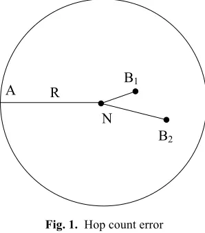
From the positioning process of the traditional DV-hop, it can be seen that the hop count is considered as 1 as long as the internodal distance falls in the communication radius. As shown in Fig. 1, N is an unknown node, B1 and B2 are anchor nodes, and R is the communication radius. Both the hop count between N and B1 and that be-tween N and B2 are 1. The hop count does not reflect the actual distance. In this case, the mean single-hop distance is reasonable only if the nodes are evenly distributed. Errors are inevitable if the network has an irregular topology.
R B1
N
B2 A
Fig. 1. Hop count error
3
Improved DV-hop Algorithm
3.1 RSSI ranging model
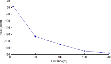
The RSSI distance masked dissipation model was adopted to correct the hop count and the mean single-hop distance between nodes. The path loss sub-model takes a near distance d0 as the reference to predict the mean signal intensity at distance d. The
proportional relationship between the two distances can be expressed as:
n d d d PL
d
PL ( )
) (
)
( 0
0 =
(2) Find the logarithm on the left and right:
0
0) 10 lg
( ) (
d d n d PL d
PL = !
(3) where PL(d) is the RSSI value at distance d (dBm); n is the path loss coefficient (2~4); PL(d0) is the RSSI value at the reference distance d0. As shown in Fig. 2, the
RSSI value varies with distances.
Fig. 2. Relationship between RSSI value and distance
3.2 Correction of hop count
By the traditional DV-hop algorithm, the hop count is considered as 1 as long as the internodal distance falls in the communication radius, sowing the seed of huge errors (Fig. 1). To prevent the errors, the RSSI technique was introduced to correct the hop count.
It can be seen from Fig. 2 that the internodal distance is negatively correlated with the RSSI value. Since the signal intensity at a node is usually negative, the RSSI ratio was employed to approximate the distance ratio. Suppose two nodes receive the in-formation broadcasted from the same anchor node. Let RSSI1 and RSSI2 be the signal
intensities at each of the two nodes, and d1 and d2 be the distance between the anchor
2 1 2 1 d d RSSI RSSI ! (4) Let us denote the hop count of the node on the communication radius as 1, and the ideal distance as R. Taking the RSSI value at R is as the critical value RSSIth, the
cit-ical value can be expressed as:
0
0) 10 lg
( d R n d PL RSSIth = !
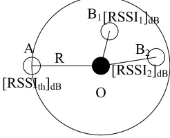
(5) The principle of the critical RSSI ratio is illustrated in Fig.3.
O A
B1
R [RSSIth]dB
B2
[RSSI1]dB
[RSSI2]dB
Fig. 3. Principle of critical RSSI ratio
The critical RSSI ratio can be calculated by:
! " ! # $ = % = ) ( 1 d PL RSSI RSSI RSSI hop i th i i (6) If hopi=1, the node falls on the communication radius and has a hop count of 1.
The node A in Fig. 3 is such an example. If hopi <1, the node falls within the
com-munication radius and has a hop count less than 1. The nodes B1 and B2 in Fig. 3 are such examples.
In this way, the hop count of the nodes within the communication radius can be expressed as decimals. The new expression is closer to reality, reduces the hop count error, and thus enhances the accuracy of the mean-single hop distance.
3.3 Correction of mean single-hop distance of anchor nodes
To eliminate the influence, the mean single-hop distance was corrected based on the ratio of the hop RSSI path length between two nodes to the mean single-hop RSSI path length (i.e. the correction factor).
Considering the RSSI value of each hop recorded by each node and the cumulative RSSI value up to the current hop, the correction factor can be established by the for-mula below:
avg i
i
=
RSSI
/
RSSI
!
(7)where RSSIi is the signal intensity at node i; RSSIavg is the mean signal intensity at
node i in the case of mean single-hop distance broadcasting from the anchor node. The RSSIavg can be obtained as follows:
n
n
RSSI
RSSI
RSSI
RSSI
avg=
(
1
)
+
(
2
)
+
!
+
(
)
(8) Then, the correction factor of the mean single-hop distance is multiplied by the mean single-hop distance to yield the corrected mean single-hop distance. If the hop count between unknown nodes and anchor nodes is denoted as n, then the corrected mean single-hop distance is:
Hopsize
Hopsize
Hopsize
e
Hopsiz
"
=
#
1!
+
#
2!
+
!
+
#
n!
RSSI Hopsize RSSI RSSI RSSI RSSI RSSI avg n avg avg ! + + +
=( 1 2 ! )
Hopsize RSSI RSSI n k avg k ! =
"
= ) ( 1Hopsize
RSSI
n
RSSI
avg!
=
(
)
(9) The above steps make it possible to correct the mean single-hop distance of anchor nodes according to the cumulative signal intensity (RSSI(n)), mean signal intensity (RSSIavg) and mean single-hop distance (Hopsize). The values of these parameters aresaved in the information table.
3.4 Correction of mean single-hop distance of unknown nodes
In the traditional DV-hop algorithm, the mean single-hop distance of the nearest anchor node is regarded as the mean single-hop distance of unknown nodes. This expedient measure cannot reflect the overall situation of the network.
In the near range of unkown nodes, the mean single-hop distance is weighted by the mean single-hop distance of anchor nodes around such nodes. Within the range of the unknown nodes, the mean single-hop distance is adjusted to be the weighted sum of the anchor nodes and the mean single-hop distance of the distant anchor nodes.
The estimated distance is corrected as follows. When anchor nodes broadcast over the mean single-hop distance, each unknown node receives the mean single-hop dis-tance of all anchor nodes. The hop count between anchor nodes to the unknown node is ranked in ascending order, and the m smallest hop counts are selected. The corre-sponding mean single-hop distance are denoted as Hopsize1, Hopsize2, …, Hopsizem.
Then, the weight of mean single-hop distance can be calculated by:
!
= + " = m i i i i hop hop Max W 1 1 (10) where hopi is the hop count between an unknown node and anchor node i; Max isthe maximum hop count.
In this way, each node is assigned a weight negatively correlated with the distance. The anchor node closer to the unknown node has a greater effect on the calculation of the mean single-hop distance. Thus, the anchor nodes are grouped rationally based on their contributions to the calculation. The mean single-hop distance of unknown nodes was also divided into two parts.
If the unknown node is within the range.
If the distance to anchor nodes is within m hops, then the mean single-hop distance of the unknown node can be calculated by:
i m
i i
p
W
Hopsize
Hopsize
!
=
=
1 (11)
The distance from the unknown node to M anchor nodes can be obtained by:
i p pi
Hopsize
hop
D
=
!
(12)If the distance to anchor nodes is greater than m hops, then the mean single-hop distance of the unknown node can be calculated by:
q Hopsize Hopsize Hopsize Hopsize q q ! + +
= 1 2
(13) where q is the number of anchor nodes with a distance greater than m hops. The distance from the unknown node to these nodes can be obtained by:
)
(
j m qm p
qj
Hopsize
hop
Hopsize
hop
hop
4
Workflow of the Improved DV-hop Algorithm
The workflow of the improved DV-hop algorithm is detailed below.
(1) Each anchor node sends packets {ID, (x, y), hop, RSSIi, RSSI(sum)} to the
net-work, where ID is the node number, (x, y) are the coordinates, hop is the corrected hop count (initial value=0), RSSIi is the signal intensity at each neighboring node
(initial value=0), and RSSI(sum) is the cumulative signal intensity of all nodes up to the current hop (initial value=0).
(2) When the direct neighboring node receives a packet, it reads the signal intensity () from the register of the wireless node chip. The RSSI is set as the signal in-tensity when the node receives the packet, =. Then, the hop count is updated in the packet as hop=hop+RSSI1/RSSIR. Among all the packets of the same ID, the node only saves the one with the smallest hop count, and forwards the rest of the packets.
(3) The direct neighboring node continues to send packets to its neighboring nodes. Upon receiving a packet, the node changes the packet information to {ID, (x, y), hop, RSSI2, RSSI1+RSSI2}, and updates the hop count hop=hop+RSSI2/RSSIR. Again,
among all the packets of the same ID, the node only saves the one with the smallest hop count, and forwards the rest of the packets.
(4) Repeat Step (3) until the hop count no longer changes. The final information in each packet is {ID, (x, y), hop, RSSIn, RSSI1+RSSI2+……+ RSSIn}. The mean
single-hop distance, calculated by formula (1), and the mean signal intensity, calculated by formula (8) will be broadcasted in flooding mode.
(5) The correction factor of each hop is computed by formula (7), and the mean single-hop distance is corrected by formula (9) according to the correction factor. Then, the corrected mean single-hop distance will be broadcasted to the network.
(6) The unknown nodes receive the mean single-hop distance of all the anchor nodes. Then, the hop counts between the anchor nodes and the unknown nodes are ranked in ascending order, and the m smallest hop counts are selected. The weight of each node is calculated by formula (10). Formulas (12) and (14) are used to calculate the distance between the nearer and farther nodes.
(7) The coordinates of unknown nodes are obtained by maximum likelihood esti-mation.
5
Algorithm Simulation and Result Analysis
5.1 Simulation environment and parameter setting
The anchor nodes and unknown nodes are randomly distributed in a network with an area of [0100] * [0100]. The anchor nodes were randomly selected, and assigned with the same communication radius R. To eliminate the errors resulted from random node distribution, 100 simulation experiments were performed in the same network environment to obtain the mean values.
Normalized positioning error is an indicator of the positioning accuracy of the al-gorithm [13]. Let (xt, yt) and (xe, ye) respectively be the actual location and estimated
location of a node. Then, the mean positioning error of all unknown nodes is:
KN
y y x x error
K
j N
i t e t e
!!
= =
"
+
"
= 1 1
2
2 ( )
) (
(15) The normalized positioning error is defined as:
R
error
r
erro
!
=
/
(16)Hence, the positioning accuracy is (1-error’)*100%.
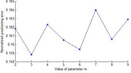
During the simulation experiments, the number of network nodes was set to 100, the proportion of anchor nodes to 30%, and the communication radius to 30m. Fig. 4 shows the variation in the positioning accuracy with the value of M.
Fig. 4. Relationship between positioning accuracy of M value
It is clear that the normalized positioning error varies slightly around 16% with the alteration of M value, and does not increase with M value. For better positioning accu-racy, the computing load should be minimized. Hence, the value of M was set to 3 in the simulation experiments.
5.2 Effect of the proportion of anchor nodes on positioning accuracy
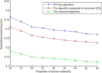
increased gradually from 10% to 50% by a step of 10%. The communication radius R was set to 30m. Fig. 5 presents the normalized location errors of the three algorithms.
According to Fig. 5, the positioning errors of the three algorithms all gradually de-clined with the increase in the proportion of anchor nodes. When the proportion of anchor nodes fell between 10% and 20%, the positioning errors plunged rapidly. In this case, the positioning accuracy hinges on the anchor node density or network con-nectivity. After the proportion of anchor nodes surpassed 20%, the positioning errors were gradually stabilized. Overall, the improved DV-hop algorithm had a 17.56% higher positioning accuracy than the traditional DV-hop algorithm and a 12.87% higher positioning accuracy than the algorithm in Reference [10]. The performance edge is attributable to the modification of the minimum internodal hop count and the correction of the mean single-hop distances of anchor nodes and unknown nodes in the improved algorithm. In this way, fewer errors are caused by the minimum hop count and mean single-hop distances. Thus, the distance between unknown nodes and anchor nodes are closer to the actual distance. As shown in Fig. 5, the curve of the improved algorithm is smoother and more stable than the curves of the contrastive algorithms.
Fig. 5. Relationship between the proportion of anchor nodes and positioning error
5.3 The effect of the number of nodes on positioning accuracy
Fig. 6. Relationship between the number of nodes and positioning error
It is observed that the positioning errors of the three algorithms decreased with the increase in the number of nodes. The curves of these algorithms were relatively smooth. This means the number of nodes has little to do with the positioning accuracy when the proportion of anchor nodes remains constant. However, the improved algo-rithm obviously outperformed the other two algoalgo-rithms in positioning accuracy. The lead was 15.5% over the traditional DV-hop algorithm and 8.3% over the algorithm in Reference [10].
5.4 The effect of communication radius on positioning accuracy
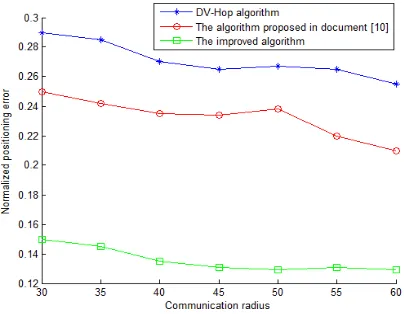
The number of network nodes was fixed at 100, and the proportion of anchor nodes was kept at 30%. Then, the communication radius was adjusted to compare the posi-tioning accuracy of the improved algorithm, the traditional DV-hop algorithm and the algorithm in Reference [10]. Fig. 7 illustrates the results of the simulation experi-ments.
It can be seen from Fig. 7 that the positioning error of the improved algorithm was much lower than that of the traditional algorithm and the algorithm in Reference [10]. Since all nodes in the network were randomly distributed, the positioning errors decreased as the communication radius widened. Compared to the other two algo-rithms, the improved algorithm had limited vibration such that the positioning error decreased steadily despite the changes in communication radius. The positioning accuracy of the improved algorithm was 14.4% higher than that of the traditional algorithm and 8.6% higher than that of the algorithm in Reference [10]. The results demonstrate that our algorithm boasts better stability and performance, and is more adaptive to the environment.
6
Conclusion
To overcome its huge positioning error in networks of random node distribution, the traditional DV-hop algorithm was improved in three phases. Specifically, the hop count was adjusted by the RSSI value, the mean single-hop distance of anchor nodes was modified by the correction factor, and the mean single-hop distance of unknown nodes was calculated in two parts. The simulation results show that, the improved algorithm boasts better positioning accuracy than the traditional algorithm and the algorithm in Reference [10], with the addition of a few computing and communica-tion overhead. The future research will attempt to reduce the computing load without sacrificing the positioning accuracy, so that the improved algorithm has a better appli-cation potential.
7
Acknowledgment
The study of our work is supported in part by Anhui University Provincial Natural Science Research Project (No. KJ2016A777), Anhui provincial outstanding young talent support program (No. gxyq2017093), outstanding academic and technical backbone of Suzhou University (No. 2016XJGG12).
8
References
[1] Shen J., Molisch A.F., Salmi J. (2012). Accurate Passive Location Estimation Using TOA Measurements. IEEE Transactions on Wireless Communications, 11(6), 2182-2192. https://doi.org/10.1109/TWC.2012.040412.110697
[2] Oguejiofor O.S., Aniedu A.N., Ejiofor H.C., Okolibe A.U. (2013). Tilateration Based Lo-calization Algorithm for Wireless Sensor Network. International Journal of Science and Modern Engineering, 1(10), 21-27.
[3] Tomic S., Mezei I. (2016). Improvements of DV-Hop localization algorithm for wireless sensor networks. Telecommunication Systems, 61(1), 93-106. https://doi.org/10.1007/s1 1235-015-0014-9
[5] Fang W.S., Lei G.X. (2015). A DV-HOP Algorithm Based on the Ratio between Node RSSI and the Critical RSSI Hop Correction and Hop Distance Revaluation. Chinese Jour-nal of Sensors and Actuators, 28(8), 1244-1248.
[6] Zhou X.B. (2011). Weighted DV-HOP positioning method based on RSSI in wireless sen-sor networks. computer engineering and applications, 47(14), 109-111.
[7] Lin J.Z., Chen X.B., Liu H.B. (2008). Iterative location algorithm for wireless sensor net-works based on the average hop distance correction. Journal of communications, 30(10), 107-112.
[8] Chen H. (2008). An improved DV-Hop localization algorithm with reduced node location error for WSNs. IEICE Transactions on Fundamentals of Electronics Communications and Computer Sciences, E91-A(8), 2232-2236. https://doi.org/10.1093/ietfec/e91-a.8.2232 [9] Wu N., Liu F.A., Wang S.X. (2015). Algorithm for Locating Nodes in WSN Based in
Modifying Hops and Hopping Distances. Microelectronics & Computer, 32(1), 91-95 https://doi.org/10.1016/j.mee.2015.02.039
[10] Yang X., Pan W. (2013). DV-Hop localization algorithm for wireless sensor networks based on RSSI ratio improving. Transducer and Microsystem Technologies, 32(7), 126-128, 135.
[11] Niculescu D., Nath B. (2003). DV based positioning in ad hoc networks. Kluwer Journal of Telecommunication Systems, 22(1-4), 267-280. https://doi.org/10.1023/A:10234 03323460
[12] Arivubrakan P.A., Dhulipala V.R.S. (2012). Energy consumption Heuristics in wireless sensor networks. Proceedings of the IEEE International Conference on Computing, Com-munication and Applications, 53(8), 1-3. https://doi.org/10.1109/ICCCA.2012.6179194 [13] Pan Z.J., Liu W.C., Luo Z., Yang H. (2016). Improvement of DV-Hop localization
algo-rithm for wireless sensor network. Computer Engineering and Design, 37(7), 1701-1704, 1740.
9
Authors
Xiaoying Yang is with the College of Information Engineering, Suzhou Universi-ty, Suzhou, China.Associate Professor, research field: target location in Wireless Sensor Networks.
Wanli Zhang is with College of Information Engineering, Suzhou University, Su-zhou, China.Associate Professor, research field: target tracking in Wireless Sensor Networks.
Qixiang Song is with the College of Information Engineering, Suzhou University, Suzhou, China.Associate Professor, research field: computer network.