Emergency Notification Using Combination Algorithm with Recognition ECG Signal

Emergency Notification Using Combination Algorithm

with Recognition ECG Signal

https://doi.org/10.3991/ijoe.v16i05.12707

Kittimasak Naijit

Chandrakasem Rajabhat University, Bangkok, Thailand [email protected]

Abstract—Intensive Care Unit (ICU) Rooms usually have several detectors attached to each patient providing intensive care, and several processors control and interpret. If the processor detects an abnormality, the medical professional office will be alerted. Nevertheless, many patients with heart disease are con-cerned with day-to-day behaviors such as hard work, battle, exercise, shock, fight, and war. Become due to clinical depression and erectile impotence this in-duces anxiety and fear. The boundaries of your heart muscle and coronary strength are unclear. They want a warning that is quick and accurate before they lose control. We develop signal recognition for an algorithm that is very fast and accurate. It helps alert patients to avoid the operation of risk. Nevertheless, it is able to transfer information from the heartbeat network to the doctor's guidance system. The research would analyze the 200 signals from multiple ECG signals. Integration Component Diagnosis (ICD) is capable of extraordinary reliability of identification than the 17.10-41.93 average percentage of the Automata Matching Process which takes less time than the other 29.37 average percentage process and can alert within 12 seconds. It cannot be identified in a pattern other than without the detection of an ECG signal. In the experimental, the signal is used to distinguish 20 ECG signal patterns.

Keywords—Emergency notification, combination algorithm, ECG signal

1

Introduction

compact data for efficient processing are standard for all ECG methods of study, re-gardless of the ECG diagnosis, stress testing, external surveillance, or intensive care surveillance. [7]Highly inadequate pumping capacity for blood flow controls is used to meet the requirements of the body, also known as congestive heart failure. The body, known as congestive heart insufficiency, is using extremely inadequate pumping ca-pacity for blood flow controls.

Fig. 1. Patients Risk for Heart Failure

In figure 1, heart failure may result in a number of symptoms including shortness of breath, swelling of the legs, and intolerance to exercise. Echocardiography and blood tests have been associated with the disease. This is a test performed in an office physi-cian where the body surface of the resting patient records 12 different potential differ-ences or ECGs. [15][23] Adding that we use another set of potential body surface as inputs to a three-dimensional vector model of cardiac excitation. The result is a sche-matic illustration of the excitement of the heart or a cardiogram of the wave. Neverthe-less, ECG leads are tracked or recorded for life-threatening variations in the rhythm of the heartbeat for long-term observation in the intensive care unit or on out patients. [4][10] ECG interpretation techniques have been developed initially and are now used in electronic machine computing. The ECG was sent to the device from remote hospital locations using a specially designed ECG acquisition cart that could be transported to the bedside of the patient. [9] As technologies progressed, microcomputers installed within the hospital assumed the role of the remote big computer. [23] The ECG acqui-sition cart continued to include an integrated microprocessor to enable the processing of the ECG. [21] When the ECG was a noise signal, the interpretation algorithm had an increased failure rate. Through running digital signal processing algorithms, the micro-processor improved the signal to noise ratio to eliminate background drift and attenuate liner interference. This research proposes: 1). A framework for data operation in rapid ECG analysis. 2). A classification algorithm using optimization analysis which is used for the extraction of features and for the recognition of the ECG signal.

2

Methodology

2.1 Signal combination algorithm

ECG wave pattern: We use classification methods for the pattern of identification in the ECG signal, which is quite similar to the process of machine recognition. [5] We use cross-correlation patterns to distinguish different signal patterns. The signals asso-ciated are the wave pattern forms of two signals that complement each other. The cor-relation coefficient is a function that specifies the degree of functionality between the two signal shapes of the ECG wave pattern recognition system used by Integration Component Diagnosis (ICD) for pattern recognition.

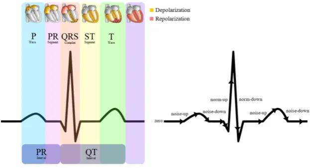
Automata template matching: We use a series of tokens that would represent a standard ECG. A set of tokens is an interface to the finite state automata. The series of tokens must be derived from the information of the ECG signal. This is achieved by generating a sequence of differences in the input information. The algorithm can now allocate a wave pattern token to each of the groups formed previously based on the values of the number and the sum of the differences in each group. We use ranges of QRS up-wards or down-wards, and then a norm-up or norm-down token is created for that class of differences. The QRS is the combination of three of a typical ECG's graph-ical deflections. [19] If the values of number and sum do not fall within this range, a noise-up or noise-down token will be created. The zero token is created if the sum for a group of differences is zero. The algorithm reduces the information of the ECG signal to a series of tokens that can be fed to finite state automata for QRS detection. [17] It's a moderate pattern of ECG detection. (Figure 2)

Fig. 2. Automata Template Matching

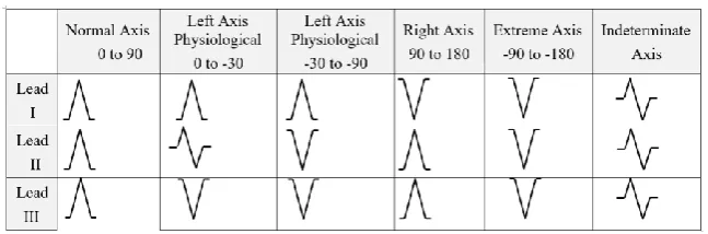
Table 1. QRS polarity in leads I, II, and III

2.2 Wave pattern of ECG signal recognition

The ECG is one of all medicine's most common, enduring, and important tests. It is easy to perform, non-invasive, yields tests quickly, and is useful to treat thousands of heart conditions. Lately, the ECG has become even more important because a specific ECG trend, called ST elevation, is a strong indication that there has been a severe heart attack, and more emphasis than ever is placed on handling heart attacks as soon as pos-sible. The ECG will not necessarily be part of a physical routine, but you will almost certainly get an ECG if you need medical attention because you have chest pain, sudden unexplained shortness of breath, or other symptoms that suggest a possible heart attack. (Table 2)

Table 2. Wave Pattern of ECG Signals

ECG Signal Wave Pattern ECG Signal Wave Pattern

Sinus Rhythm Wandering

Pacemaker

Sinus Bradycardia Paced Atrial

Sinus Tachycardia Accellerated

Idioventricular

Sinus Arrthythmia

Ventricular Fibrillation

Sinus Exit Block NSR with First _{Degree AV Block}

Sinus Arrest Second Degree AV

Block Type II

Premature Arial Second Degree AV

Block with 2:1

Supraventricular

Tachy-cardia Third Degree AV Block

Atrial Fibrillation Premature

Junctional Complex

Sinus Rhythm also as normal sinus rhythm (NSR) or regular sinus rhythm (RSR) is the most common adult rhythm with rates ranging from sixty to one hundred per minute. The QRS is most frequently narrow with upright P waves in Lead II. [20] It is a standard heart beat rhythm that compares each time in the first level warning.

Sinus Bradycardia can be well handled by healthy adults at speeds greater than 50 per minute.Due to an optimal volume of cardiac stroke that requires less HR to yield acceptable cardiac output, athletes may routinely be in Sinus bradycard. Sinus brady-cardia may also stem from vagal pressure or from Sick Sinus Syndrome. Wait for a short QRS in Lead II with upright P waves.

Sinus Tachycardia is most often the result of such as pain fever, increased sympa-thetic stimulation, hypovolemia, and increased oxygen demand. The most common symptom of Sinus Tachycardia is elevated sympathetic pressure such as high fever, increased demand for oxygen, and hypovolemia. It usually has a narrow QRS. Often the rate is less than 150 per minute.

Sinus Arrhythmia is most commonly a harmless beat, comman kids and less

com-mon in older adults. The repetitive form of this rhythm fluctuates with inspiration or rises in HR and decreases in expiration or HR. In Lead II, a small QRS and upright P waves are expected.

Sinus Exit Block or senatorial blocked sinus impulses are not capable of depolariz-ing the atria. While on time, the sinus is burndepolariz-ing. There is no impulse in the tissue around the SA node. The magnitude of this dysrhythmia is correlated with the block frequency and duration. Each delay is equivalent to several prior P-P intervals.

Sinus Arrest happens when there is no flame on the SA node. Often the resulting delay is not equal to the multiple P-P intervals shown in the Sinus Exit Block. Instead, the cardiac benefit will typically be regulated by an escape pacemaker such as the AV junction like the Sinus exit block, and care is related to the frequency and duration of sinus arrest times.

Premature Atrial Complexes are the result of irritability to the atria resulting in increased atria automaticity initiating an impulse earlier than expected from the SA node. This is a complex that is premature. Expect small QRS and PAC waves that are rounded, notched, pointed or biphasic.

Supraventricular Tachycardia is an alarming pattern usually varying from

170-230 per minute. Supraventricular tachycardia's telltale sign is the narrow QRS which determines its supraventricular source and its normal, strong pattern. Because of its very fast rate, the rhythm is most likely not sinus tachycardia. For those who are at rest, the most common supraventricular tachycardia is narrow QRS tachycardia over 150 per minute.

Atrial Fibrillation is a repetitive rhythm of QRS complexes that can be recognized This dysrhythmia is characterized by the Chaotic rhythm pattern and the lack of P waves. Known as fibrillatory waves, the chaotic baseline. It can be seen quickly. After 48 hours, it is particularly significant threat of thrombus formation.

creation within the atria producing a loop that discharges impulses at 250-350 per mi-nute flutter speed. Most often, the AV junction travels through the ventricles per second or fourth impulse.

Paced Atrial Rhythm benefits from an atrium's electrical timing. Before the P wave, the vertical bolt. The electronic pacemaker lead produces a low but adequate current repeatedly to begin atria depolarization and the subsequent P wave.

Wandering Pacemaker Rhythm is a supraventricular rhythm with different pulse

forming positions resulting in three or more P waves of variation. With a system of large QRS.

Accellerated Idioventricular Rhythm is a ventricular rhythm that occurs at a rate of 41-100 per minute faster than the typical pacemaker rates expected from the ventri-cles at 20-40 per minute and less than what is considered to be more than 100 per minute at a tachycardia. It may be due to hypoxia or excessive enhancement for empathy.

Ventricular Fibrillation is a ventricular unstable rhythm. This does not increase in cardiac output. VFib is less than 3 mm in height, which means less electrical energy in the myocardium, which means less chance of successful defibrillation.

NSR with First Degree AV Block is the product of excessive electrical impulse transmission through the AV junction. A sustained PR interval of more than 20 seconds is the important finding of this pattern. Until alleging a first-degree AV block, the un-derlying rhythm should be identified and called. This rhythm is a natural sinus rhythm with a first-degree AV block.

Second Degree AV Block Type II is typically due to an irregular block under the AV node due to disrupted supraventricular impulse. Any or more QRS complexes are lowered by fixed PR intervals which do not change.

Second Degree AV Block with 2:1 is a particular second-degree AV block case peculiar with not QRS complex pairing of any alternative P wave. The interval of PR continues to be constant. This rhythm requires close monitoring due to the risk of poor cardic output associated with a sluggish heart and the ability to progress to the AV block of the third degree.

Third degree AV block is often an alarming condition requiring close monitoring for hemodynamic collapse, ventricular stoppage or asystole development, and other dangerous dysrhythmia. The isolated P wave ware with an associated QRS complex and erratic PR intervals are significant features of this pattern. A narrow QRS signifies a higher junctional node, while a broad QRS points more in the bundle branches to a sub-nodal stack.

Premature Junctional Complex or PJC occurs within the AV junction from an

ir-ritable fixation. A PJC feature involves an incomplete or distorted P wave in lead II and a reduced PR period of less than 0.12 seconds and early or late development of the system.

3

Experimental

3.1 Electronic sensor kit

We use the ECG kit circuit for feedback of a real-time signal. [3][6] The medical device industry understands embedded engineering. Embedded engineering has been increasingly complex, making it more difficult for non-technical experts to build full-featured medical device models. A new approach to design is therefore required. Graph-ical System Design is a revolutionary approach to solving design challenges that com-bine intuitive, graphical programming and flexible, commercial off the shelf hardware while still allowing customization.[1] Graphical System Design blends the skills of an engineering architecture specialist with a technical expert, such as a medical device expert, to drive development.

3.2 Noise reduction

Consider the signal x(m) reported in the broadband additive noise n(m) and the con-text as:

𝑦(𝑚) = 𝑥(𝑚) + 𝑛(𝑚) (1)

Having regard to the uncorrelated signal and noise, it follows that the autocorrelation matrix of the noisy signal is the sum of the x(m) signal's autocorrelation matrix and n(m):

𝑅𝑦𝑦 = 𝑅𝑥𝑥+ 𝑅𝑛𝑛 (2)

Where Ryy, Rxx and Rnn are the noisy signal's autocorrelation matrices, the noise-free

signal, and the noise-free signal, respectively, and Rxy is the noise-free signal's cross

correlation matrix. Substitution of the wiener filters equations (1) and (2) as follows:

𝑤 = 𝑅𝑦𝑦−1𝑅𝑥𝑦 (3)

𝑤 = (𝑅𝑥𝑥+ 𝑅𝑛𝑛)−1𝑅𝑥𝑥 (4)

This is the perfect linear filter for additive noise reduction. An analysis of the Wiener filter's frequency response provides useful insight into the Wiener filter's operation. The noisy signal Y(f) is given in the frequency domain by

𝑌(𝑓) = 𝑋(𝑓) + 𝑁(𝑓) (5)

Where the signal and noise spectra are X(f) and N(f). The frequency-domain Wiener filter is obtained as a signal observed in additive random noise as:

𝑤(𝑓) = 𝑃𝑥𝑥(𝑓)

Where Pxx(f)and Pnn(f) are the signal and noise spectra. Divide the numerator and the

denominator of equation (6) by the noise spectra Pnn(f) and replace the variable

𝑆𝑁𝑅(𝑓) =𝑃𝑥𝑥(𝑓)

𝑃_{𝑛𝑛(𝑓)}outputs.

3.3 Signal and noise

If the signal frequency and noise do not overlap, a signal is completely recoverable from noise. An example of a noisy signal with a separable signal and noise spectra. The signal and noise in this situation occupy different parts of the frequency spectrum and can be distinguished by a low-pass or high-pass filter. [11] A more common example of a signal and noise process with overlapping spectra can be shown. In this case, it is not possible to separate the signal completely from the noise. However, noise effects can be reduced by using a Wiener filter that attenuates every noisy signal frequency in proportion to an estimate of a signal-to-noise ratio as described in:

𝑤(𝑓) = 𝑆𝑁𝑅(𝑓)

𝑆𝑁𝑅(𝑓)+1 (7)

where SNR is a signal-to-noise ratio measure. Note that the SNR(f) parameter is ex-pressed in terms of the power-spectral ratio, not in the more usual log power ratio ter-minology. Therefore, SNR(f)= 0 is equal to − ∞ dB. The following description of the Wiener filter frequency response w(f) can be deduced from equation (7) in terms of the signal-to-noise ratio. In the case of additive noise, the frequency response of the Wiener filter is a real positive number in the range 0≤ W(f) ≤ 1. Now consider (a) a noise-free signal SNR(f)=0, and (b) an extremely noisy signal SNR(f)=0, in the two limiting cases. The filter adds the noise-free frequency portion with little or no attenuation. If SNR(f)=0, W(f)=0, at the other extreme. The wiener filter therefore attenuates each fre-quency component in proportion to an estimate of the signal-to-noise ratio for additive noise. The Wiener filter response variation W(f), with the SNR(f) signal-to-noise ratio. An alternative example of the differences in the SNR(f) response of the wiener filter frequency. This shows the similarities in an integrated white noise interference between the wiener filter frequency response and the signal spectrum Note that the Wiener filter frequency response is also high at a spectral peak of the signal spectrum, where the SNR(f) is relatively high, and little attenuation is applied to the filter. The signal-to-noise ratio is small at a signal trough and so is the output of the Wiener filter. Therefore, the Wiener filter response broadly follows the signal spectrum for additive white noise.

3.4 Signal reduction

x′_{(nT) = ∑ a}

kx(nT − kT) p

k=1 (8)

where the original data is x(nT). x'(nT) is the number of samples predicted, P is the number of samples predicted. The akparameters are selected to minimize the expected

mean squared error E[(x-x')2_{] when p=1, we select a}

1=1 and we take the first signal

difference. The reference value estimator consists a linear mixture of past and future measurements in interpolation. The predictor results indicated a sufficient second order estimator. The interpolator takes only a selection from the past and from the future.

𝑥′_{(𝑛) = ax(nT − T) + bx(nT + T) (9)}

where the a and b coefficients are calculated by decreasing the mean squared error predicted. The prediction and interpolation residuals are encoded using a modified Huffman coding scheme, where the frequent set consists of a few quantized zero-cen-tered levels.

3.5 Integration component diagnosis (ICD) using ECG signal recognition

We are designing this algorithm for rapid extraction of features and fast recognition. Principle Component Analysis is typically a statistical method using an orthogonal transformation to translate a set of observations of theoretically associated variables into a set of values of linearly uncorrelated variables called Integration Component Di-agnosis (ICD). [16][24] In the ECG signal, it is an innovative approach that relies on numerical speed. ICD will generally consider parallel dimension while simultaneous signal extraction feature. Standard algorithm methods assign data vectors to the (2D)2_{PCA's own space combination transforming the projected new data with} non-Gaussianity ICD, which is high-dimensional pattern recognition. The Non-non-Gaussianity is performed directly on the own matrix of the signal recognition feature. The original data is projected directly into the final space of their own. Repeated high-dimensional data operations are avoided and the amount of calculation is reduced. High performance approach is the combination of two algorithms. (2D)2_{PCA and alternative 2DPCA} op-erate only in the pattern line and column direction. (2D)2_{PCA is provided with an} opti-mal matrix X of the set of training patterns that reflects information between pattern rows, then projects m by n dimensions A to X to produce m with d matrix Y=AX. Like-wise, the alternative 2DPCA learns optimum matrix Z reflecting the data between di-mensional columns, and then projects A to Z to produce a q by n matrix B= ZT_{A. The}

projection matrices X and Z are given here below, provided we get projection matrices X and Z, which are projected m at n dimension A simultaneously to X and Z and give a q at d matrix C.

C = ZT_{AX (10)}

The matrix C is also referred to as the coefficient matrix in the data representation, which can be used to reconstruct the original signal A.

A

when used for signal recognition, matrix C is also referred to as a function matrix. Depending on the estimation of each learning information element. Ak by k=1,2,...,M

on X and Z, we obtain the Ck matrix training feature by C=1,2,...,M. Given the

recogni-tion of the test signal. Here the distance between C and Ck is defined by the following:

d(C, Ck) = √∑ ∑ (C(i,j)− Ck (i,j)

)2 d

j=1 q

i=1 (12)

The independent component is estimated by focusing on non-Gaussianity. Since it is presumed that each underlying origin is not normally distributed, one way to remove the components is by pressuring each of them to separate themselves as far as possible from the normal distribution. Negentropy may be used to predict non-Gaussianity. In short, negentropy is a distance measurement from normality that is described by:

N(X) = H(XGaussian) − H(X) (13)

If X is a random variable considered to be non-Gaussian, H(X) is the entropy.

H(X) = − ∑ P(x)log⁡(x)x (14)

where XGaussian is the entropy of a Gaussian random vector variable with a matrix of

covariance equal to X. The distribution that has the maximum entropy for a given co-variance matrix is the Gaussian distribution. Negentropy is therefore a purely positive measure of non-Gaussianity. However, it is difficult to calculate negentropy using equa-tion (13) which is why approximaequa-tions are being used.

N(V) = E(j(V)) − E(j(U))2 ₍₁₅₎

Where V is a standardized non-Gussian random variable for zero mean, U is a stand-ardized Gussian random variable and ø(.) is a non-quadratic function. Set initialize Wi

algorithm from probability after some manipulation to the first step.

Wi+= E (j′(wiTX)) wi− E (xj(wiTX)) (16)

Wi = W_i+ ‖W_i+‖⁡, i

1_{≠ 1 (17)}

if i ≠ 1 then calculate in the next step

Wi+= Wi− ∑i−1j=1WiTWj, i1≠ 1 (18)

Return to equation (16) if not converged. If consideration is not given then go back to Initialize wi again by i = i+1 until all components have been extracted where wi is a

W mixing matrix column-vector, wi is a temporary parameter used to measure wi.

Be-fore normalization, it is the new wi, ø(.) is the derivative of ø(.) and E(.) is the mean

value expected. Once a given wi has converged, the next one (wi+1) and all those

3.6 Optimization algorithm (OA) using ECG signal recognition

The particle i in a D-dimensional space is defined as:

Xi = (xi1, xi2, xi3, … xiD) (19)

and each particle retains its previous best location memory. ith particle's best

previ-ous location can be interpreted as:

Pi = (pi1, pi2, pi3, … piD) (20)

and ith particle velocity is represented as:

Vi = (vi1, vi2, vi3, … viD) (21)

The global best is considered the particle location with the greatest fitness value for the whole race. The best global particle in the population among all the particles is defined by:

Pg = (pg1, pg2, pg3, … pgD) (22)

The location of the velocity change made by the previous best location of the object is considered the component of perception, and the position of the velocity adjustment is called the social component using the global best.

vid1(t + 1) = ωvid(t) + n1∗ rand() ∗ (pid(t) − xid(t)) (23)

v_id2 _{= n}

2∗ rand() ∗ ⁡ (pgd(t) − xid(t)) (24)

vid= vid1 + vid2, xid(t + 1)=xid(t) + vid(t) (25)

where the weight of inertia is equal to that of inertia, η1 and η2 are positive constants of acceleration. The velocity vector drives the process of optimization and reflects data that has been exchanged socially. It operates as follows: initialize the P(t) swarm of particles so that the Xi(t) position of each Pi𝜖P(t) particle is random in the hyperspace, with t=0., evaluate the F(Xi(t)) performance of each particle using its current Xi(t) lo-cation. Contrast the individual's performance to its best performance so far: if F(Xi(t))<pid then (a) pid=F(Xi(t)) and (b) Pi= Xi(t), contrast the quality of each particle

to the best global particle if F(Xi(t))<pgd then (a) pgd= F(Xi(t)) (b) Pg= Xi(t), change the

vector of each particle as equation (25). The last term is the component of society. Next step moves the particle to a new location. xid(t+1)=xid(t)+vid(t) and t= t+1, repeat output

4

Result of Experimental

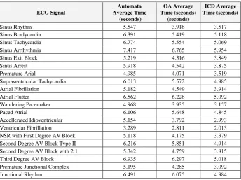
We test 200 signals that are multiple ECG patternsand repeat the test 5 times. In computer programming, we are developing with the C++ language. Experiment results in Table 3-4.

Table 3. Signal Idenify Recognition

ECG Signal

Automata Average Time

(seconds)

OA Average Time (seconds)

(seconds)

ICD Average Time (seconds)

Sinus Rhythm 5.547 3.918 3.517

Sinus Bradycardia 6.391 5.419 5.118

Sinus Tachycardia 6.774 5.554 5.069

Sinus Arrthythmia 7.417 6.765 5.954

Sinus Exit Block 5.219 4.316 3.849

Sinus Arrest 5.918 4.542 3.875

Premature Arial 4.985 4.071 3.519

Supraventricular Tachycardia 6.013 5.572 4.985

Atrial Fibrillation 5.182 4.549 3.914

Atrial Flutter 6.562 6.228 5.092

Wandering Pacemaker 4.968 3.935 3.157

Paced Atrial 6.106 5.648 4.845

Accellerated Idioventricular 5.154 3.792 2.993

Ventricular Fibrillation 3.289 2.811 2.013

NSR with First Degree AV Block 5.118 4.175 3.379

Second Degree AV Block Type II 6.216 5.851 4.914

Second Degree AV Block with 2:1 5.342 4.759 3.815

Third Degree AV Block 6.935 6.297 5.018

Premature Junctional Complex 5.195 4.285 3.092

Junctional Rhythm 6.491 6.075 4.984

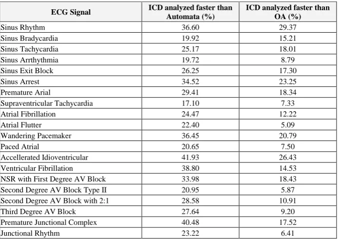
Table 4. Average Percentage of Analyzed

ECG Signal ICD analyzed faster than

Automata (%)

ICD analyzed faster than OA (%)

Sinus Rhythm 36.60 29.37

Sinus Bradycardia 19.92 15.21

Sinus Tachycardia 25.17 18.01

Sinus Arrthythmia 19.72 8.79

Sinus Exit Block 26.25 17.30

Sinus Arrest 34.52 23.25

Premature Arial 29.41 18.34

Supraventricular Tachycardia 17.10 7.33

Atrial Fibrillation 24.47 12.22

Atrial Flutter 22.40 5.09

Wandering Pacemaker 36.45 20.79

Paced Atrial 20.65 7.50

Accellerated Idioventricular 41.93 26.43

Ventricular Fibrillation 38.80 14.53

NSR with First Degree AV Block 33.98 18.43

Second Degree AV Block Type II 20.95 5.87

Second Degree AV Block with 2:1 28.58 10.91

Third Degree AV Block 27.64 9.20

Premature Junctional Complex 40.48 17.52

Junctional Rhythm 23.22 6.41

The study would measure the 200 signals from different ECG signals. Integration Component Diagnosis (ICD) is capable of an unusual accuracy of recognition than the Automata Matching Process 17.10-41.93 average percentage and spends less time than the other 29.37 average percentage method and can alert within 12 seconds period. It cannot be detected in a pattern that is different from without an ECG signal being rec-ognized. The signal is used in the experiment to recognize 20 patterns of the ECG sig-nal. (Figure 3)

5

Conclusion

The Electronic Sensor Kit includes support for a wide range of signal conversion panels, an extensive signal processing algorithm library including Integration Compo-nent Diagnosis (ICD), Optimization Algorithm (OA), convolution, low/high-pass [11], and bandpass filters, and a novelty platform. Although our review has a limited scope, ECG analysis remains an area of intense research. It could be argued. In recent decades, methodologies for pattern recognition have been widely used in this field. While sig-nificant attempts have been and are currently being made to identify the best character-istics suited to the various applications, the emerging device of human identity has not yet achieved a defined status and it is expected that further research by the scientific community will be oriented towards this area.

6

Acknowledgement

This research was supported by Chandrakasem Rajabhat University. Thanks, our colleagues from Chandrakasem Rajabhat University who provided insight and exper-tise that greatly assisted the research.

7

References

[1]Abubakar Adam, Adamu Abubakar, Murni Mahmud. (2019). Sensor Enhanced Health In-formation Systems: Issues and Challenges. International Journal of Interactive Mobile Tech-nologies, Vol 13, No 01, Pages 99-114. https://doi.org/10.3991/ijim.v13i01.7037

[2] Ahilan Appathurai, J. Jerusalin Carol, C. Raja, S. N. Kumar, Sujatha Krishnamoorthy. (2019). A study on ECG signal characterization and practical implementation of some ECG characterization techniques. Measurement, Volume 147, December 2019, Article 106384. https://doi.org/10.1016/j.measurement.2019.02.040

[3]Anchana Muankid, Mahasak Ketcham. (2019). The Real-time Electrocardiogram Signal Monitoring System in Wireless Sensor Network. International Journal of Online and Bio-medical Engineering, Vol 15, No 02, Pages 4-20. https://doi.org/10.3991/ijoe.v15i02.9422 [4]Anthony G. Pompa, Peter LaRossa, Lee B. Beerman, Yoshimi Sogawa, Gaurav Arora.

(2019). Utility of ECGs in the pediatric emergency department for patients presenting with a seizure. The American Journal of Emergency Medicine. Available online 20 November 2019. https://doi.org/10.1016/j.ajem.2019.11.016

[5]Aykut Diker, Engin Avci, Erkan Tanyildizi, Mehmet Gedikpinar. (2019). A Novel ECG Signal Classification Method using DEA-ELM. Medical Hypotheses, In press, journal pre-proof, Available online 13 December 2019, Article 109515. https://doi.org/10.1016/j. mehy.2019.109515

[6]Carmen Camara, Pedro Peris-Lopez, Lorena Gonzalez-Manzano, Juan Tapiador. Real-time electrocardiogram streams for continuous authentication. Applied Soft Computing, Volume 68, July 2018, Pages 784-794. https://doi.org/10.1016/j.asoc.2017.07.032

[8]Emrah Bozbeyoğlu, Emre Aslanger, Özlem Yıldırımtürk, Barış Şimşek, Muzaffer Değerte-kin. (2018). An algorithm for the differentiation of the infarct territory in difficult to discern electrocardiograms. Journal of Electrocardiology, Volume 51, Issue 6, November–Decem-ber 2018, Pages 1055-1060. https://doi.org/10.1016/j.jelectrocard.2018.09.006

[9]Gherardo Finocchiaro, Nabeel Sheikh, Elena Biagini, Michael Papadakis, Iacopo Olivotto. (2019). The electrocardiogram in the diagnosis and management of patients with hyper-trophic cardiomyopathy. Heart Rhythm, In press, corrected proof, Available online 10 Au-gust 2019. https://doi.org/10.1016/j.hrthm.2019.07.019

[10]Henry J. Lin, Yueh-Tze Lan, Michael J. Silka, Nancy J. Halnon, Ruey-Kang Chang. Home use of a compact, 12‑lead ECG recording system for newborns. Journal of Electrocardiol-ogy, Volume 53, March–April 2019, Pages 89-94. https://doi.org/10.1016/j.jelectro-card.2019.01.086

[11]Jonas Isaksen, Remo Leber, Ramun Schmid, Hans-Jakob Schmid, Roger Abächerli. (2017). Quantification of the first-order high-pass filter's influence on the automatic measurements of the electrocardiogram. Computer Methods and Programs in Biomedicine, Volume 139, February 2017, Pages 163-169. https://doi.org/10.1016/j.cmpb.2016.11.003

[12]Kandala N. V. P. S. Rajesh, Ravindra Dhuli. (2017). Classification of ECG heartbeats using nonlinear decomposition methods and support vector machine. Computers in Biology and Medicine, Volume 87, 1 August 2017, Pages 271-284. https://doi.org/10.1016/j.compbio-med.2017.06.006

[13]Luca Mesin. (2017). Heartbeat monitoring from adaptively down-sampled electrocardio-gram. Computers in Biology and Medicine, Volume 84, 1 May 2017, Pages 217-225. https://doi.org/10.1016/j.compbiomed.2017.03.023

[14]M. K. Moridani, M. Abdi Zadeh, Z. Shahiazar Mazraeh. (2019). An Efficient Automated Algorithm for Distinguishing Normal and Abnormal ECG Signal. IRBM, Volume 40, Issue 6, December 2019, Pages 332-340. https://doi.org/10.1016/j.irbm.2019.09.002

[15]Margherita Padeletti, Giuseppe Bagliani, Roberto De Ponti, Fabio M. Leonelli, Emanuela T. Locati. (2019). Surface Electrocardiogram Recording: Baseline 12-lead and Ambulatory Electrocardiogram Monitoring. Cardiac Electrophysiology Clinics, Volume 11, Issue 2, June 2019, Pages 189-201. https://doi.org/10.1016/j.ccep.2019.01.004

[16]Mounaim Aqil, Atman Jbari, Abdennasser Bourouhou. (2017). ECG Signal Denoising by Discrete Wavelet Transform. International Journal of Online and Biomedical Engineering, Vol 13, No 09, Pages 51-68. https://doi.org/10.3991/ijoe.v13i09.7159

[17]Rajani Akula, Hamdi Mohamed. (2019). Automation algorithm to detect and quantify Elec-trocardiogram waves and intervals. Procedia Computer Science, Volume 151, 2019, Pages 941-946. https://doi.org/10.1016/j.procs.2019.04.131

[18]Rajender Singh, Jeremy J. Murphy. (2018). Electrocardiogram and arrhythmias. Anaesthesia & Intensive Care Medicine, Volume 19, Issue 6, June 2018, Pages 322-325. https://doi.org/10.1016/j.mpaic.2018.03.014

[19]S. Kota, C. B. Swisher, T. Al-Shargabi, N. Andescavage, R. B. Govindan. (2017). Identifi-cation of QRS complex in non-stationary electrocardiogram of sick infants. Computers in Biology and Medicine, Volume 87, 1 August 2017, Pages 211-216. https://doi.org/10.1016 /j.compbiomed.2017.05.033

[20]Safri, Wan Nishfa Dewi, Erwin. (2018). Analysis of electrocardiogram recording lead II in patients with cardiovascular disease. Enfermería Clínica, Volume 29, Supplement 1, March 2019, Pages 23-25. https://doi.org/10.1016/j.enfcli.2018.11.011

[22]Teresa Rocha, Simão Paredes, Ramona Cabiddu, Ricardo Couceiro, Paulo Carvalho, Jorge Henriques. (2019). A Tool for ECG Analysis as a Module of a Tele-Monitoring System. International Journal of Online and Biomedical Engineering, Vol 13, No 09, Pages 64-67. http://dx.doi.org/10.3991/ijoe.v12i04.5260. https://doi.org/10.1109/expat.2015.7463235 [23]Tomas Novotny, Raymond Bond, Irena Andrsova, Lumir Koc, Marek Malik. (2017). The

role of computerized diagnostic proposals in the interpretation of the 12-lead electrocardio-gram by cardiology and non-cardiology fellows. International Journal of Medical Informat-ics, Volume 101, May 2017, Pages 85-92. https://doi.org/10.1016/j.ijmedinf.2017.02.007 [24]Weiyi Yang, Yujuan Si, Di Wang, Gong Zhang. (2019). A Novel Method for Identifying

Electrocardiograms Using an Independent Component Analysis and Principal Component Analysis Network. Measurement, In press, journal pre-proof, Available online 5 December 2019, Article 107363. https://doi.org/10.1016/j.measurement.2019.107363

8

Author

Kittimasak Naijit works as a lecturer in Multimedia Technology, Faculty of Science at Chandrakasem Rajabhat University, Bangkok, Thailand, 10900. He has got the bach-elor’s 2 degrees in Computer Education and Computer Engineering, and graduated with a master’s degree in Computer Technology, King Mongkut's University of Technology North Bangkok (KMUTNB). His research interests are in the area of artificial intelli-gence, robotics, information technology systems and multimedia technology.