The Genomic Standards Consortium
Standard operating procedure for computing
pangenome trees
Lars Snipen1,2* and David W. Ussery2
1 Biostatistics, Department of Chemistry, Biotechnology and Food Science, Norwegian University of Life Sciences, Ås, Norway
2 Center for Biological Sequence Analysis, Technical University of Denmark, Lyngby, Denmark
*Corresponding author: Lars Snipen
We present the pan-genome tree as a tool for visualizing similarities and differences between closely related microbial genomes within a species or genus. Distance between genomes is computed as a weighted relative Manhattan distance based on gene family presence/absence. The weights can be chosen with emphasis on groups of gene families conserved to various degrees inside the pan-genome. The software is available for free as an R-package.
Introduction
Currently, there are about a thousand sequenced prokaryotic genomes in GenBank, and several thousand more are in various stages of comple-tion. For many bacterial species, sequenced ge-nomes from several different strains are available, opening the possibility to study pan-genomes or supra-genomes. The pan-genome of a species or genus, as opposed to the genome of a single strain, is defined as the union of all gene families found at least once in a genome within that species or ge-nus [1,2]. Studying the diversity within pan-genomes is of interest for the characterization of the species or genus. Low pan-genome diversity could be reflective of a stable environment, while bacterial species with substantial abilities to adapt to various environments would be expected to have high pan-genome diversity. Visualizing the relations between genomes within pan-genomes could also be helpful in establishing a picture of the degree of horizontal gene transfer (HGT), as well as aid in the understanding of phenotypic differences.
Diversity between genomes is often displayed in the form of trees. Over the past decade several procedures have been proposed for constructing trees from more or less whole-genome data [3,4]. Many strategies have been employed, and two major approaches are sequence-based and gene-content based trees. Sequence based trees include
super-trees and phylogenomic trees, and their construction is based more or less directly on se-quence alignments and evolutionary distances known from classical phylogenetics [5-7]. The gene content trees use as data the pres-ence/absence of genes in the various genomes, and compute distance between genomes from such data [8,9]. The pan-genome tree described here would naturally be categorized amongst the gene-content trees.
functional relationship between a “snapshot” set of sequenced genomes.
Requirements
The software is implemented in R, which is a freely available computing environment, see
pan-genomics is under construction, and a pre-release version is available upon request from the corresponding author. The computation of gene families mentioned in this paper is based on BLAST,
which is available
Procedure
Gene families
Sequences are grouped into gene families based on sequence similarity. A FASTA formatted file with all protein sequences for one genome is BLASTed against similar sequences for all ge-nomes, including itself. Two sequences are in the same gene family if there are significant align-ments between them when either sequence is used as query, and when both these alignments span at least 50% of the length of the query se-quence and contain at least 50% identity ([1]). The gene family results are represented in a pan-matrix M, where each row corresponds to a
ge-nome and each column to a gene family. Element
Mi,j is 1 if gene family j is present in genome i, or 0 if not. Hence, each row of M is a sequence of
bi-nary digits which we refer to as the pan-genome profile of the corresponding genome. When we use the term “genes” below we actually mean gene families.
Pan-genome trees
The genome trees are formed on the basis of dis-tance between pan-genome profiles. We use a relative Manhattan distance, i.e. the distance
between genome i and k is
( )
, , ,
1
1
n|
|
i k j i j k j j
D
w
M
M
W
=
=
∑
−
where n is the total number of gene families, wj is some gene family specific weight and W is the sum
of these weights. As default wj=1 for all j, but some genes may be down-weighted, as described below. This distance describes the proportion of the pan-genome in which pan-genome i and k differ. A
fre-quently used distance for phylogenetic gene-content trees is the Jaccard distance [10].
Consi-dering genomes A and B, genes are either i) present in both, ii) present in A and absent in B, iii) absent in A and present in B or iv) absent in both. The Jaccard distance is 1 minus the number of genes in class i) divided by the sum of genes in class ii) and iii). The Manhattan distance we use above is the sum of genes in ii) and iii) divided by the sum of all genes. A similar, unweighted, dis-tance was also used in [11] in their construction of the pan-genome tree.
Using this distance measure, trees can be formed by hierarchical clustering. We have employed an average linkage, corresponding to the Unweighted Pair-Group Method with Arithmetic mean (UPG-MA) algorithm; UPGMA has been previously used in the building of phylogenetic trees.
Bootstrapping is frequently used to illustrate the stability of the branching in a tree. We have im-plemented this by re-sampling gene families, i.e.
columns of the pan-matrix, and re-clustering these data. The bootstrap-value for a split is the percen-tage of the re-sampled trees having a similar node, i.e. with the same two sets of leaves in the branches.
Gene family weights
The core genes, i.e. the gene families present in all
genomes, contribute to no difference between genomes, and could be discarded, i.e. given weight
zero. Other gene families may also be down-weighted. Genes found in only one single genome, referred to as ORFans, are often dubious and can be the product of over-sensitive gene finders. Hence, giving such genes zero weight could im-prove the robustness of the tree to these types of errors.
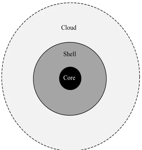
It has been observed that genes could be divided into classes depending on their degree of conser-vation within the pan-genome. This is the basis for the use of mixture models to predict pan-genome size [12,13]. In [14] the bacterial pan-genome was divided into three major categories, core, shell and cloud, as illustrated in Figure 1.
ecological niches. For example, the shell and cloud would be expected to be larger for Actinobacteria
and other organisms that produce secondary me-tabolites. Further, the pan-genomes of phyla could contain specific pathways which are phy-lum- or class-specific (e.g. polyketides type I and II
pathways, aminoglycosides, non-ribosomal pep-tides, β-lactams, etc), that would be part of phylum
specific shells. On the other hand, pathogenic, parasitic and commensal species that are not rou-tinely found in the environment could have small-er clouds.
Figure 1. The bacterial pan-genome can be divided into the core (genes always occurring in any genome inside the pan-genome) the shell (genes frequently occurring) and cloud (rarely occurring genes).
Implementation
Standard settings for BLASTp were used, except the E-value cutoff, where we use 10-5. A more
lib-eral cutoff will have very small effects on the final results, but will slow down the procedure signifi-cantly by producing a lot of poorer alignments in addition to the best alignments. Since the BLAST-ing and parsBLAST-ing of BLAST results is the computa-tional bottleneck of this procedure we have found this cutoff appropriate. The remaining computa-tions and plotting have been implemented in R as part of a package for microbial pan-genomics.
Pan-genome tree versus 16S phylogenetic tree
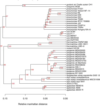
Figure 3 show a pan-genome family tree for the genus Streptococcus, based on 42 completed
ge-nomes downloaded from NCBI in August 2009. We have used this genus as an example, because it contains several species with multiple completed genomes. All genomes within each species cluster together, without exception, and further the reso-lution is good enough to distinguish smaller dif-ferences among strains within the species.
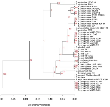
In Figure 4 we have, for comparison to Figure 3, included another tree for the same genus, based on the more traditional approach of computing evolutionary distances from the multiple align-ment of the 16S ribosomal RNA sequences of each genome. Here we typically see extremely small distances between many strains, combined with some bigger distances, giving a lower resolution. Also, S. pyogenes is divided into two very different
clusters with 7 and 5 genomes in each. The small-er clustsmall-er of S. pyogenes strains all share an almost
identical annotation of the 16S sequences differing in length from all other streptococci. In the pan-genome tree of Figure 3 this division of S. pyogenes
strains is not supported. Also the S. agalactiae
genomes are no longer clustered in the 16S tree, and the strain S. pneumoniae R6 is also found
se-parated from all other S. pneumoniae strains. The
16S tree was constructed using UPGMA in order to make it comparable to that in Figure 3. UPGMA is in general not accepted as a proper way of re-constructing phylogenetic trees, but a tree built by neighbor-joining verified the separation of strains, even if distances between nodes changed (not shown).
Effect of weights
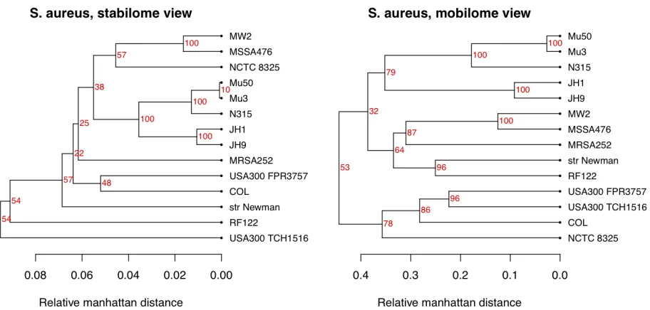
In Figure 5 we illustrate different choices of weights. Here we have used data for a single spe-cies, Staphylococcus aureus. Annotated proteins
for all completed genomes of this species were downloaded from NCBI. Note that there are some differences in clustering - for example, the two USA300 strains, which are community-acquired methicillin-resistant strains [15] that would be expected to be similar, are not as close in the shell, but cluster together when more weight is given to the “cloudy part” of the pan-genome. Thus, these two strains are not very similar when we consider the S. aureus typical part of the genomes, but
Figure 2. The left panel shows as an example the number of gene families found in 1, 2,…,14 genomes of the 14 completed genomes of Staphylococcus aureus downloaded from NCBI in July 2009. The right panel illustrates three possible weighting schemes. The green bars give weight 1.0 to all gene families except the ORFans, i.e. those gene families only present in one genome, who get weight 0.0 (discarded). The blue bars give a gradually higher weight to the gene families found in the majority of the genomes, the shell. The red bars illustrate the opposite strategy, emphasizing the cloud. All gene families found in the same number of genomes get the same weights.
Discussion
We present here the pan-genome tree as a stan-dard operating procedure in the pan-genomic toolbox. It is a whole-genome tree not unlike many other gene-content trees, but with the emphasis on describing functional differences between closely related genomes, within a species or genus. Examples of successful use of variants of such trees are [11] and [16].
The distance between genomes is the relative Manhattan distance between pan-genome profiles. Two genomes are similar not only by sharing the same genes as defined by the Jaccard distance, but also by lacking the same genes. The latter is mea-ningful inside a pan-genome where all the genes could in principle be present. When looking for differences in phenotype those parts of the
“ma-chinery” which are absent are just as important as those that are present. In [17] an estimate of shared absence was introduced by including a third reference genome when comparing two ge-nomes of interest. In our case the pan-genome plays the role as the reference genome.
The weights illustrated in Figure 2 are only a se-lection out of a long range of possible choices. Dis-carding ORFans, and emphasizing the shell or cloud, are, however, strategies with a meaning. Weighted distances in gene-content trees have been used before, e.g. [18]. Two of their weighting
strategies, termed prevalence-weighted and rari-ty-weighted trees, are in principle similar to what we call shell and cloud strategies.
Figure 5. The left panel show the pan-genome family tree for the 14 strains of Staphylococcus aureus
completed as NCBI. Here the weights have been chosen according to the blue bars in Figure 1, i.e. the “stabilome” genes have been emphasized. In the right panel, the same data have been used, but weights are now chosen to emphasize the “mobilome” genes. In both cases ORFans have been discarded.
A pan-genome profile of a genome is a vector of 1s (present) and 0s (absent) with N elements if the pan-genome has N gene families. In [10] the term conservation profile was used for a similar vector, but with one vector for each gene sequence in each genome. Merging these sequence-specific conservation profiles into one pan-genome profile for the entire genome is in principle what is done when gene families are computed and the pan-matrix constructed. We compute gene families in a simple way, using BLAST and a simple cutoff-rule. This will have to change in the near future, because the alignment of all-against-all is not a
computationally feasible solution as the number of genomes grows. Computing gene families by BLASTing against a database like COG [19] has been a common strategy and Wolf et al. [8]
con-cluded that gene-content trees based on pres-ence/absence of such gene families resulted in a grouping of genomes based on phenotype. How-ever, groups of orthologs, like the COGs, are often large and diverse and in our experience give too few and too large gene families to achieve good resolution when clustering closely related ge-nomes. We are currently working on improve-ments of this.
References
1. Tettelin H, Masignani V, Cieslewicz MJ, Donati C, Medini D, Ward NL, Angiuoli SV, Crabtree J, Jones AJ, Durkin AS, et al. Genome analysis of multiple pathogenic isolates of Streptococcus aga-lactiae: implications for the microbial pan-genome. . Proc Natl Acad Sci USA 2005; 102: 13950-13955
2. Medini D, Donati C, Tettelin H, Masignani V, Rappuoli R. The microbial pan-genome. Curr Opin Genet Dev 2005; 15: 589-594
3. Snel B, Bork P, Huynen MA. Genome phylogeny base don gene content. Nat Genet 1999; 21:
108-110
4. Snel B, Huynen MA, Dutilh BE. Genome trees and the nature of genome evolution. Annu Rev Microbiol 2005; 59: 191-209
5. Brown JR, Douady CJ, Italia MJ, Marshall WE, Stanhope MJ. Universal trees based on large combined protein sequence data sets. Nat Genet
2001; 28: 281-285
in molecular phylogeneties. Nature 2003; 425:
798-804
7. Wu M, Eisen JA. A simple, fast, and accurate me-thod of phylogenomic inference. Genome Biol
2008; 9: R151
8. Wolf YI, Rogozin IB, Grishin NV, Tatusov RL, Koonin EV. Genome trees constructed using five different approaches suggest new major bacterial clades. BMC Evolutionary Biology 2001; 1: 8
9. Gu X, Zhang H. Genome phylogenetic analysis based on extended gene contents. Mol Biol Evol
2004; 21: 1401-1408
10. Tekaia F, Yeramian E. Genome trees from conservation profiles. PLoS Computational Biology 2005; 1:e75.
11. Hiller NL, Janto B, Hogg JS, Boissy R, Yu S, Pow-ell E, Keefe R, Ehrlich NE, Shen K, Hayes J, et al. Comparative Genomic Analyses of Seventeen
Streptococcus pneumoniae strains: Insight into the Pneumococcal Supragenome. J Bacteriol
2007; 189: 8186-8195
12. Hogg JS, Hu FZ, Janto B, Boissy R, Hayes J, Keefe R, Post JC, Erlich GD. Characterization and mod-elling of the Haemophilus influenzae core- and supra-genomes based on the complete genomic sequences of Rd and 12 clinical nontypeable strains. Genome Biology 2007; 8: R103
13. Snipen L, Almøy T, Ussery DW. Microbial com-parative pan-genomics using binomial mixture models. BMC Genomics 2009; 10: 385
doi:10.1186/1471-2164-10-385
14. Koonin EV, Wolf YI. Genomics of Bacteria and
Archaea: the emerging dynamic view of the pro-karyotic world. Nucleic Acids Res 2008; 36:
6688-6719
15. Diep BA, Gill SR, Chang RF, Phan THV, Chen JH, Davidson MG, Lin F, Lin J, Carleton HA,
Mongodin EF, et al. Complete genome sequence of USA300, an epidemic clone of community-acquired meticillin-resistant Staphylococcus aureus. Lancet 2006; 367: 731-739
16. Vesth T, Wassenaar T, Hallin P, Snipen L, Lagesen K, Ussery DW. On the origins of a Vibrio species. Microbial Ecology. 59:1-
17. McCann A, Cotton JA, McInerney JO. The tree of genomes: An empirical comparison of genome-phylogeny reconstruction methods. BMC Evol. Biol. 2008, 8:312
18. Gophna U, Doolittle WF, Charlebois RL. Weighted Genome Trees: Refinements and Applications. J Bacteriol 2005; 187: 1305-1316
19. Tatusov RL, Fedorova ND, Jackson JD, Jacobs AR, Kiryutin B, Koonin EV, Krylov DM, Mazumder R, Mekhedov SL, Nikolskaya AN, et al. The COG database: an updated version includes eukaryotes.
BMC Bioinformatics 2003; 4: 41