Application of wireless technologies to forward predict crop yields in the poultry production chain

Application of wireless technologies to forward predict crop

yields in the poultry production chain

Patrick Jackman

_{, Shane Ward}

_{, Liam Brennan}

_{, Gerard Corkery}

and Ultan McCarthy

(1. Biosystems Engineering, University College Dublin, Belfield, Dublin, Ireland; 2.Department of Applied Sciences, Dundalk Institute of Technology, Louth, Ireland; 3.Intelligent Mechatronics and RFID Gateway, Tralee Institute of Technology, Kerry, Ireland.)

Abstract: Average bird weight is the primary measure of crop yield and is the basis for calculating payment for the grower by the wholesaler. Furthermore the profit per bird is very small. Thus very tight control of growing process that is essential to ensure average bird weight is maximised. The important factors (air temperature, air humidity, carbon dioxide concentration and ammonia concentration) that affect the intake of feed and water must be kept at their optimum during the progress of the growing cycle. These factors can be influenced by activating burners and opening the vents on walls of the growing house. It then follows that the burning and venting strategy will be influential on the average bird weight of the crop.

Currently the burning and venting strategy is based on notional ideal levels and data from wall mounted sensors. This suffers from two fundamental problems: firstly the strategy is determined by ideals that may not be suitable for all growing houses and secondly the data are not measured from the chickens own airspace. Thus the management strategy is based on a model that may not reflect reality and on data that may not reflect reality

The “BOSCA” project addresses these problems by placing wireless environmental sensors into the chickens own airspace. This provides for direct measurement of the air experienced by the chickens and reports the recorded data in near real-time to a cloud based data management system. The sensor data are merged with the data from the growing house weighing scales in the cloud repository so a predictive model of average bird weight from the measured environmental data can be calibrated and validated. Furthermore, a time shift can be applied to the environmental data during model calibration and validation so the average bird weight can be forward predicted by 72 h(R2up to 0.89 with neural networks). This gives the grower advance notice of a deviation from ideal feeding and watering conditions and the likely consequences of failing to take remedial action such as turning on the burners or venting the house.

Keywords: environmental control, productivity, average bird weight, wireless agricultural sensors, cloud computing

Citation: Jackman, P., S. Ward, L. Brennan, G. Corkery, and U. McCarthy. 2015. Application of wireless technologies to forward predict crop yields in the poultry production chain. Agric Eng Int: CIGR Journal, 17(2):287-295.

1 Introduction

It is anticipated that there will be very strong growth

in the global poultry market into the next decade (Mulder,

2012), thus it is essential that anyone wishing to maintain

or grow their market share will have adopt the best

standards and practices. Specifically it will be necessary

for producers to maximise their average bird weights by

maintaining high feed and water conversion efficiencies

Received date: 2014-09-23 Accepted date:2015-04-08

*Corresponding author: Patrick Jackman. Biosystems Engineering, University College Dublin, Belfield, Dublin, Ireland. Email: [email protected]

throughout the production cycle (Van Horne and Bondt,

2013).It should be noted that in a typical production cycle

(five to six week period) average bird weights can

increase from 50 g to 2.2 kg(Hall and Sandilands, 2007).

The comfort and the contentment of the broiler

chickens depend on the control of the house environment.

More specifically this means that the air temperature,

humidity, carbon dioxide (CO2) and ammonia (NH3) must

be within acceptable parameters (Aviagen, 2009). These

parameters can be maintained by an in-house

environmental control system (Rotem, 2014) which

controlling the use of heaters, air conditioning and

external vents and other environmental manipulation

devices. However, burners that use gas or liquid diesel

fuel to generate additional heat at the cost of also

introducing additional CO2 into the house environment.

The gas concentrations and importantly the house

temperature and humidity can be lowered by opening

vents on the walls of the house to allow fresh air to enter

the house and stale air to escape (Aviagen, 2009).

However, venting due to excessive gas concentrations or

humidity may mean that the heaters need to be activated

to maintain temperature.

In addition to the economic requirements for close

control of poultry house environments there is a legal

requirement in respect of animal welfare and workers

healthcare (Corkery et al., 2013) and it is insufficient to

merely reduce flock density to guarantee animal welfare

(Jones et al., 2005) so additional welfare supports

arerequired. The trend in regulation is towards

progressively stricter limits on the house environment but

equally the grower does not want use the environmental

manipulation mechanisms as they are costly to use

(Jones-Hamilton, 2014). Thus, the solution is the

optimum use of the environmental manipulation

mechanisms, which is a type of Precision Livestock

Farming (PLF), towards a reduction in production losses

(Mollo et al., 2009) leading to better incomes, reduced

environmental impact, increased product quality, earlier

diagnosis of health risks and improved waste

management (Hocquette and Chatellier, 2011). The

principal characteristics of good PLF systems are

continuous adequate sensing, dynamic mathematical

models, target values for outputs and model based

predictive controllers (Wathes et al., 2008).

To implement a PLF solution, poultry growers

typically install an automatic environmental control

system which uses standard curves and the growers’

inputs to make process decisions. However, these systems

suffer from a number of shortcomings in that they use

mounted sensors and thus they are not in direct contact

with the chickens own airspace. Hence, the

environmental control algorithms must make their

decisions based on data that may be unrepresentative.

Similarly the decision making algorithms are generic may

not be appropriate to the unique characteristics of the

particular growing house.Another weakness is that there

is no cloud sharing of data meaning the data is only

available locally.

Thus, there is an industry gap for a new PLF solution

for poultry houses that can avail of data directly measured

from the chickens own airspace so decisions can be made

based on truly representative data. There is a further gap

in using decision algorithms that are tailored to the

uniqueness of the growing house in question that can be

quickly calibrated and validated from a small number of

training crops.

In particular what be of great value would be a

predictive facility that could estimate the likely impact of

a loss of environmental control or a failure to maintain

optimum environmental conditions. This would be an

advance on the traditional predictive models of bird

weight that estimate future weights based on past weights

during that crop cycle. Thus such an environmental model

could be optimised on a house by house basis after a

period of training and testing. The traditional bird weight

gain models do not have this capacity for optimisation

nor do they have the ability to incorporate environmental

data into their predictions.

The decision making algorithms must have a

substantial forward prediction capability so there is

enough time to take remedial action before the problem

becomes irrecoverable. Furthermore the longer the

forward prediction period the better as there is more time

for a manual intervention by the grower if required. The

sharing of all of this data on a cloud platform will greatly

enhance its usefulness as all interested parties will be able

to benefit including the wholesaler, the retailer and the

2 Materials and methods

2.1 BOSCA design

Bespoke environmental sensing boxes suitable for use

in poultry houses (each known as a “BOSCA”) were

constructed by Shimmer Sensing (Dublin, Ireland); these

consisted of a robust box design, sensors, a sensor board,

a Raspberry Pi and a 3G communication device. The

BOSCAs were programmed with appropriate firmware

and software to record readings as comma separated

values and to allow transmission over the 3G network.

The environmental sensors chosen for suitability for the

task were: a Sensirion (London, United Kingdom) SHT21

temperature and humidity sensor, an Elektronik (Bremen,

Germany) EE891 carbon dioxide sensor and a Winsensor

(Zhengzhou, China) MQ137 ammonia sensor. Two

variants of the sensor boxes were constructed; a “BOSCA-MOR” or big box which contains all the elements described and a “BOSCA-BEAG” or small box

which does not contain gas sensors and a 3G

communication device. The BOSCA-BEAGs

communicated their data to any BOSCA-MORs within

range.

Calibration experiments were performed to verify the

calibration curves that were embedded in the BOSCA

firmware. The sensor boxes were placed into a culture

cabinet (Binder, Tuttlingen, Germany) where

temperature, humidity and gas concentrations could be

manipulated. Inside the cabinet were a Davis Vantage

Pro2 weather station (Davis, Hayward, California, USA)

and a Geotech G100 CO2 gas detector (Geotech,

Leamington Spa, United Kingdom). Special NH3 rich air

was supplied by BOC gases (Dublin, Ireland) at 25mg/kg

and 50 mg/kg. As a result some adjustments to the

BOSCA firmware were required to edit the calibration

polynomials.

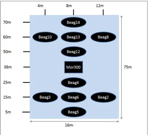
2.2 BOSCA deployments

The BOSCAs were deployed in a growing house in

County Monaghan, Ireland for two crop cycles. The

schematics are shown in Figures 1 and 2. Each BOSCA

was placed in this location for the full cycle. The data

recorded were condensed into comma separated values

(.csv) every 1 min for the BOSCA-MORs and every 10

min for the BOSCA-BEAGs. The .csv files were

immediately uploaded to a cloud server via the 3G

connection using a standard file transfer protocol (ftp)

process. A local copy of the sensor data repository was

made on a Linux server in University College Dublin

where the .csv were parsed by bespoke Python and Bash

scripts to facilitate their entry onto a PostgreSQL

database suitable for forensic queries and web portal

interface.

Figure 1Planar schematic of placement of sensor boxes in

Figure 2 Planar schematic of placement of sensor boxes

in the growing house for the second crop cycle

2.3 Data processing

Time series data for each BOSCA and each sensor

within the BOSCAs were extracted from the PostgreSQL

database with standard SQL queries (e.g. SELECT

VALUE from READINGS where SENSOR_ID = …)

with a Python for Linux interface. The time series data

were saved as an excel spreadsheet where it was joined

with the daily average bird weight data provided by the

chicken grower. To make the data comparable all of the

time series were grid interpolated into hourly readings.

The hourly readings were copied into the statistical

software MINITAB (Minitab Inc, Cologne, Germany) for

analysis by partial least squares regression (PLSR) and by

neural networks (NN) in Matlab (The Mathworks, Natick,

Massachusetts, United States of America). Sensor

redundancy analysis was performed and both internal

comparison and cross comparison predictive models of

average bird weight in 72 hours’ time were generated.

3 Results and discussion

3.1 Sensor spatial redundancy

A vital question for sensor deployment is the spatial

density required to capture trends and patterns within the

area of interest. Deploying too high a density is a waste of

resources and could also add error to the data stream,

conversely too low a density will cause potentially

important variability in the area to be missed and

consequently important process control decisions to be

distorted. Redundancy in the time series data can be

estimated by a correlation matrix and by extracting the

eigenvalues from a principal component analysis of the

time series matrix. This was performed for both crops 1

and 2 and the results are shown in Tables 1 and 2. The

correlation matrix shows the linear correlation between

any pair of sensors for temperature and humidity, it also

shows the average cross correlation for each sensor. The

eigenvalues for each matrix is shown alongside the

correlation matrix, this shows how much variance is

explained by each successive principal component. It is

important to note that BOSCA-BEAG8 in crop 1 and

BOSCA-MOR200 in crop 2 only performed

intermittently and their data were thus excluded from

3.2 Sensor type redundancy

The inclusion of an ammonia sensor comes at

significant financial cost and thus if it was possible to

estimate ammonia by other means the financial cost of

the BOSCA-MORs could be substantially reduced.

Experience of the industry is that ammonia levels track

humidity levels as the crop progresses. To test this

hypothesis a PLSR model was built using humidity,

temperature and time elapsed as predictors of humidity.

To account for possible non-linearity squared, cubic and

Table 1Temperature and humidity correlation matrices and eigenvalues for the first crop

Temperaturecorrelation matrix

Mor300 Beag2 Beag3 Beag4 Beag5 Beag6 Beag10 Beag12 Beag13 Beag14 Eigenvalues,%

Mor300 93.0

Beag2 0.905 0.905 3.4

Beag3 0.936 0.96 1.896 1.1

Beag4 0.93 0.929 0.954 2.813 0.8

Beag5 0.882 0.941 0.944 0.905 3.672 0.5 Beag6 0.926 0.975 0.975 0.968 0.957 4.801 0.5 Beag10 0.921 0.906 0.936 0.917 0.862 0.923 5.465 0.3 Beag12 0.941 0.934 0.962 0.959 0.897 0.955 0.948 6.596 0.2 Beag13 0.932 0.882 0.921 0.955 0.844 0.925 0.953 0.962 7.374 0.1 Beag14 0.851 0.884 0.865 0.885 0.804 0.892 0.905 0.9 0.907 7.893 0.1

8.224 7.411 6.557 5.589 4.364 3.695 2.806 1.862 0.907 Humiditycorrelation

matrix Humid Correlation Matrix

Mor300 Beag2 Beag3 Beag4 Beag5 Beag6 Beag10 Beag12 Beag13 Beag14 Eigenvalues-Humid Eigenvalues,%

Mor300 93.4

Beag2 0.937 0.937 2.5

Beag3 0.894 0.945 1.839 1.2

Beag4 0.934 0.964 0.907 2.805 0.8

Beag5 0.899 0.943 0.973 0.901 3.716 0.6 Beag6 0.897 0.944 0.973 0.907 0.98 4.701 0.5 Beag10 0.938 0.95 0.952 0.94 0.947 0.946 5.673 0.3 Beag12 0.924 0.942 0.944 0.957 0.943 0.952 0.962 6.624 0.2 Beag13 0.948 0.952 0.937 0.942 0.939 0.939 0.976 0.957 7.59 0.2 Beag14 0.859 0.869 0.909 0.845 0.92 0.941 0.908 0.909 0.915 8.075 0.1

8.23 7.509 6.595 5.492 4.729 3.778 2.846 1.866 0.915

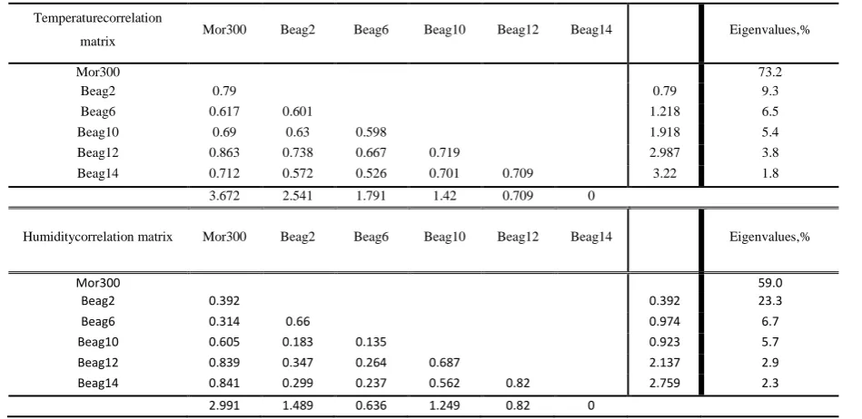
Table 2Temperature and humidity correlation matrices and eigenvalues forthe second crop

Temperaturecorrelation

matrix Mor300 Beag2 Beag6 Beag10 Beag12 Beag14 Eigenvalues,%

Mor300 73.2

Beag2 0.79 0.79 9.3

Beag6 0.617 0.601 1.218 6.5

Beag10 0.69 0.63 0.598 1.918 5.4

Beag12 0.863 0.738 0.667 0.719 2.987 3.8 Beag14 0.712 0.572 0.526 0.701 0.709 3.22 1.8

3.672 2.541 1.791 1.42 0.709 0

Humiditycorrelation matrix Mor300 Beag2 Beag6 Beag10 Beag12 Beag14 Eigenvalues,%

Mor300 59.0

Beag2 0.392 0.392 23.3

Beag6 0.314 0.66 0.974 6.7

Beag10 0.605 0.183 0.135 0.923 5.7

Beag12 0.839 0.347 0.264 0.687 2.137 2.9

Beag14 0.841 0.299 0.237 0.562 0.82 2.759 2.3

interaction terms were included. The PLSR model was

validated by 10-fold cross validation. In parallel a NN

was developed using humidity, temperature and time

elapsed as a predictor of ammonia. The NN was validated

and tested with a 70-15-15 split of the data. The results of

the PLSR predictive models are shown in Figure 3. The

corresponding NN model could on average predict

ammonia with an R2of 0.94.

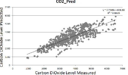
Similarly the inclusion of a carbon dioxide sensor also

comes at noticeable financial cost although less than for

an ammonia sensor and thus its elimination would reduce

the overall costs. As with ammonia, experience within the

industry is that there is a substantial tracking of humidity

levels as the crop progresses. Identical PLSR models and

NN were thus developed to test for redundancy of the

carbon dioxide sensor. The results of the PLSR predictive

models are shown in Figure 4. The corresponding NN

model could on average predict carbon dioxide with an

R2of 0.84.

3.3 Forward predictions of average bird weight

The most useful outcome for a big data would be to

provide an alert system for potential deviations from

weight gain targets for the crop based on parameters that

can be adjusted by the grower. The further into the future

this model could predict the better but industry

experience is that a few days would be adequate. Thus a

72 h time shift was applied to the average bird weight

data so sensor readings were matched to average bird

weight 72 h into the future. The time series were then

used for PLSR and NN modelling in two contexts. The

first was where the data from both crops was merged to

form a single dataset; this would produce a growing

house specific model that may not generalise well in Figure 3 Results of a PLSR model of ammonia level in mg/kgfrom linear, squared, cubic and interaction terms

of humidity, temperature and time elapsed

other growing houses. The second was where a model

calibrated from one dataset was applied on the other and

vice versa, this would produce more conservative results

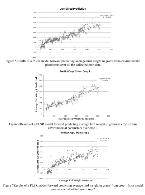
but would generalise better. The PLSR models were

validated by 10-fold cross validation. The PLSR results

are shown in Figures 5, 6and 7. The corresponding NN

models were again validated and tested with a 70-15-15

split of the data. The NN model predictions were R2 =

0.89 for the combined crop dataset, R2 = 0.89 for

forward predicting the crop 2 average bird weight from a

model developed from the crop 1 data and finally R2 =

0.79 for forward predicting the crop 1 average bird

Figure 5Results of a PLSR model forward predicting average bird weight in grams from environmental parameters over all the collected crop data

Figure 6Results of a PLSR model forward predicting average bird weight in grams in crop 2 from environmental parameters over crop 1

weight from a model developed from the crop 2 data.

3.4 Discussion

The key question of sensor spatial redundancy has

been investigated in detail. The spatial arrangement in the

first crop places all BOSCAs in areas that have good air

circulation and are free from major obstructions. Thus it

is no surprise that there is a very strong intra sensor

correlation and very high proportions of variance are

expressed in the first few eigenvalues. This would

support the view that where air can move freely a very

low density of BOSCAs will be adequate to capture the

trends and patterns of air temperature and humidity.

The spatial arrangement in the second crop places

some BOSCAs in the corners of the house where there

would be less free circulation of air and some large

obstructions are present. In this case the intra sensor

correlations were much weaker except for the BOSCAs in

the centre of the house. Similarly the proportion of

variance expressed in the first few eigenvalues is much

smaller. This would support the view that it is essential to

have sensors deployed in the corners of the house to fully

characterise the trends and patterns in the house.

The results for predicting ammonia from the other

environmental parameters and other crop data are

adequate to replace the ammonia sensor in the

BOSCA-MORs and to estimate the ammonia levels in the

BOSCA-BEAGs. Additional gas calibration experiments

to take place in the laboratories of University College

Dublin can further refine the signal produced by the

ammonia sensor to increase the robustness of the

prediction equations.

The results for predicting carbon dioxide from the

other environmental parameters and other crop data

would not be adequate to replace the carbon dioxide

sensor for two main reasons. Firstly the carbon dioxide

sensor will be substantially cheaper than an ammonia

sensor and secondly poultry farmers and poultry house

managers in Ireland place a very high importance on

direct carbon dioxide readings in their experience when

determining the correct moment to open the house vents,

thus any predictive model of carbon dioxide would need

to be extremely accurate to warrant replacement of a

direct carbon dioxide measurement.

The ability to forward predict by 72 hthe average bird

weight based on current environmental data has ranged

from good to excellent. Where the data from both crops

were envisaged as a single dataset an excellent correlation

with measured average bird weight was found. This

would suggest that it is realistic to attempt to build house

specific models of crop progression, these would not be

expected to generalise well and it would be necessary to

carry out similar experiments in each new house.

Where the data from the crops were treated as distinct

the results were mixed, an excellent prediction of the

progression of crop 2 was possible based on a model

developed with the crop 1 data, however the converse

was not the case and it was more difficult to predict the

progression of crop 1 based on a model developed with

the crop 2 data. These models would be more likely to

generalise as they have had to deal with fully external test

data. The mixed results would suggest that it may be too

ambitious to produce generalised models of crop

progression based on environmental data as the

differences between houses may be too difficult to

capture without a vast program of experiments and the

inclusion of house infrastructural features into the

predictive models.

The benefits of artificial intelligence based modelling

approaches are marginal as the NN model prediction

statistics are only a few percent at best beyond the

classical multivariate statistical model predictions. As

such it is recommended to use explicit methods that can

be more clearly understood rather than opaque artificial

intelligence methods.

Further experimental data arebeing collected in the

same chicken growing house and in other chicken

data which can enhance and refine the results found in

this series of experiments. Similarly additional calibration

experiments are being carried out with ammonia rich gas

mixtures to further refine the ammonia sensor signal.

4 Conclusions

A comprehensive series of experimental work has

been carried out to collect environmental data from a

typical chicken growing house in Ireland. Key questions

of sensor spatial deployment and which sensors are

necessary to characterise the trends and patterns in the

house that lead to weight gain in the crop have been

substantially addressed. Important questions of how

current environmental data can be used to forward predict

crop weight gain have been explored and it has been

proven possible to build a house specific predictive model

that can forecast a few days into the future giving the

grower enough time to take mitigating action.

ACKNOWLEDGEMENTS

This research was carried out with funding from

Science Foundation Ireland and with the support of

Carton Group PLC

References

Aviagen.2009. Ross Broiler Management Manual, Aviagen Group, Huntsville, AL, USA.

Corkery, G., S.Ward, C.Kenny, andP.Hemmingway. 2013. Incorporating Smart Sensing Technologies into the

Poultry Industry. World's Poultry Research, 3(4): 106-128.

Hall, C.,andV.Sandilands. 2007. Public attitudes to the welfare of broiler chickens. Animal Welfare, 16(3): 499-512. Hocquette, J.F.,andV.Chatellier. 2011. Prospects for the European

beef sector over the next 30 years. Animal Frontiers, 1(1): 20-28.

Jones, T.A.,C.A. Donnelly, andM.S.Dawkins. 2005. Environmental and management factors affecting the welfare of chickens on commercial farms in the United Kingdom and Denmark stocked at five densities. Poultry Science, 84(6): 1155-1165.

Jones-Hamilton.2014. Cost Effective Poultry House Ventilation, Jones-Hamilton Agriculture, Walbridge, OH, USA. Mollo, M.N., O.Vendrametto, andM.T.Okano. 2009. Precision

Livestock Tools to Improve Products and Processes in Broiler Production: A Review. Brazilian Journal of Poultry Science, 11(2): 211-218

Mulder, N.-D.2012. Outlook for the Global, European and Irish poultry industry, Rabobank International, Utrecht, Netherlands.

Rotem.2014. Platinum Plus Controller Manual. Rotem Control and Management. Petach-Tikva, Israel.

Van Horne, P.L.M.,andN.Bondt.2013.Competitiveness of the EU poultry meat sector. Wageningen Press, Wageningen, Netherlands.