Microsoft Excel (Lecture Notes)

(1)

ICT Department

Microsoft Excel Lecture

Notes

(2)

LAB1: INTRODUCTION TO MICROSOFT EXCEL

2

1

Open an Existing Workbook file

Open an existing workbook in Excel 1. Click the File tab, and click Open 2. Select the workbook and click Open Open an existing workbook outside of Excel 1. Open Windows Explorer

2. Right-click the file and click Open

1.1

Difference between a workbook and a worksheet:

Workbook Worksheet

A file with a default file name of Book1

The grid where numbers, text, inserted objects and formulas reside and calculations are performed

2

Entering Data

2.1

Understanding Data Types

Data Types Description Default Alignment

Text Composed of characters that cannot be used in calculations Left-aligned

Numbers Numerical characters that can be used in calculations Right-aligned Dates and

times

A special category of numbers that can be used in

(3)

LAB1: INTRODUCTION TO MICROSOFT EXCEL

3

2.2

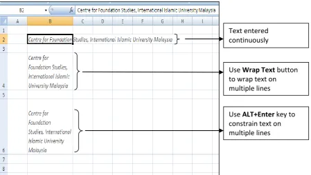
Enter Text

Figure ‎2-1: Text in a cell can cover several cells or be placed on multiple lines.

2.3

Enter numeric data

Enter numbers

1. Click the cell where you want the numbers entered

2. Type the numbers. Use decimal places, thousand separators, and other formatting as you type

Enter numbers using Scientific notation

1. Click the cell where you want the numbers entered 2. Type the number using three components:

 Base: For example: 4, 7.56, -2.5

 Scientific notation identifier: Type the letter “e”

 Exponent: The number of times 10 is multiplied by itself

 For example, scientific notation for the number 123,456,789.0 is written to two decimal places as 1.23 x 108. In Excel you would type 1.23e8

2.4

Enter Dates

Typing‎this‎… Displays this after completing the entry

5/1, 5-1, 1-May or 1-may 1-May

5/1/13, 5-1-13, 5/1/2013, 5-1-2013, 5-1/13 or 5-1/2013 5/1/2013 May 1, 13, May 1, 2013, 1-may-2013 or 1-May-2013 1-May-2013 Note: In cases when a year is omitted, Excel assumes the current year.

Text entered continuously

Use Wrap Text button to wrap text on multiple lines

(4)

LAB1: INTRODUCTION TO MICROSOFT EXCEL

4

3

Editing Data

3.1

Adding data quickly

AutoComplete

Excel will complete an entry for you after you type the first few characters of data that appear in a previous entry in the same column

Auto Fill Auto fill occurs when Excel automatically fills selected cells with data

3.2

Edit cell data

1. Double-click the text in the cell where you want to edit and type the new data.

2. Select the cell to edit, and the click the cell’s contents in the Formula bar and type the new data 3. Select the cell to edit, and press F2. Type the new data

4. Click the cell and type new data.

3.3

Remove cell contents

1. Delete data – Select the cell and press Delete key

2. Move data – Select the cell or range you want to move. Then: i. Place the pointer on any edge of the selection until it turns

into a cross with arrowhead tips. Drag the cell or range to the new location

ii. On the Home tab Clipboard group, click Cut. Select the new location and click Paste in the Clipboard group

(5)

LAB1: INTRODUCTION TO MICROSOFT EXCEL

5

3.4

Copy and Paste Data

Copy data

Select the cells that contain the data you want to copy …

In the Home tab Clipboard group, click the Copy button or click Copy As Picture button

-Or-

Press CTRL+C Paste data

Select the location for the cut or copied data … In the Home tab Clipboard group, click the Paste down arrow and select your option

Right –click the selected cell or range, and on the context menu click Paste Special

and then select your choice.

(6)

LAB1: INTRODUCTION TO MICROSOFT EXCEL

6

3.5

Inserting and Removing Rows, Columns and Cells

Add a single row 1. Select the row below where you want the new row

2. In the Home tab Cells group, click the Insert down arrow, and click Insert Sheet Rows

Add a multiple adjacent rows 1. Select the number of rows below where you want the new rows

2. In the Home tab Cells group, click the Insert down arrow, and click Insert Sheet Rows

Add a single column 1. Select the column to the right of where you want the new column

2. In the Home tab Cells group, click the Insert down arrow, and click Insert Sheet Columns

Add a multiple adjacent columns 1. Select the number of columns to the right of where you want the new column

2. In the Home tab Cells group, click the Insert down arrow, and click Insert Sheet Columns

Add cells 1. Select the cells adjacent to where you want to insert new cells

2. In the Home tab Cells group, click the Insert down arrow, and click Insert Cells

Remove cells, rows and columns 1. Select the single or adjacent items (cells, rows or columns) you wish to remove

2. In the Home tab Cells group, click the Delete down arrow, and click the command applicable to what you want to remove and click Delete

Merge cells 1. Select the cells you want to combine

2. In the Home tab Alignment group, click the Merge & Center down arrow

3. Click the appropriate tool from the list

3.6

Rename a worksheet

1. Right-click the worksheet tab of the worksheet you want to rename, and click Rename. 2. Type a new worksheet name, and press Enter.

3.7

Color a worksheet tab

(7)

LAB1: INTRODUCTION TO MICROSOFT EXCEL

7

4

Saving and closing a workbook

4.1

Save a Workbook

Save a workbook automatically 1. Click the File tab, click Options, and then click Save 2. Select the following settings:

 Click the Save Files In This Format down arrow, and select the default file format

 Ensure the Save AutoRecover Information Every check box is selected, and click the Minutes spinner

3. Click OK when finished Save a workbook manually Click the File tab, and click Save

-Or-

Click the Save button -Or-

Press CTRL+S

4.2

Close the workbook

1. Click the File tab, and click Close -Or-

(8)

LAB 2: CALCULATIONS IN MICROSOFT EXCEL

8

1

Formulas

1.1

Formulas

Formulas are mathematical equations that combine values and cell references with operators to calculate a result.

Values Actual numbers, for example, 35 and 1120.50 Or logical values, for example, True and False

Cell references Cells whose values are to be used, for example, A5: A10

Operators + (add), - (subtract), * (multiply), / (divide), % (modulo), ^ (exponent) Or logical operators such as > (greater than)

Prebuilt formulas, or functions, that return a value also can be used in formulas.

You create formulas by either entering or referencing values. The character that tells Excel to perform a calculation is the equal sign (=), and it must precede any combination of values, cells references and operators.

1.2

Understanding cell referencing types

A cell reference refers to a cell or a range of cells. It tells Excel where to look for the values or data that we want to use in a formula. It is used in formulas, functions, charts and other Excel commands. Cell reference allows:

 usage of data in different parts of a worksheet in one formula.

 usage of value from one cell in several formulas.

 refer to cells on other worksheets in the same workbook.

Cell Reference Description

Relative references Formula move with cells as cells are copied or moved around a worksheet. Absolute references Do not change cell addresses when you copy or move formulas.

(9)

LAB 2: CALCULATIONS IN MICROSOFT EXCEL

9

1.3

Enter a Formula

1.3.1 Using operators and constant

 Click the cell in which you want to enter the formula

 Type equal sign (=)

 Enter the formula

 Press ENTER

Example 1: formula using values

 Select cell B4, then type as example below:

The result will appear like this:

Example 2: formula using cell references

 Find the summation of cell B3 and B4. The result is at cell B5

 At cell B5, type (=) sign, then click cell B3 then type (+), then click cell B4, press ENTER

(10)

LAB 2: CALCULATIONS IN MICROSOFT EXCEL

10

1.4

Copy Formulas

When you copy formulas, relative referencing is applied. Therefore, cell referencing in a formula will change when you copy the formula, unless you have made a reference absolute.

Copy formulas into adjacent cells 1. Select the cell whose formula you want to copy

2. Point at the fill handle in the lower-right corner of the cell, and drag over the cells where you want the formula copied

Copy formulas into nonadjacent cells

1. Select the cell whose formula you want to copy 2. In the Home tab Clipboard group, click Copy or press

CTRL+C

-Or-

Right-click the cell you want to copy, and click Copy

3. Copy formatting along with the formula by selecting the destination cell. Then, in the Home tab Clipboard group, click Paste and then click the Paste icon

-Or-

Copy just the formula by selecting the destination cell. Then, in the Home tab Clipboard group, click the Paste down arrow, and click the Formulas icon.

(11)

LAB 2: CALCULATIONS IN MICROSOFT EXCEL

11

2

Use Functions in Formulas

Functions are prewritten formulas that you can use to perform specific tasks. Let us look some example on how we can use Microsoft Excel built-in functions.

2.1

Mathematical Functions

Table 1: Mathematical Functions

Function Description

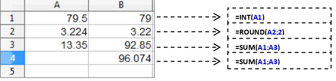
=INT(number) Rounds a number down to the nearest integer. =ROUND(number)

-or-

=ROUND(number, num_digits)

Rounds a number to a specified number of digits.

=SUM(number1; number2; …….. ; number-n)

-or use cell references =SUM(cell1; cell3; cell5) =SUM(cell1:cell5)

Adds all the numbers in a range of cells.

(number1; number2; …….. ; number-n are up to n numbers which sum is to be calculated)

You can also enter a range using cell references.

 Use semicolon (;) to select particulars cells only.

 Use colon (:) to select all cells between the given range.

The sample usage of these mathematical functions is described in Figure 12.12.

Figure XX: Mathematical Functions

=INT(A1)

=ROUND(A2;2)

=SUM(A1:A3)

(12)

LAB 2: CALCULATIONS IN MICROSOFT EXCEL

12

2.2

Statistical Analysis Functions

Table 2: Statistical Analysis Functions

Function Description

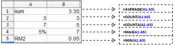
=AVERAGE(number1; number2; …….. ; number30) Retuns the average (text is ignored). =COUNT(number1; number2; …….. ; number30) Counts how many numbers in the list

(text is ignored).

=COUNTA(number1; number2; …….. ; number30) Counts how many values in the list (text is counted too).

=MAX(number1; number2; …….. ; number30) Retuns the maximum value. =MIN(number1; number2; …….. ; number30) Retuns the minimum value.

The sample usage of these statistical analysis functions is described in Figure 12.13.

Figure XX: Statistical Analysis Function

3

Common Errors

###### The column is too narrow to display the complete formatted contents of the cell. #DIV/0! This means you cannot divide zero into a number. For example =A1/A2 would result

#DIV/0! if A2 contains nothing or zero.

#VALUE! Occurs when the wrong type of argument or operand (operand: Items on either side of an operator in a formula. For example, you may have; =A1*A2 and if either cell had text and NOT numbers, the #VALUE! error would be displayed.

#REF! This means a non-valid reference in your formula. Often occurs as the result of deleting rows, columns, cells or Worksheets.

#NAME? This error means a Function used is not being recognized by Excel. Check for typos and always type Excel Functions in lower case.

=AVERAGE(A1:A5)

=COUNT(A1:A5)

=COUNTA(A1:A5)

=MAX(A1:A5)

(13)

LAB 3: FORMATTING & PRINTING IN MICROSOFT EXCEL

13

1

Formatting

1.1

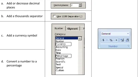
Format numbers

On the Number tab of the Format Cells dialog box, choose the appropriate numeric category (Number, Currency, Accounting, Percentage or Scientific) from the Category list box. Then, select your action:

a. Add or decrease decimal places

b. Add a thousands separator

c. Add a currency symbol

d. Convert a number to a percentage

1.2

Format dates

a. Right-click the cell that contains the date you want to change

Figure ‎1-1: You can choose from among several ways to display dates in Excel

b. Click Format cells on the context menu c. Click the Number tab and then the

Date category

(14)

LAB 3: FORMATTING & PRINTING IN MICROSOFT EXCEL

14

1.3

Change Fonts

1.4

Change Alignment and Orientation

Options available:

 General

 Left (indent)

 Center

 Right (indent)

 Fill

 Justfy

 Center Across Selection

 Distributed

Options available:

 Top

 Center

 Bottom

 Justify

(15)

LAB 3: FORMATTING & PRINTING IN MICROSOFT EXCEL

15

1.5

Change Cell Borders

-or-

(16)

16

1.7

Apply Themes

(17)

17

1.9

Use Format Painter

You can use the Format Painter to quickly apply formatting from text, shapes, and pictures to another text selection, shape, or picture. For example, you can quickly copy a picture border from one picture to another, or copy shape formatting from one shape to multiple shapes.

1. Select the shape, text, or worksheet cell that has the formatting that you want to copy. 2. On the Home tab, in the Clipboard group, click Format Painter.

The pointer changes to a paintbrush.

NOTE: Double-click the Format Painter button if you want to copy the formatting to multiple selections.

3. Select the shape, text, or worksheet cell that has the formatting that you want to format.

To copy the formatting to a single cell, several cells, or a range or ranges of cells, drag the mouse pointer across the cells or ranges of cells that you want to format.

(18)

LAB 3: FORMATTING & PRINTING IN MICROSOFT EXCEL

18

2

Printing

2.1

Add Headers and Footers

1.

2.

(19)

19

2.3

Use Print Areas

You can define a print area of a worksheet by selecting one or more ranges of cells that you want to print.

1. Select the range of cells you want in the print area by dragging from the upper-leftmost cell to the lower-rightmost cell. To include multiple ranges, hold down CTRL while selecting them. 2. In the Page Layout tab Page Setup group, click Print Area and click Set Print Area.

2.4

Display and Print Formula

(20)

20 Print formula:

(21)

LAB 4: CREATING CHARTS IN MICROSOFT EXCEL

21

1

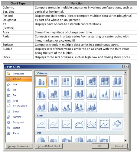
Charts Types

Table below describes each of Excel's chart types. Different charts reflect different kinds of data. If you create one chart and realize it is not the best type of chart to use, you can switch to a different type.

Chart Type Function

Column, Bar, Line

Compare trends in multiple data series in various configurations, such as vertical or horizontal.

Pie and Doughnut

Display one data series (pie) or compare multiple data series (doughnut) as part of a whole or 100 percent.

XY (Scatter)

Displays pairs of data to establish concentrations Area Shows the magnitude of change over time.

Radar Connects changes in a data series from a starting or center point with lines, markers, or a colored fill.

Surface Compares trends in multiple data series in a continuous curve.

Bubble Displays sets of three values similar to an XY chart with the third value being the size of the bubble.

(22)

LAB 4: CREATING CHARTS IN MICROSOFT EXCEL

22

2

Creating a chart

1. Select the data range that you want to chart. 2. In the Insert tab Charts group, click Pie or Column.

2.1

Modify Chart Elements

Task Steps

Add Chart Title

1.

Click the chart

2.

In the Layout tab (Chart Tools) Labels group, click

Chart Title

.

3.

Click one of the options to place the chart title

where you want it

Add Axis Titles (for column chart only)

1.

Click the chart

2.

Axis Titles

.

3.

Point to either the primary horizontal or vertical

axis, and click one of the options to place the

respective axis title where you want it.

Show or Hide Axes (for column chart only)

1.

Click the chart

2.

In the Layout tab (Chart Tools) Axes group, click

Axes

.

3.

Point to:



Primary Horizontal Axis

(or

Vertical Axis

) and

click one of the options to place the axis where

you want it, or click None to remove it.

Add or Remove Gridlines

1.

Click the chart.

2.

In the Layout tab (Chart tools) Axes group, click

Gridlines

.

3.

Point to

Primary Horizontal

(or

Vertical

) Gridlines,

and click one of the options to display major, minor

or both sets of gridlines; or click None to remove

them.

Show or Hide a Legend

1.

Click the chart.

2.

Legend

.

3.

Click one of the options to place the legend where

you want it, or click None to remove it.

Add Data Labels

1.

Click the chart.

2.

Data Labels

.

(23)

LAB 4: CREATING CHARTS IN MICROSOFT EXCEL

23

2.2

Print a Chart

You can print a chart, along with data and other worksheet objects or you can choose to print just the chart, as follows:

1. Select the chart.

2. Click the File tab, and click Print. Under Settings, the Print Selected Chart option is chosen by default.

3. Select a printer and any additional printing options. 4. Click Print when ready.

4% 8%

17%

34% 25%

4% 4% 4%

States of Birth

Perlis Kedah Perak

Selangor Wilayah Persekutuan Melaka

Pahang Sabah

0 1 2 3 4 5 6 7

Level 1 Level 2 Level 3 Level 4 Level 5 Level 6

N o o f Stu d e n ts

English Level

Chart Title Data Labels - Percentage

Legend

Y-axis title X-axis title (Categories)