Generalization Error Bounds in Semi-supervised Classification Under the Cluster Assumption

Generalization Error Bounds in Semi-supervised Classification Under

the Cluster Assumption

Philippe Rigollet [email protected]

School of Mathematics

Georgia Institute of Technology Atlanta, GA 30332-0160, U.S.A

Editor: G´abor Lugosi

Abstract

We consider semi-supervised classification when part of the available data is unlabeled. These unlabeled data can be useful for the classification problem when we make an assumption relating the behavior of the regression function to that of the marginal distribution. Seeger (2000) proposed the well-known cluster assumption as a reasonable one. We propose a mathematical formulation of this assumption and a method based on density level sets estimation that takes advantage of it to achieve fast rates of convergence both in the number of unlabeled examples and the number of labeled examples.

Keywords: semi-supervised learning, statistical learning theory, classification, cluster assumption, generalization bounds

1. Introduction

Semi-supervised classification has been of growing interest over the past few years and many meth-ods have been proposed. The methmeth-ods try to give an answer to the question: “How to improve classification accuracy using unlabeled data together with the labeled data?”. Unlabeled data can be used in different ways depending on the assumptions on the model. There are mainly two ap-proaches to solve this problem. The first one consists in using the unlabeled data to reduce the complexity of the problem in a broad sense. For instance, assume that we have a set of potential classifiers and we want to aggregate them. In that case, unlabeled data is used to measure the com-patibility between the classifiers and reduces the complexity of the set of candidate classifiers (see, for example, Balcan and Blum, 2005; Blum and Mitchell, 1998). Unlabeled data can also be used to reduce the dimension of the problem, which is another way to reduce complexity. For exam-ple, in Belkin and Niyogi (2004), it is assumed that the data actually live on a submanifold of low dimension.

error bounds are available for such methods. In the same spirit, Tipping (1999) and Rattray (2000) propose methods that learn a distance using unlabeled data in order to have intra-cluster distances smaller than inter-clusters distances. The whole family of graph-based methods aims also at using unlabeled data to learn the distances between points. The edges of the graphs reflect the proximity between points. For a detailed survey on graph methods we refer to Zhu (2005). Finally, we mention kernel methods, where unlabeled data are used to build the kernel. Recalling that the kernel measures proximity between points, such methods can also be viewed as learning a distance using unlabeled data (see Bousquet et al., 2004; Chapelle and Zien, 2005; Chapelle et al., 2006).

The cluster assumption can be interpreted in another way, that is, as the requirement that the decision boundary has to lie in low density regions. This interpretation has been widely used in learning since it can be used in the design of standard algorithms such as Boosting (d’Alch ´e Buc et al., 2001; Hertz et al., 2004) or SVM (Bousquet et al., 2004; Chapelle and Zien, 2005), which are closely related to kernel methods mentioned above. In these algorithms, a greater penalization is given to decision boundaries that cross a cluster. For more details, see, for example, Seeger (2000), Zhu (2005), and Chapelle et al. (2006). Although most methods make, sometimes implicitly, the cluster assumption, no formulation in probabilistic terms has been provided so far. The formulation that we propose in this paper remains very close to its original text formulation and allows to derive generalization error bounds. We also discuss what can and cannot be done using unlabeled data. One of the conclusions is that considering the whole excess-risk is too ambitious and we need to concentrate on a smaller part of it to observe the improvement of semi-supervised classification over supervised classification.

1.1 Outline of the Paper

After describing the model, we formulate the cluster assumption and discuss why and how it can improve classification performance in Section 2. The main result of this section is Proposition 2.1 which essentially states that the effect of unlabeled data on the rates of convergence cannot be ob-served on the whole excess-risk. We therefore introduce the cluster excess-risk which corresponds to a part of the excess-risk that is interesting for this problem. In Section 3, we study the population case where the clusters are perfectly known, to get an idea of our target. Indeed, such a population case corresponds in some way to the case where the amount of unlabeled data is infinite. Section 4 contains the main result: after having defined the clusters in terms of density level sets, we propose an algorithm for which we derive rates of convergence for the cluster excess-risk as a measure of performance. An example of consistent density level set estimators is given in Section 5. Sec-tion 6 is devoted to a discussion on the choice of the level as well as possible implementaSec-tions and improvements. Proofs of the results are gathered in Section A.

1.2 Notation

2. The Model

Let(X,Y)be a random couple with joint distribution P, where X_∈

X

_⊂IRd is a vector of d features and Y _{∈ {}0,1_}is a label indicating the class to which X belongs. The distribution P of the random couple(X,Y)is completely determined by the pair (PX,η) where PX is the marginal distribution of X and η is the regression function of Y on X , that is, η(x),P(Y =1_|X =x). The goal of classification is to predict the label Y given the value of X , that is, to construct a measurable function g :

X

_{→ {}0,1_}called a classifier. The performance of g is measured by the average classification error

R(g),P(g(X)₆=Y).

A minimizer of the risk R(g)over all classifiers is given by the Bayes classifier g?(x) =1I_{η(x)≥1/2_}, where 1I_{·}denotes the indicator function. Assume that we have a sample of n observations(X1,Y1), . . . ,(Xn,Yn) that are independent copies of (X,Y). An empirical classifier is a random function

ˆ

gn:

X

→ {0,1} constructed on the basis of the sample(X1,Y1), . . . ,(Xn,Yn). Since g? is the best possible classifier, we measure the performance of an empirical classifier ˆgnby its excess-risk

E

(gˆn) =IEnR(gˆn)−R(g?),

where IEndenotes the expectation with respect to the joint distribution of the sample(X1,Y1), . . . , (Xn,Yn). We denote hereafter by IPnthe corresponding probability.

In many applications, a large amount of unlabeled data is available together with a small set of labeled data (X1,Y1), . . . ,(Xn,Yn) and the goal of semi-supervised classification is to use unla-beled data to improve the performance of classifiers. Thus, we observe two independent sam-plesXl={(X1,Y1), . . . ,(Xn,Yn)}andXu={Xn+1, . . . ,Xn+m}, where n is rather small and typically mn. Most existing theoretical studies of supervised classification use empirical processes theory (Devroye et al., 1996; Vapnik, 1998; van de Geer, 2000; Boucheron et al., 2005) to obtain rates of convergence for the excess-risk that are polynomial in n. Typically these rates are of the order O(1/√n) and can be as small asOe(1/n)under some low noise assumptions (cf. Tsybakov, 2004; Audibert and Tsybakov, 2007). However, simulations indicate that much faster rates should be at-tainable when unlabeled data is used to identify homogeneous clusters. Of course, it is well known that in order to make use of the additional unlabeled observations, we have to make an assump-tion on the dependence between the marginal distribuassump-tion of X and the joint distribuassump-tion of(X,Y) (see, for example, Zhang and Oles, 2000). Seeger (2000) formulated the rather intuitive cluster assumption as follows1

Two points x,x0_∈

X

should have the same label y if there is a path between them which passes only through regions of relatively high PX.

This assumption, in its raw formulation cannot be exploited in the probabilistic model since(i)the labels are random variables Y,Y0so that the expression “should have the same label” is meaningless unlessηtakes values in_{0,1_}and(ii)it is not clear what “regions of relatively high PX” are. To match the probabilistic framework, we propose the following modifications.

(i) Assume P[Y =Y0_|X,X0_∈C]_≥P[Y ₆=Y0_|X,X0_∈C], where C is a cluster.

(ii) Define “regions of relatively high PX” in terms of density level sets.

Assume for the moment that we know what the clusters are, so that we do not have to define them in terms of density level sets. This will be done in Section 4. Let T1,T2, . . . ,be a countable family of subsets of

X

. We now make the assumption that the Tj’s are clusters of homogeneous data.

Cluster Assumption (CA) Let T1,T2, . . . ,be a collection of measurable sets (clusters) such that Tj⊂

X

,j=1,2, . . .Then the function x∈

X

7→1I{η(x)≥1/2}takes a constant value on each of the Tj,j=1,2, . . ..

It is not hard to see that the cluster assumption (CA) is equivalent to the following assumption.

Let Tj,j=1,2, . . . , be a collection of measurable sets such that Tj ⊂

X

, j=1,2, . . . Then, for any j=1,2, . . ., we have

P[Y=Y0_|X,X0_∈Tj]≥P[Y6=Y0|X,X0∈Tj].

A question remains: what happens outside of the clusters? Define the union of the clusters,

C

=[

j≥1

Tj (1)

and assume that we are in the problematic case, PX(

C

c)>0 such that the question makes sense. Since the cluster assumption (CA) says nothing about what happens outside of the set

C

, we can only perform supervised classification on

C

c. Consider a classifier ˆgn,m built from labeled and unlabeled samples (Xl,Xu)pooled together. The excess-risk of ˆgn,mcan be written (see Devroye et al., 1996),

E

(gˆn,m) =IEn,m

Z

X|2η(x)−1|1I{gˆn,m(x)6=g?(x)}dPX(x),

where IEn,mdenotes the expectation with respect to the pooled sample(Xl,Xu). We denote hereafter by IPn,mthe corresponding probability. Since, the unlabeled sample is of no help to classify points in

C

c, any reasonable classifier should be based on the sampleXlso that ˆgn,m(x) =gˆn(x), ∀x∈

C

c, and we have

E

(gˆn,m)≥IEn

Z

Cc|2η(x)−1|1I{gˆn(x)6=g

?_(x)}dP_X(x). (2)

Since we assumed PX(

C

c)6=0, the RHS of (2) is bounded from below by the optimal rates of convergence that appear in supervised classification.

The previous heuristics can be stated more formally as follows. Recall that the distribution P of the random couple(X,Y)is completely characterized by the couple(PX,η)where PX is the marginal distribution of X andηis the regression function of Y on X . In the following proposition, we are interested in a class of distributions with cylinder form, that is, a class

D

that can be decomposed as

D

=

M

_×Ξwhere

M

is a fixed class of marginal distributions on

X

andΞis a fixed class of regression functions on

X

with values in[0,1].

Proposition 2.1 Fix n,m_≥1 and let

C

be a measurable subset of

X

. Let

M

be a class of marginal distributions on

X

and letΞbe a class of regression functions. Define the class of distributions

D

as

D

=

M

_×Ξ. Then, for any marginal distribution P_X0_∈

M

, we have

inf Tn

sup η∈Ξ

IEn

Z

Cc|2η−1|1I{Tn6=g

?_}dP_X0≤inf

Tn,m

sup P∈D

IEn,m

Z

Cc|2η−1|1I{Tn,m6=g

?_}dP_X, (3)

The main consequence of Proposition 2.1 is that even when the cluster assumption (CA) is valid the unlabeled data are useless to improve the rates of convergence. If the class

M

is reasonably large and satisfies P_X0(

C

c_{)>0, the left hand side in (3) can be bounded from below by the minimax rate} of convergence with respect to n, over the class

D

. Indeed a careful check of the proofs of minimax lower bounds reveals that they are constructed using a single marginal P_X0 that is well chosen. These rates are typically of the order n−α,0<α_≤1 (see, for example, Mammen and Tsybakov 1999, Tsybakov 2004, and Audibert and Tsybakov 2007 and Boucheron et al. 2005 for a comprehensive survey).

Thus, unlabeled data do not improve the rate of convergence of this part of the excess-risk. To observe the effect of unlabeled data on the rates of convergence, we have to consider the cluster excess-risk of a classifier ˆgn,mdefined by

E

C(gˆn,m),IEn,m

Z

C|2η(x)−1|1I{gˆn,m(x)6=g?(x)}dPX(x).

We will therefore focus on this measure of performance. The cluster excess-risk can also be expressed in terms of an excess-risk. To observe it, define the set

G

C of all classifiers restricted to

C

:

G

C=g :

C

_{→ {}0,1_},g measurable .

The performance of a classifier g_∈

G

_C is measured by the average classification error on

C

:

R(g) =P g(X)₆=Y=P g(X)₆=Y,X_∈

C

.

A minimizer of R(_·)over

G

_C is given g?_|C(x) =1I_{η(x)≥1/2_}, x∈

C

, that is, the restriction of the Bayes classifier to

C

. Now it can be easily shown that for any classifier g_∈

G

_C we have,

R(g)₋R(g?_|C) =

Z

C|2η(x)−1|1I{g(x)6=g?|C(x)}dPX(x). (4)

Taking expectations on both sides of (4) with g=gˆn,m, it follows that

IEn,mR(gˆn,m)−R(g?_|C) =

E

C(gˆn,m).

Therefore, cluster excess-risk equals the excess-risk of classifiers in

G

_C. In the sequel, we only consider classifiers ˆgn,m∈

G

C, that is, classifiers that are defined on

C

.

We now propose a method to obtain good upper bounds on the cluster excess-risk, taking advan-tage of the cluster assumption (CA). The idea is to estimate the regions where the sign of(η₋1/2) is constant and make a majority vote on each region.

3. Results for Known Clusters

Consider the ideal situation where the family T1,T2, . . ., is known and we observe only the labeled sampleXl ={(X1,Y1), . . . ,(Xn,Yn)}. Define

C

=[

j_≥1 Tj.

For any j≥1, defineδj≥0,δj≤1 by

δj=

Z

Tj

|2η(x)₋1_|PX(dx).

We now define our classifier based on the sampleXl . For any j≥1, define the random variable

Z_nj= n

∑

i=1

(2Yi−1)1I_{Xi∈Tj},

and denote by ˆgnj the function ˆgnj(x) =1I_{Zj

n>0},for all x∈Tj . Consider the classifier defined on

C

by

ˆ

gn(x) =

∑

j≥1 ˆ

g_nj(x)1I_{x_∈Tj}, x∈

C

.

The following theorem gives rates of convergence for the cluster excess-risk of the classifier ˆgn under (CA) that can be exponential in n under a mild additional assumption.

Theorem 3.1 Let Tj,j_≥1 be a family of measurable sets that satisfy Assumption (CA). Then, the classifier ˆgndefined above satisfies

E

C(gˆn)≤2

∑

j≥1

δje−nδ

2 j/2_.

Moreover, if there exists δ>0 such that δ=infj{δj :δj >0}, we obtain an exponential rate of convergence:

E

C(gˆn)≤2e−nδ

2_/2

.

In a different framework, Castelli and Cover (1995, 1996) have proved that exponential rates of convergence were attainable for semi-supervised classification. A rapid overview of the proof shows that the rate of convergence e−nδ2/2cannot be improved without further assumption. It will be our target in semi-supervised classification. However, we need estimators of the clusters Tj,j=1,2, . . .. In the next section we provide the main result on semi-supervised learning, that is when the clusters are unknown but we can estimate them using the unlabeled sampleXu.

4. Main Result

We now deal with a more realistic case where the clusters T1,T2, . . . ,are unknown and we have to estimate them using the unlabeled sampleXu={X1, . . . ,Xm}. We begin by giving a definition of the clusters in terms of density level sets. In this section, we assume that

X

has finite Lebesgue measure.

4.1 Definition of the Clusters

Following Hartigan (1975), we propose a definition of clusters that is also compatible with the expression “regions of relatively high PX” proposed by Seeger (2000).

Assume that PX admits a density p with respect to the Lebesgue measure on IRd denoted here-after by Lebd. For a fixedλ>0, theλ-level set of the density p is defined by

On these sets, the density is relatively high. The cluster assumption involves also a notion of con-nectedness of a set. For any C_⊂

X

, define the binary relation

R

on any set C as follows: two points x,y_∈C satisfy x

R

y if and only if there exists a continuous map f :[0,1]_→C, such that f(0) =x and f(1) =y. If x

R

y, we say that x and y are pathwise connected. It can be easily show that

R

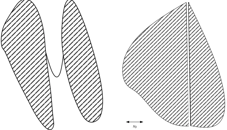
is an equivalence relation and its classes of equivalence are called connected components of C. At this point, in view of the formulation of the cluster assumption, it is very tempting to define the clusters as the connected components of C. However, this definition suffers from two major flaws:

1. a connected set cannot be defined up to a set of null Lebesgue measure. Indeed, consider for example the case d =1 and C= [0,1]. This set is obviously connected (take the map f equal to the identity on [0,1]) but the setCe=C_{\ {}1/2_} is not connected anymore even though C andC only differ by a set of null Lebesgue measure. In our setup we want toe impose connectedness on certain subsets of theλ-level set of the density p which is actually defined up to a set of null Lebesgue measure. Figure 1 (left) is an illustration of a set with one connected component whereas it is desirable to have two clusters.

2. There is no scale consideration in this definition of clusters. When two clusters are too close to each other in a certain sense, we wish identify them as a single cluster. In Figure 1 (right), the displayed set has two connected components whereas we wish to identify only one cluster.

To fix the first flaw, we introduce the following notions. Let

B

(z,r)be the d-dimensional closed ball of center z_∈IRd and radius r>0, defined by

B

(z,r) =nx_∈IRd:_kz₋x_{k ≤}r

o

,

wherek · kdenotes the Euclidean norm in IRd.

Definition 4.1 Fix r0≥0 and let d be an integer such that d≥d. We say that a measurable set C_⊂

X

is r0-standard if for any z∈C and any 0≤r≤r0, we have

Lebd

B

(z,r)∩C

≥c0rd. (5)

We now comment upon this definition.

Remark 4.1 The definition of a standard set has been introduced by Cuevas and Fraiman (1997). This definition ensures that the set C has no “flat” parts which allows to exclude pathological cases such as the one presented on the left hand side of Figure 1.

Remark 4.2 The constant c0may depend on r0 and this avoids large-scale shape considerations. Indeed, if the set C is bounded, then for any z_∈C, Lebd

B

(z,r)∩C

=Lebd C

for r_≥r0where r0 is the diameter of C. Thus for C to be r0-standard, we have to impose at least that c0≤Lebd C

r−₀d. Remark 4.3 The case d>d allows us to include a wide variety of shapes in this definition. Con-sider the following example where d=2:

Fix r≤√2 and consider the point z= (0,0). It holds

Lebd

B

(z,r)_∩C_δ≥

Z r0

−r0min(|x|

δ_,r0_{)dx, where r}0_=√r

2.

For any_|x_{| ≤}r0_≤1, we have_|x_|δ_{≥ |}x_|(δ∨1)and_|x_|(δ∨1)_{≤ |}r0_|(δ∨1)_≤r0. Thus

Lebd

B

(z,r)_∩C_δ≥

Z r0

−r0|x|

(δ∨1)_dx=2(r0₎(δ∨1)+1_.

We conclude that (5) is satisfied at z= (0,0)for d= (δ_∨1) +1. However, notice that

Lebd

B

(z,r)∩Cδ

≤

Z r

−r|

x_|δdx=2r(δ+1). Thus (5) is not satisfied at z= (0,0)when d=d, ifδ>1.

To overcome the scale problem described in the second flaw, we introduce the notion of s0 -separated sets.

Define the pseudo-distance distance d_∞, between two sets C1and C2by d∞(C1,C2) = inf

x∈C1

y∈C2

kx₋y_k.

We say that two sets C1,C2, are s0-separated if d∞(C1,C2)>s0, for some s0≥0. More generally, we say that the sets C1,C2, . . .are mutually s0-separated if for any j=6 j0, Cj and Cj0 are s₀-separated. On the right hand side of Figure 1, we show an example of two sets that are not s0-separated for a reasonable s0. In that particular example, if s0 is sufficiently small, we would like to identify a single cluster.

We now define s0-connectedness which is a weaker version of connectedness in the form of a binary relation

Definition 4.2 Fix s>0 and let_←→s

C be the binary relation defined on C⊂

X

as follows: two points x,y_∈C satisfy x_←→s

C y if and only if there exists a piecewise constant map f :[0,1]→C such that f(0) =x and f(1) =y and such that f has a finite number of jumps that satisfy_kf(t+)−f(t−)k ≤s

for any t∈[0,1], where

f(t+) =lim

θ→t θ>t

f(θ) and f(t₋) =lim θ→t θ<t

f(θ).

If x_←→s

C y, we say that x and y are s-connected.

Note that x and y are s-connected if and only if there exists z1, . . . ,zn∈C such thatkx−z1k ≤s,

Lemma 4.1 Fix s>0, then the binary relation←→s

C is an equivalence relation and C can be par-titioned into its classes of equivalence. The classes of equivalence of_←→s

C are called s-connected components of C.

In the next proposition we prove that given a certain scale s>0, it is possible split a r0-standard and closed set C into a unique partition that is a coarser than the partition defined by the connected components of C and that this partition is finite for such sets.

Proposition 4.1 Fix r0>0,s>0 and assume that C is a r0-standard and closed set. Then there exists a unique partition C1, . . .CJ, J≥1, of C such that

• for any j=1, . . . ,J and any x,y_∈Cj, we have x←→s C y,

• the sets C1, . . . ,CJ are mutually s-separated.

Remark 4.4 In what follows we assume that the scale s=s0 is fixed by the statistician. It should be fixed depending on a priori considerations about the scale of the problem. Actually, in the proof of Proposition 4.3, we could even assume that s0=1/(3 log m), which means that we can have the scale depend on the number of observations. This is consistent with the fact that the finite number of unlabeled observations allows us to have only a blurred vision of the clusters. In this case, we are not able to differentiate between two clusters that are too close to each other but our vision becomes clearer and clearer as m tends to infinity.

PSfrag replacements

r0

PSfrag replacements

s0

Figure 1: A set that is not r0-standard for any r0 (left). A set that has two connected components but only one s0-connected components (right).

Strong Cluster Assumption (SCA) Fix s0>0 and r0>0 and assume thatΓadmits a version that is r0-standard and closed. Denote by T1, . . . ,TJthe s0-connected components of this version of Γ. Then the function x_∈

X

_7→1I_{η(x)≥1/2_}takes a constant value on each of the Tj,j=1, . . .J. 4.2 Estimation of the Clusters

Assume that p is uniformly bounded by a constant L(p)and that

X

is bounded. Denote by IPmand IEmrespectively the probability and the expectation w.r.t the sampleXuof size m. Assume that we use the sampleXuto construct an estimator ˆGmofΓsatisfying

IEm

Lebd(Gˆm4Γ)

→0, m_→+∞,

where4is the sign for the symmetric difference. We call such estimators consistent estimators of Γ. Recall that we are interested in identifying the s0-connected components T1, . . . ,TJ ofΓ. That is, we seek a partition of ˆGm, denoted here by ˆH1, . . . ,_Hˆ_J0 such that for any j=1, . . . ,J, ˆH_j is a consistent estimator of Tj and IEm

Lebd(Hˆj)

→0 for j>J. From Proposition 4.1, we know that for any 1_≤ j,j0_≤J, j₆= j0, we have d_∞(Tj,Tj0)>s₀. Let s>s₀be defined by

s=min

j6=j0d∞(Tj,Tj0). (6)

To define the partition ˆH1, . . . ,HˆJ0, it is therefore natural to use a suitable reordering of the (s₀+ um)-connected components of ˆGm, where um is a positive sequence that tends to 0 as m tends to infinity. Since the measure of performance IEm

Lebd(Gˆm4Γ)

is defined up to a set of null Lebesgue measure it may be the case that even an estimator ˆGm that satisfies IEm

Lebd(Gˆm4Γ)

=0 has only one(s0+um)-connected components whereas Γhas several s0-connected components. This happens for example in the case where ˆGm=Γ∪R where R is a set of thin ribbons with null Lebesgue measure that link the s0-connected components ofΓto each other (see Figure 1, left). If

ˆ

Gmwere r0-standard, such configurations would not occur. To have ˆGmmore “standard”, we apply the following clipping transformation: define the set

Clip(Gˆm) =

x_∈Gˆm: Lebd Gˆm∩

B

(x,(log m)−1)

≤(log m)−

d

mα .

In the sequel, we will only consider the clipped version of ˆGmdefined by ˜Gm=Gˆm\Clip(Gˆm). For any x_∈G˜m, we have

Lebd Gˆm∩

B

(x,(log m)−1)

>(log m)− d

mα .

However, this is not enough to ensure that the union of several s0-connected components of Γis not estimated by a single(s0+um)-connected component of ˜Gmdue to the magnitude of random fluctuations of ˜GmaroundΓ.

To ensure componentwise consistency, we make assumptions on the estimator ˆGm. Note that the performance of a density level set estimator ˆGmis measured by the quantity

IEm

Lebd(Gˆm4Γ)

=IEm

Lebd(Gˆcm∩Γ)

+IEm

Lebd(Gˆm∩Γc)

. (7)

For some estimators, such as the offset plug-in density level sets estimators presented in Section 5, we can prove that the dominant term in the RHS of (7) is IEm

Lebd(Gˆcm∩Γ)

Definition 4.3 Let ˆGmbe an estimator ofΓand fixα>0. We say that the estimator ˆGmis consistent from inside at rate m−αif it satisfies

IEmLebd(Gˆm4Γ)

=Oe(m−α),

and

IEmLebd(Gˆm∩Γc)

=Oe(m−2α).

The following proposition ensures that the clipped version of an estimator that is consistent from inside is also consistent from inside at the same rate.

Proposition 4.2 Fixα>0,s0>0 and let(um)be a positive sequence. Assume that

X

is bounded and let ˆGm be an estimator of Γ that is consistent from inside at rate m−α. Then, the clipped estimator ˜Gm=Gˆm\Clip(Gˆm)is also consistent from inside a rate m−αand has a finite number

˜

Km≤Lebd(

X

)mα of (s0+um)-connected components that have Lebesgue measure greater than or equal to m−α. Moreover, the(s0+um)-connected components of ˜Gm are mutually(s0+θum) -separated for anyθ_∈(0,1).

We are now in position to define the estimators of the s0-connected components ofΓ. Define sm=

s0+ (3 log m)−1and denote by ˜H1, . . . ,H˜K˜m the sm-connected components of ˜Gmthat have Lebesgue

measure greater than or equal to m−α. The number ˜Kmdepends onXuand is therefore random but bounded from above by the deterministic quantity Lebd(

X

)mα.

Let

J

be a subset of_{1, . . . ,J_}. Defineκ(j) =_{k=1, . . . ,_K˜_{m: ˜Hk∩Tj6=}/0_{}and let D(}

J

_{)be the} event on which the setsκ(j),j_∈

J

are reduced to singletons_{k(j)_}that are disjoint, that is,

D(

J

) =nκ(j) =_{k(j)_},k(j)₆=k(j0),_∀j,j0_∈

J

,j₆=j0

o

=nκ(j) =_{k(j)_},(Tj∪H˜k(j))∩(Tj0∪H˜_k(j0₎) =/0, ∀j,j0∈

J

,j6= j0

o

.

(8)

In other words, on the event D(

J

), there is a one-to-one correspondence between the collection

{Tj}j∈J and the collection{H˜k}k∈κ(j) _j∈J. Componentwise convergence of ˜GmtoΓ, is ensured when D(_{1, . . . ,J_}) has asymptotically overwhelming probability. The following proposition en-sures that D(

J

)has large enough probability.

Proposition 4.3 Fix r0>0 and s0 _≥(3 log m)−1_{. Assume that there exists a version of Γthat is} r0-standard and closed. Then, denoting by J the number of s0-connected components ifΓ, for any

J

⊂ {1, . . . ,J}, we have

IPm Dc(

J

)) =O me −α

,

where

D

(

J

)is defined in (8).

4.3 Labeling the Clusters

THREE-STEP PROCEDURE

1. Use the unlabeled dataXuto construct an estimator ˆGmofΓthat is consistent from inside at rate m−α.

2. Define homogeneous regions as the sm-connected components of ˜Gm =Gˆm\ Clip(Gˆm)(clipping step) that have Lebesgue measure greater than or equal to m−α.

3. Assign a single label to each estimated homogeneous region by a majority vote on labeled data.

This method translates into two distinct error terms, one term in m and another term in n. We apply our three-step procedure to build a classifier ˜gn,mbased on the pooled sample(Xl,Xu). Fix α>0 and let ˆGmbe an estimator of the density level setΓ, that is consistent from inside at rate m−α. For any 1_≤k_≤K˜m, define the random variable

Z_nk_,m= n

∑

i=1

(2Yi−1)1I_{Xi∈H˜k},

where ˜Hk is obtained by Step 2 of the three-step procedure. Denote by ˜gkn,mthe function ˜gkn,m(x) = 1I_{Zk

n,m>0}for all x∈H˜kand consider the classifier defined on

X

by

˜

gn,m(x) = ˜ Km

∑

k=1 ˜

gk_n,m(x)1I_{x∈H˜_k}, x∈

X

. (9) Note that the classifier ˜gn,massigns label 0 to any x outside of ˜Gm. This is a notational convention and we can assign any value to x on this set since we are only interested in the cluster excess-risk. Nevertheless, it is more appropriate to assign a label referring to a rejection, for example, the values “2”or “R” (or any other value different from_{0,1_}). The rejection meaning that this point should be classified using labeled data only. However, when the amount of labeled data is too small, it might be more reasonable not to classify this point at all. This modification is of particular interest in the context of classification with a rejection option when the cost of rejection is smaller than the cost of misclassification (see, for example, Herbei and Wegkamp, 2006). Remark that when there is only a finite number of clusters, there existsδ>0 such that

δ= min j=1,...,J

_δ

j :δj>0 . (10)

Theorem 4.1 Fixα>0 and assume that (SCA) holds. Consider an estimator ˆGmofΓ, based on Xuthat is consistent from inside at rate m−α. Then, the classifier ˜gn,mdefined in (9) satisfies

E

Γ(g˜n,m)≤Oe

m−α 1₋θ

+ J

∑

j=1

δje−n(θδj)

2_/2 ≤Oe

m−α 1₋θ

+e−n(θδ)2/2, (11) for any 0<θ<1 and whereδ>0 is defined in (10).

5. Plug-in Rules for Density Level Sets Estimation

Fix λ>0 and recall that our goal is to use the unlabeled sample Xu of size m to construct an estimator ˆGmofΓ=Γ(λ) ={x∈

X

: p(x)≥λ}, that is consistent from inside at rate m−αfor some α>0 that should be as large as possible. A simple and intuitive way to achieve this goal is to use plug-in estimators ofΓdefined by

ˆ

Γ=Γˆ(λ) =_{x_∈

X

: ˆpm(x)≥λ},

where ˆpmis some estimator of p. A straightforward generalization are the offset plug-in estimators ofΓ(λ), defined by

˜

Γ`=Γ˜`(λ) ={x∈

X

: ˆpm(x)≥λ+`},

where` >0 is an offset. Clearly, we have ˜Γ`⊂Γˆ. Keeping in mind that we want estimators that are

consistent from inside we are going to consider sufficiently large offset`=`(m).

Plug-in rules is not the only choice for density level set estimation. Direct methods such as empirical excess mass maximization (see, for example, Polonik, 1995; Tsybakov, 1997; Steinwart et al., 2005) are also popular. One advantage of plug-in rules over direct methods is that once we have an estimator ˆpm, we can compute the whole collection{Γ˜`(λ),λ>0}, which might be of

interest for the user who wants to try several values ofλ. Note also that a wide range of density estimators is available in usual software. A density estimator can be parametric, typically based on a mixture model, or nonparametric such as histograms or kernel density estimators. In Section 6, we briefly describe a possible implementation based on existing software that makes use of kernel or nearest neighbors density estimators. To conclude this discussion, remark that the greater flexibility of plug-in rules may result in a poorer learning performance and even though we do not discuss any implementation based on direct methods, it may well be the case that the latter perform better in practice. However, it is not our intent to propose here the best clustering algorithm or the best density level set estimator and we present a simple proof of convergence for offset plug-in rules only for the sake of completeness.

The next assumption has been introduced in Polonik (1995). It is an analog of the margin assumption formulated in Mammen and Tsybakov (1999) and Tsybakov (2004) but for arbitrary levelλin place of 1/2.

Definition 5.1 For anyλ,γ_≥0, a function f :

X

_→IR is said to haveγ-exponent at levelλif there exists a constant c?>0 such that, for allε>0,

Lebd_{x_∈

X

:_|f(x)₋λ_{| ≤}ε_{} ≤}c?εγ.

Whenγ>0 it ensures that the function f has no flat part at levelλ.

The next theorem gives fast rates of convergence for offset plug-in rules when ˆpm satisfies an exponential inequality and p hasγ-exponent at levelλ. Moreover, it ensures that when the offset` is suitably chosen, the plug-in estimator is consistent from inside.

Theorem 5.1 Fixλ>0,γ>0 and ∆>0. Let ˆpm be an estimator of the density p based on the sample Xu of size m≥1 and let

P

be a class of densities on

X

. Assume that there exist positive constants c1,c2and a≤1, such that for PX-almost all x∈

X

, we have

sup p∈P

IPm(|pˆm(x)−p(x)| ≥δ)≤c1e−c2m

a_δ2

Assume further that p hasγ-exponent at levelλfor any p∈

P

and that the offset`is chosen as

`=`(m) =m−a2log m. (13)

Then the plug-in estimator ˜Γ`is consistent from inside at rate m− γa

2 for any p∈

P

.

Consider a kernel density estimator ˆpK_mbased on the sampleXudefined by

ˆ

pK_m(x) = 1

mhd n+m

∑

i=n+1 K

Xi−x h

, x_∈

X

,

where h>0 is the bandwidth parameter and K : IRd→IR is a kernel. If p is assumed to have H ¨older smoothness parameterβ>0 and if K and h are suitably chosen, it is a standard exercise to prove inequality of type (12) with a=2β/(2β+d). In that case, it can be shown that the rate m−γ2a is

optimal in a minimax sense (see Rigollet and Vert, 2006).

6. Discussion

We proposed a formulation of the cluster assumption in probabilistic terms. This formulation re-lies on Hartigan’s (1975) definition of clusters but it can be modified to match other definitions of clusters.

We also proved that there is no hope to improve the classification performance outside of these clusters. Based on these remarks, we defined the cluster excess-risk on which we observe the effect of unlabeled data. Finally we proved that when we have consistent estimators of the clusters, it is possible to achieve exponential rates of convergence for the cluster excess-risk. The theory developed here can be extended to any definition of clusters as long as they can be consistently estimated.

Note that our definition of clusters is parametrized by λwhich is left to the user, depending on his trust in the cluster assumption. Indeed, density level sets have the monotonicity property: λ≥λ0_{, impliesΓ(λ)⊂Γ(λ}0_{). In terms of the cluster assumption, it means that whenλdecreases}

to 0, the assumption (SCA) concerns bigger and bigger sets Γ(λ) and in that sense, it becomes more and more restrictive. As a result, the parameterλcan be considered as a level of confidence characterizing to which extent the cluster assumption is valid for the distribution P.

The choice ofλcan be made by fixing PX(

C

), where

C

is defined in (1), the probability of the rejection region. We refer to Cuevas et al. (2001) for more details. Note that data-driven choices ofλcould be easily derived if we impose a condition on the purity of the clusters, that is, if we are given theδin (10). Such a choice could be made by decreasingλuntil the level of purity is attained. However, any data-driven choice ofλhas to be made using the labeled data. It would therefore yield much worse bounds when nm.

instances that are affected to the same cluster as X . Observe that unlike the method described in the paper, the clusters depend on the labeled instances (X1, . . . ,Xn). Proceeding so allows us to use directly existing clustering algorithms without any modification. Since all three algorithms are distance based, we could run them only on unlabeled instance and then affect each labeled instance and the new instance to the same cluster as its nearest neighbor. However, if we assume that mn, incorporating labeled instances will not significantly affect the resulting clusters.

We now describe more precisely why these algorithms produce estimated clusters that are re-lated to the sm-connected components of a plug-in estimator of the density level set. Each algorithm has instances(X1, . . . ,Xm)and several parameters described below as inputs. Note that these clus-tering algorithms will affect every instance to a cluster. This can be transformed into our framework by removing clusters that contain only one instance.

• DBSCAN has two input parameters: a real numberε>0 and and integer M≥1. The basic version of this algorithm proceeds as follows. For a given instance Xi, let Jε(i)_{⊂ {}1, . . . ,m_} be the set of indexes j₆=i such that _kXj−Xik ≤ε. If card(Jε(i))≥M then all instances Xj,j∈Jε(i) are affected to the same cluster as Xi and the procedure is repeated with each Xj,j∈Jε(i). Otherwise a new cluster is defined and the procedure is repeated with another instance.

Observe first that the instances Xj that satisfy kXj−Xik ≤ε are ε-connected to Xi. Also, define the kernel density estimator ˆpmby:

ˆ pm(x) =

1 mεd

m

∑

j=1

K x−Xi

ε

,

where K : IRd_{→IR is defined by K(x) =1I}

{kxk≤1} for any x∈IRd. Then card(Jε(i))≥M is

equivalent to ˆpm(Xi)≥M_m+_εd1. Thus, if we chose s0=ε−(3 log m)−1andλ+`(m) =

M+1 mεd , we

see thatDBSCANimplements our method. Conversely, for givenλand s0, we can derive the parametersεand M such thatDBSCANimplements our method.

• OPTICS is a modification ofDBSCANthat allows the user to compute in an efficient fashion all cluster partitions for differentε_≤ε0for some user specifiedε0>0. The user still has to input the chosen value forεso that from our point of view, the two algorithms are the same.

• Both of the previous algorithms suffer from a major drawback that is inherent to our definition of cluster based on a global level when determining the density level sets. Indeed, in many real data sets, some clusters can only be identified using several density levels. Stuetzle (2003) recently described an algorithm called runt pruning that is free from this drawback. Since, it does not implement our method, we do not describe the algorithm in detail but mention it because it implements a more suitable definition of clusters that is also based on connectedness and density level sets. In particular it resolves the problem of choosingλ. It uses a nearest neighbor density estimator as a running horse and uses a single input parameter that corresponds to the scale s0.

among several available and it could be interesting to modify the formulation of the cluster assump-tion to match other definiassump-tions of cluster. In particular, the definiassump-tion of cluster as s0-connected components of theλ-level set of the density leaves the problem of choosingλcorrectly.

Acknowledgments

The author is most indebted to anonymous referees that contributed to a significant improvement of the paper through their questions and comments.

Appendix A. Proofs

This section contains proofs of the results presented in the paper.

A.1 Proof of Proposition 2.1

Since the distribution of the unlabeled sampleXudoes not depend onη, we have for any marginal distribution PX,

sup η∈Ξ

IEn,m

Z

Cc|2η−1|1I{Tn,m6=g

?_}dP_X =sup

η∈Ξ

IEmIEn

hZ

Cc|2η−1|1I{Tn,m6=g

?_}dPX

_Xui

=IEmsup η∈Ξ

IEn

hZ

Cc|2η−1|1I{Tn,m6=g

?_}dP_XX_u

i

≥inf Tn

sup η∈Ξ

IEn

Z

Cc|2η−1|1I{Tn6=g

?_}dP_X,

where in the last inequality, we used the fact that conditionally onXu, the classifier Tn,monly depends onXl and can therefore be written Tn.

A.2 Proof of Theorem 3.1

We can decompose

E

_C(gˆn)into

E

C(gˆn) =IEn

∑

j≥1

Z

Tj

|2η(x)₋1_|1I_{gˆj

n(x)6=g?(x)}p(x)dx.

Fix j_{∈ {}1,2, . . ._}and assume w.l.o.g. thatη_≥1/2 on Tj. It yields g?(x) =1,∀x∈Tj, and since ˆgn is also constant on Tj, we get

Z

Tj

|2η(x)₋1_|1I

{gˆnj(x)6=g?(x)}p(x)dx=1I{Znj≤0}

Z

Tj

(2η(x)₋1)p(x)dx

≤δj1I

|δj−Z j n n|≥δj

. (14)

Taking expectation IEnon both sides of (14) we get

IEn

Z

Tj

|2η(x)₋1_|1I

{gˆnj(x)6=g?(x)}p(x)dx≤δjIPn h_δ

j− Znj

n

_≥δj

i

≤2δje−nδ

where we used Hoeffding’s inequality to get the last bound. Summing now over j yields the theo-rem.

A.3 Proof of Lemma 4.1

The binary relation_←→s

C is an equivalence relation if it satisfies reflexivity, symmetry and transitivity. To prove reflexivity, consider the trivial constant path f(t) =x for all t_∈[0,1]. We immediately obtain that x_←→s

C x.

To prove symmetry, fix x,y_∈C such that x_←→s

C y and denote by f1the piecewise constant map with n1jumps that satisfies f1(0) =x, f1(1) =y andkf1(t+)−f1(t−)k ≤s. It is not difficult to see

that the map ˜f1 defined by ˜f1(t) = f1(1−t)for any t∈[0,1]is piecewise constant with n1jumps, satisfies ˜f1(0) =y, ˜f1(1) =x andkf˜1(t+)−f˜1(t−)k ≤s for any t∈[0,1], so that y←→s

C x. To prove transitivity, let z_∈C be such that y_←→s

C z and let f2be a piecewise constant map with n2 jumps that satisfies f2(0) =y, f2(1) =z and kf2(t+)−f2(t−)k<s for any t∈[0,1]. Let now

f :[0,1]_→

X

be the map defined by:

f(t) =

f1(2t) if t∈[0,1/2] f2(2t−1) if t∈[1/2,1].

This map is obviously piecewise constant with n1+n2jumps and satisfies f(0) =x,f(1) =z. More-over, for any t_∈[0,1], f satisfies_kf˜(t+)−f˜(t−)k ≤s.

Thus_←→s

C is an equivalence relation and C can be partitioned into its classes of equivalence.

A.4 Proof of Proposition 4.1

From Lemma 4.1, we know that _←→s

C is an equivalence relation and C can be partitioned into its classes of equivalence denoted by C1,C2, . . .. The classes of equivalences C1,C2, . . .obviously sat-isfy the first point of Proposition 4.1 from the very definition of a class of equivalence.

To check the second point, remark first that since C is a closed set, each Cj,j_≥1 is also a closed set. Indeed, fix some j_≥1 and let(xn,n≥1)be a sequence of points in Cjthat converges to x. Since C is closed, we have x∈C so there exists j0≥1 such that x∈Cj0. If j=6 j0, thenkx_n−xk>s for any n_≥1 which contradicts the fact that xnconverges to x. Therefore, x_∈Cjand Cjis closed. Then let Cj and Cj0, be two classes of equivalence such that d_∞(C_j,C_j0)≤s. Using the fact that C_j and Cj0 are closed sets, we conclude that there exist x∈C_jand x0∈C_j0 such thatkx−x0k ≤s and hence that x_←→s

C x

0_{. Thus Cj=Cj0 and we conclude that for any Cj,Cj0,j6= j}0_{, we have d∞(Cj,Cj0)>s}

and the Cj are mutually s-separated.

We now prove that the decomposition is finite. Since the Cj are mutually s-separated, for any 1_≤ j_≤k, for any xj∈Cj, the Euclidean balls

B

(xj,s/3)are disjoint. Using the facts that

X

is bounded and that C is r0-standard we obtain,

∞>Lebd(

X

)≥ k

∑

j=1 Lebd

B

(xj,s/3)∩

X

≥

k

∑

j=1 Lebd

B

(xj,s/3)∩C

for a positive constant c. Thus we proved the existence of a finite partition

C= J

[

j=1 Cj.

It remains to prove that this partition is unique. To this end, we make use of the fundamental theorem of equivalence relations (see, for example, Dummit and Foote, 1991, Prop. 2, page 3) which states that any partition of C corresponds to the classes of equivalences of a unique equivalence relation. Let

P

0=_{C₁0, . . . ,C_J00}be a partition of C that satisfies the two points of Proposition 4.1 and denote by

R

0 the corresponding equivalence relation. We now prove that _←→s

C ≡

R

0_{. From}

the first point of Proposition 4.1, we easily conclude that if x

R

0y then x_←→s

C y. Now if we choose x,y_∈C such that x

R

0y does not hold, then there exist j₆= j0 such that x_∈C0_j and y_∈C0_j0. If we

had x_←→s

C y, it would hold d∞(C

0

j,C0j0)≤s which contradicts the second point of Proposition 4.1 so

x_←→s

C y does not hold. As a consequence we have proved that for any x,y∈C, x

R

y if and only if x_←→s

C y and the two relations are the same so as their classes of equivalence. This allows us to conclude that

P

0=

P

.

A.5 Proof of Proposition 4.2

Consider a regular grid

G

on IRd _{with step size 1/log(m) and observe that the Euclidean balls of} centers in ˜

G

=

G

_∩Clip(Gˆm)and radius

√

d/log(m)cover the set Clip(Gˆm). Since

X

is bounded, there exists a constant c1>0 such that card{

G

˜}=c1(log m)d. Therefore

Lebd(Clip(_Gˆ_m))≤

∑

x∈_G˜

Lebd

B

(x,√d/log(m))_∩Gˆ_m≤c2(log m)d−d

mα ,

for some positive constant c2. Therefore, the rate of convergence ˜Gm is the same as that of ˆGm. Observe also that ˜Gm⊂Gˆm, so that ˜Gmis also consistent from inside.

Assume that ˜Gmcan be decomposed in at least a number k of(s0+um)-connected components, ˜

H1, . . . ,H˜k with Lebesgue measure greater than or equal to m−α. It holds

∞>Lebd(

X

)_≥ k

∑

j=1

Lebd(_T˜_j)≥km−α_,

Therefore, the number of(s0+um)-connected components of ˜Gm with Lebesgue measure greater than or equal to m−αis at most Lebd(

X

)mα.

A.6 Proof of Proposition 4.3

Define m0=e 1

3(r0∧s0) _{and denote D(}

J

_{)by D. Remark that}

Dc= J

[

j=1

A1(j)∪A2(j)∪A3(j),

where

A1(j) ={card[κ(j)] =0}, A2(j) ={card[κ(j)]≥2}, A3(j) =

[

j0_6=j

{κ(j)_∩κ(j0)₆=/0_}.

In words, A1(j) is the event on which Tj is estimated by none of the(_H˜_{k)k, A2(j) is the event on} which Tjis estimated by at least two different elements of the collection(H˜k)kand A3(j)is the event on which Tj is estimated by an element of the collection(H˜k)k that also estimates another Tj0 from the collection(Tj)j.

For any j=1, . . . ,J, we have

A1(j) ={card[κ(j)] =0} ⊂ {Tj⊂G˜m4Γ} ⊂ {

B

(x,r)∩Tj⊂G˜m4Γ},

for any x_∈Tj and r>0. Remark that from Proposition 4.1, the Tj are mutually s0-separated so we have

B

(x,r)_∩Tj=

B

(x,r)∩Γfor any r≤s0. Thus, for any m≥m0, it holds(3 log m)−1≤s0∧r0 and

A1(j)⊂ {Lebd[

B

(x,(3 log m)−1)∩Tj]≤Lebd[G˜m4Γ]} ⊂ {Lebd[G˜m4Γ]≥c0(3 log m)−d}, where in the last inclusion we used the fact thatΓis r0-standard.

We now treat A2(j). Assume without loss of generality that{1,2} ⊂κ(j). On A2(j), there exist x1∈Tj∩H˜1, xn∈Tj∩H˜2and a sequence x2, . . . ,xn−1∈Tjsuch thatkxj−xj+1k ≤s0. Observe now that from Proposition 4.2, we have_kx1−xnk>s0≥(3 log m)−1for m≥m0. Therefore the integer

j?=minj : 2_≤ j_≤n,_∃z_∈H˜1s.t.kxj−zk>(3 log m)−1 ,

is well defined. Moreover, there exists z0∈H˜1 such thatkxj?₋₁−z₀k ≤(3 log m)−1. Now, if there

exists z∈_H˜_{k, for some k∈ {2, . . . ,K}˜_{m}, such thatkxj}?−zk ≤(3 log m)−1, then

d∞(_H˜_1,H˜_{k)≤ kz0−xj}?₋₁k+kx_j?₋₁−x_j?k+kx_j?−zk ≤s₀+2(3 log m)−1.

This contradicts the conclusion of Proposition 4.2 which states that d_∞(_H˜_1,H˜_{k)>s0+θ(log m)}−1 for any k=2, . . . ,_K˜_{m in particular whenθ=2/3. Therefore we obtain that on A2(j)there exists} xj?∈T_j such that

B

(xj?,(3 log m)−1)∩G˜_m= /0.

It yields

A2(j)⊂

B

(xj?,(3 log m)−1)∩T_j⊂G˜_m4Γ

⊂LebdG˜m4Γ

where in the second inclusion used the fact that

B

(xj?,r)∩T_j=

B

(x_j?,r)∩Γfor any r≤s₀and that

Γis r0-standard.

We now consider the event A3(j). Assume without loss of generality that j=1 and let k be such that k∈κ(1)_∩κ(j0)for some j0∈ {2, . . . ,J}. On A3(1), there exist y1∈T1∩H˜k, yn∈Tj0∩H˜_kand a sequence y2, . . . ,yn₋1∈H˜ksuch thatkyj−yj+1k ≤sm.

Observe now that from Proposition 4.1, we have _ky1−ynk>s0≥(3 log m)−1 for m≥m0. Therefore the integer

j]=minj : 2≤ j≤n,_∃z∈T1s.t.kyj−zk>(3 log m)−1 ,

is well defined. Moreover, there exists z1∈T1such thatkyj]₋₁−z₁k ≤(3 log m)−1. Now, if there

exists z_∈Tj0 for some j0∈ {2, . . . ,J}such thatky_j]−zk ≤(3 log m)−1, then

d∞(T1,Tj0)≤ ky_j]₋₁−z1k+kyj]₋₁−y_j]k+ (3 log m)−1≤s0+ (log m)−1<s,

for sufficiently large m and where s is defined in (6). This contradicts the definition of s which implies that d_∞(T1,Tj0)≥s for any j∈ {2, . . . ,J}. Therefore we obtain that on A₃(1)there exists y_j]∈H˜_k such that

B

(y_j],(3 log m)−1)⊂Γc. It yields

A3(1)⊂

Lebd(G˜m∩Γc)≥Lebd(G˜m∩

B

(yj],(3 log m)−1)) .

Since y_j] ∈G˜m⊂Gˆm, we have Lebd(Gˆm∩

B

(yj],(3 log m)−1))≥m−α(3 log m)−d. On the other

hand, we have

Lebd(_G˜_m∩

_B

_(yj],(3 log m)−1)) =Lebd(Gˆ_m∩

B

(y_j],(3 log m)−1))

−Lebd(Clip(Gˆm)∩

B

(yj],(3 log m)−1))

≥m−α(3 log m)−d₋Lebd(Gˆm∩Γc)

≥m−α(3 log m)−d₋c3m−1.1α

≥c4m−α(log m)−d,

where we used the fact that ˆGmis consistent from inside at rate m−α. Hence,

A3(j) =

[

j0_6=j

{κ(j)_∩κ(j0)₆=/0_{} ⊂}Lebd(G˜m∩Γc)≥c5m−α(log m)−d .

Combining the results for A1(j), A2(j)and A3(j), we have IPm(Dc)≤IPm

Lebd

_˜

Gm4Γ

>c0(3 log m)−d +IPm

Lebd(G˜m∩Γc)≥c5m−α(log m)−d . Using the Markov inequality for both terms we obtain

IPm

Lebd

_˜

Gm4Γ

>c0(3 log m)−d =O me −α

,

and

IPm

Lebd(G˜m∩Γc)≥c5m−α(log m)−d =O me −α

,

A.7 Proof of Theorem 4.1

The cluster excess-risk

E

_Γ(g˜n,m)can be decomposed w.r.t the event D and its complement. It yields

E

Γ(g˜n,m)≤IEm

1IDIEn

Z

Γ|2η(x)−1|1I{g˜n,m(x)6=g?(x)}p(x)dx Xu

+IPm(Dc).

We now treat the first term of the RHS of the above inequality, that is, on the event D. Fix j_∈

{1, . . . ,J_}and assume w.l.o.g. that η_≥1/2 on Tj. Simply write Zk for Zkm,n. By definition of D, there is a one-to-one correspondence between the collection_{Tj}j and the collection{H˜k}k. We denote by ˜Hj the unique element of{H˜k}k such that ˜Hj∩Tj 6= /0. On D, for any j=1, . . . ,J, we have,

IEn

Z

Tj

|2η(x)₋1_|1I_{g˜j

n,m(x)6=g?(x)}p(x)dx Xu ≤ Z

Tj\G˜m

(2η₋1)dPX+IEn

1I_{Zj_≤0}

Z

Tj∩H˜j

(2η₋1)dPX

Xu

≤L(p)Lebd(Tj\G˜m) +δjIPn Zj≤0|Xu).

On the event D, for any 0<θ<1, it holds

IPn Zj≤0|Xu) =IPn

Z

Tj

(2η₋1)dPX−Zj≥δj|Xu

≤IPn

Zj₋

Z

˜ Hj

(2η₋1)dPX

_≥θδj|Xu

+1In PX

Tj4H˜j

≥(1−θ)δj

o_.

Using Hoeffding’s inequality to control the first term, we get

IPn Zj≤0|Xu)≤2e−n(θδj)

2_/2

+1In PX

Tj4H˜j

≥(1−θ)δj

o_.

Taking expectations, and summing over j, the cluster excess-risk is upper bounded by

E

Γ(g˜n,m)≤ 2L(p)

1₋θIEm

h

Lebd(Γ4G˜m)

i

+2 J

∑

j=1

δje−n(θδj)

2_/2

+IPm(Dc),

where we used the fact that on D,

J

∑

j=1 Lebd

Tj4H˜j

≤Lebd

_Γ

4G˜m

.

From Proposition 4.3, we have IPm(Dc) =Oe(m−α) and IEm

h

Lebd(Γ4G˜m)

i