Plug-and-Play Dual-Tree Algorithm Runtime Analysis
Ryan R. Curtin [email protected]
School of Computational Science and Engineering Georgia Institute of Technology
Atlanta, GA 30332-0250, USA
Dongryeol Lee [email protected]
Yahoo Labs
Sunnyvale, CA 94089
William B. March [email protected]
Institute for Computational Engineering and Sciences University of Texas, Austin
Austin, TX 78712-1229
Parikshit Ram [email protected]
Skytree, Inc. Atlanta, GA 30332
Editor:Nando de Freitas
Abstract
Numerous machine learning algorithms contain pairwise statistical problems at their core— that is, tasks that require computations over all pairs of input points if implemented naively. Often, tree structures are used to solve these problems efficiently. Dual-tree algorithms can efficiently solve or approximate many of these problems. Using cover trees, rigorous worst-case runtime guarantees have been proven for some of these algorithms. In this paper, we present aproblem-independent runtime guarantee foranydual-tree algorithm using the cover tree, separating out the problem-dependent and the problem-independent elements. This allows us to just plug in bounds for the problem-dependent elements to get runtime guarantees for dual-tree algorithms for any pairwise statistical problem without re-deriving the entire proof. We demonstrate this plug-and-play procedure for nearest-neighbor search and approximate kernel density estimation to get improved runtime guarantees. Under mild assumptions, we also present the first linear runtime guarantee for dual-tree based range search.
Keywords: dual-tree algorithms, adaptive runtime analysis, cover tree, expansion con-stant, nearest neighbor search, kernel density estimation, range search
1. Dual-tree Algorithms
prohibitive O(N2) time. Kernel density estimation is also a pairwise statistical problem, since we compute a sum over all reference points for each query point. This again requires
O(N2) time to answer O(N) queries if done directly. The reference set is typically indexed with spatial data structures to accelerate this type of computation (Finkel and Bentley, 1974; Beygelzimer et al., 2006); these result inO(logN) runtime per query under favorable conditions.
Building upon this intuition, Gray and Moore (2001) generalized the fast multipole method from computational physics to obtain dual-tree algorithms. These are extremely useful when there are large query sets, not just a few query points. Instead of building a tree on the reference set and searching with each query point separately, Gray and Moore suggest also building a query tree and traversing both the query and reference trees simultaneously (adual-tree traversal, from which the class of algorithms takes its name).
Dual-tree algorithms can be easily understood through the recent framework of Curtin et al. (2013b): two trees (a query tree and a reference tree) are traversed by apruning dual-tree traversal. This traversal visits combinations of nodes from the trees in some sequence (each combination consisting of a query node and a reference node), calling a problem-specific Score() function to determine if the node combination can be pruned. If not, then a problem-specific BaseCase() function is called for each combination of points held in the query node and reference node. This has significant similarity to the more common single-tree branch-and-bound algorithms, except that the algorithm must recurse into child nodes of boththe query tree and reference tree.
There exist numerous dual-tree algorithms for problems as diverse as kernel density estimation (Gray and Moore, 2003), mean shift (Wang et al., 2007), minimum spanning tree calculation (March et al., 2010),n-point correlation function estimation (March et al., 2012), max-kernel search (Curtin et al., 2013c), particle smoothing (Klaas et al., 2006), variational inference (Amizadeh et al., 2012), range search (Gray and Moore, 2001), and embedding techniques (Van Der Maaten, 2014), to name a few.
Some of these algorithms are derived using the cover tree (Beygelzimer et al., 2006), a data structure with compelling theoretical qualities. When cover trees are used, dual-tree all-nearest-neighbor search and approximate kernel density estimation have O(N) runtime guarantees forO(N) queries (Ram et al., 2009a); minimum spanning tree calculation scales as O(NlogN) (March et al., 2010). Other problems have similar worst-case guarantees (Curtin and Ram, 2014; March, 2013).
In this work we combine the generalization of Curtin et al. (2013b) with the theoretical results of Beygelzimer et al. (2006) and others in order to develop a worst-case runtime bound for any dual-tree algorithm when the cover tree is used.
Symbol Description
N A tree node
Ci Set of child nodes ofNi
Pi Set of points held inNi
Dn
i Set of descendant nodes ofNi
Dp
i Set of points contained inNi andDin
µi Center ofNi
λi Furthest descendant distance fromµi
Table 1: Notation for trees. See Curtin et al. (2013b) for details.
bounds for each of those algorithms. Each of these bounds is an improvement on the state-of-the-art, and in the case of range search, is the first such bound. Despite the intuition this provides for the scaling properties of all dual-tree algorithms1, it must be kept in mind that these worst-case bounds only apply to dual-tree algorithms that use the cover tree and the standard cover tree traversal.
2. Preliminaries
For simplicity, the algorithms considered in this paper will be presented in a tree-independent context, as in Curtin et al. (2013b), but the only type of tree we will consider is the cover tree (Beygelzimer et al., 2006), and the only type of traversal we will consider is the cover tree pruning dual-tree traversal, which we will describe later.
As we will be making heavy use of trees, we must establish notation (taken from Curtin et al., 2013b). The notation we will be using is defined in Table 1.
2.1 The Cover Tree
The cover tree is a leveled hierarchical data structure originally proposed for the task of nearest neighbor search by Beygelzimer et al. (2006). Each node Ni in the cover tree is
associated with a single point pi. An adequate description is given in their work (we have adapted notation slightly):
Acover tree T on a datasetS is a leveled tree where each level is a “cover” for the level beneath it. Each level is indexed by an integer scalesi which decreases
as the tree is descended. Everynodein the tree is associated with a point in S. EachpointinS may be associated with multiple nodes in the tree; however, we require that any point appears at most once in every level. Let Csi denote the
set of points in S associated with the nodes at level si. The cover tree obeys the following invariants for allsi:
• (Nesting). Csi ⊂Csi−1. This implies that once a point p ∈ S appears in
Csi then every lower level in the tree has a node associated withp.
• (Covering tree). For every pi ∈ Csi−1, there exists a pj ∈ Csi such that
d(pi, pj)<2si and the node in levelsi associated withpj is a parent of the
node in level si−1 associated withpi.
• (Separation). For all distinctpi, pj ∈Csi,d(pi, pj)>2
si.
As a consequence of this definition, if there exists a node Ni, containing the point pi
at some scalesi, then there will also exist a self-child node Nic containing the pointpi at
scale si−1 which is a child of Ni. In addition, every descendant point of the node Ni is
contained within a ball of radius 2si+1 centered at the point pi; therefore, λi = 2si+1 and
µi=pi (Table 1).
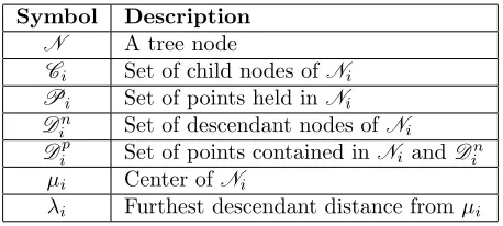
Note that the cover tree may be interpreted as an infinite-leveled tree, with C∞ con-taining only the root point,C−∞=S, and all levels between defined as above. Beygelzimer et al. (2006) find this representation (which they call the implicitrepresentation) easier for description of their algorithms and some of their proofs. But clearly, this is not suitable for implementation; hence, there is anexplicitrepresentation in which all nodes that have only a self-child are coalesced upwards (that is, the node’s self-child is removed, and the children of that self-child are taken to be the children of the node). Figure 1 shows each of the levels of an example cover tree (in the explicit representation) on a simple six-point dataset.
In this work, we consider only the explicit representation of a cover tree, and do not concern ourselves with the details of tree construction2.
2.2 Expansion Constant
The explicit representation of a cover tree has a number of useful theoretical properties based on the expansion constant (Karger and Ruhl, 2002); we restate its definition below.
Definition 1 Let BS(p,∆) be the set of points inS within a closed ball of radius∆around some p ∈ S with respect to a metric d: BS(p,∆) = {r ∈ S: d(p, r) ≤ ∆}. Then, the expansion constant of S with respect to the metric dis the smallest c≥2 such that
|BS(p,2∆)| ≤c|BS(p,∆)| ∀ p∈S, ∀ ∆>0. (1)
The expansion constant is used heavily in the cover tree literature. It is, in some sense, a notion of instrinic dimensionality, most useful in scenarios where c is independent of the number of points in the dataset (Karger and Ruhl, 2002; Beygelzimer et al., 2006; Krauthgamer and Lee, 2004; Ram et al., 2009a). Note also that if points in S ⊂ H are being drawn according to a stationary distributionf(x), thencwill converge to some finite value cf as |S| → ∞. To see this, define cf as a generalization of the expansion constant
for distributions. cf ≥2 is the smallest value such that
Z
BH(p,2∆)
f(x)dx≤cf
Z
BH(p,∆)
f(x)dx (2)
p0 p1 p2
p3 p4 p5
4
Na
(a) Root node at scale 1.
p0
p1 p2
p3 p4 p5
2
2
Nb
Nc
(b) Nodes at scale 0.
p0
p1 p2
p3 p4 p5
1 1
Nd
Ne
(c) Nodes at scale−1.
N2 N5 N1 N3
Na
Nb Nc
Nd Ne
N0 N4
scale 1
scale 0
scale−1
scale−∞
(d) Abstract representation.
Figure 1: Example cover tree on six points inR2. (a)N
ais centered atp0with scale 1. (b)
Nb and Ncare centered at p0 and p1, respectively, and have scale 0. (c)Nd and
Ne are centered at p0 and p2, respectively, and have scale −1. The leaves, N0
throughN6, are centered at each of the six points, with scale−∞(and therefore
radius 0). Note that although nodeNb in subfigure (b) overlaps nodeNc, point p1 only belongs to Nc, not Nb. Note also that this is only one valid cover tree
for all p∈ H and ∆>0 such thatR
BH(p,∆)f(x)dx > 0, and with BH(p,∆) defined as the
closed ball of radius ∆ in the spaceH.
As a simple example, takef(x) as a uniform spherical distribution inRd: for any|x| ≤1, f(x) is a constant; for|x|>1,f(x) = 0. It is easy to see thatcf in this situation is 2d, and
thus for some dataset S,c must converge to that value as more and more points are added to S. Closed-form solutions for cf for more complex distributions are less easy to derive;
however, empirical speedup results from Beygelzimer et al. (2006) suggest the existence of datasets where c is not strongly dependent on d. For instance, the covtype dataset has 54 dimensions but the expansion constant is much smaller than other, lower-dimensional datasets.
There are some other important observations about the behavior of c. Adding a single point to S may increase c arbitrarily: consider a set S distributed entirely on the surface of a unit hypersphere. If one adds a single point at the origin, producing the set S0, then
c explodes to |S0| whereas before it may have been much smaller than |S|. Adding a single point may also decrease c significantly. Suppose one adds a point arbitrarily close to the origin to S0; now, the expansion constant will be |S0|/2. Both of these situations are degenerate cases not commonly encountered in real-world behavior; we discuss them in order to point out that although we can bound the behavior ofc as|S| → ∞forS from a stationary distribution, we are not able to easily say much about its convergence behavior. The expansion constant can be used to show a few useful bounds on various properties of the cover tree; we restate these results below, given some cover tree built on a datasetS
with expansion constantc and |S|=N:
• Width bound: no cover tree node has more than c4 children (Lemma 4.1, Beygelz-imer et al., 2006).
• Depth bound: the maximum depth of any node isO(c2logN) (Lemma 4.3, Beygelz-imer et al., 2006).
• Space bound: a cover tree has O(N) nodes (Theorem 1, Beygelzimer et al., 2006).
Lastly, we introduce a convenience lemma of our own which is a generalization of the packing arguments used by Beygelzimer et al. (2006). This is a more flexible version of their argument.
Lemma 1 Consider a dataset S with expansion constant c and a subset C ⊆S such that every two distinct points inC are separated by at least δ. Then, for any pointp(which may or may not be in S), and any radiusρδ >0:
|BS(p, ρδ)∩C| ≤c2+dlog2ρe. (3)
Proof The proof is based on the packing argument from Lemma 4.1 in Beygelzimer et al. (2006). Consider two cases: first, letd(p, pi)> ρδfor anypi∈S. In this case,BS(p, ρδ) =∅
definition of the expansion constant. Because each point inCis separated byδ, the number of points inBS(p, ρδ)∩C is bounded by the number of disjoint balls of radiusδ/2 that can be packed into BS(p, ρδ). In the worst case, this packing is perfect, and
|BS(p, ρδ)| ≤ |BS(pi,2ρδ)| |BS(pi, δ/2)|
≤c2+dlog2ρe. (4)
3. Tree Imbalance
It is well-known that imbalance in trees leads to degradation in performance; for instance, a kd-tree node with every descendant in its left child except one is effectively useless. A
kd-tree full of nodes like this will perform abysmally for nearest neighbor search, and it is not hard to generate a pathological dataset that will cause akd-tree of this sort.
This sort of imbalance applies to all types of trees, not justkd-trees. In our situation, we are interested in a better understanding of this imbalance for cover trees, and thus endeavor to introduce a more formal measure of imbalance which is correlated with tree performance. Numerous measures of tree imbalance have already been established; one example is that proposed by Colless (1982), and another is Sackin’s index (Sackin, 1972), but we aim to capture a different measure of imbalance that uses the leveled structure of the cover tree.
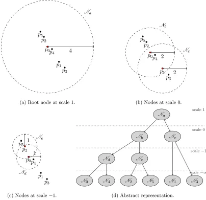
We already know each node in a cover tree is indexed with an integer level (or scale). In the explicit representation of the cover tree, each non-leaf node has children at a lower level. But these children need not be strictly one level lower; see Figure 2. In Figure 2a, each cover tree node has children that are strictly one level lower; we will refer to this as a perfectly balanced cover tree. Figure 2b, on the other hand, contains the nodeNm which
has two children with scale two less than sm. We will refer to this as an imbalanced cover tree. Note that in our definition, the balance of a cover tree has nothing to do with differing number of descendants in each child branch but instead only missing levels.
An imbalanced cover tree can happen in practice, and in the worst cases, the imbalance may be far worse than the simple graphs of Figure 2. Consider a dataset with a single
Nh Ni Nj
Nd
Nc
Nb
Nk
Na
Ng
Nf
Ne
sa
sa−1
sa−2
(a) Balanced cover tree.
Nr Ns
Nn
Nt
Nm
Nq
Np
sm
sm−1
sm−2
(b) Imbalanced cover tree.
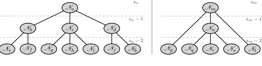
outlier
Figure 3: Single-outlier cover tree.
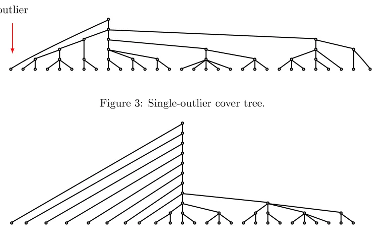
Figure 4: A multiple-outlier cover tree.
outlier which is very far away from all of the other points3. Figure 3 shows what happens in this situation: the root node has two children; one of these children has only the outlier as a descendant, and the other child has the rest of the points in the dataset as a descendant. In fact, it is easy to find datasets with a handful of outliers that give rise to a chain-like structure at the top of the tree: see Figure 4 for an illustration4.
A tree that has this chain-like structure all the way down, which is similar to thekd-tree example at the beginning of this section, is going to perform horrendously; motivated by this observation, we define a measure of tree imbalance.
Definition 2 The cover node imbalance In(Ni) for a cover tree node Ni with scale si in the cover tree T is defined as the cumulative number of missing levels between the node and its parent Np (which has scale sp). If the node is a leaf (that is, si =−∞), then the number of missing levels is defined as the difference between sp and smin−1 where smin is the smallest scale of a non-leaf node in T. IfNi is the root of the tree, then the cover node imbalance is 0. Explicitly written, this calculation is
In(Ni) =
sp−si−1 if Ni is not a leaf and not the root node
max(sp−smin−1, 0) if Ni is a leaf
0 if Ni is the root node.
(5)
3. Note also that for an outlier sufficiently far away, the expansion constant isN−1, so we should expect poor performance with the cover tree anyway.
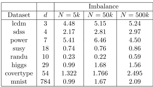
Imbalance
Dataset d N = 5k N = 50k N = 500k
lcdm 3 4.48 5.15 5.24
sdss 4 2.17 2.81 2.97
power 7 5.41 6.46 4.50
susy 18 0.74 0.76 0.86
randu 10 0.23 0.22 0.59
higgs 29 0.99 1.68 1.56
covertype 54 1.322 1.766 2.495
mnist 784 0.99 1.67 2.09
Table 2: Empirically calculated tree imbalances, normalized byN.
This simple definition of cover node imbalance is easy to calculate, and using it, we can generalize to a measure of imbalance for the full tree.
Definition 3 The cover tree imbalance It(T) for a cover tree T is defined as the cumula-tive number of missing levels in the tree. This can be expressed as a function of cover node imbalances easily:
It(T) = X
Ni∈T
In(Ni). (6)
A perfectly balanced cover tree Tb with no missing levels has imbalanceIt(Tb) = 0 (for
instance, Figure 2a). A worst-case cover treeTw which is entirely a chain-like structure with
maximum scalesmaxand minimum scalesmin will have imbalanceIt(Tw)∼N(smax−smin).
Because of this chain-like structure, each level has only one node and thus there are at least
N levels; or, smax−smin ≥N, meaning that in the worst case the imbalance is quadratic inN.5
However, for most real-world datasets with the cover tree implementation in mlpack
(Curtin et al., 2013a) and the reference implementation (Beygelzimer et al., 2006), the tree imbalance is near-linear with the number of points. We have constructed cover trees onN
uniformly subsampled points from a variety of datasets and calculated the imbalance; see Table 2 for the results. Ten trials were performed for each dataset and each N, and the mean imbalance is given. These results are normalized with respect to N, for which the values of 5000, 50000, and 500000 were chosen. The ‘power’, ‘susy’, ‘higgs’, and ‘covertype’ datasets are found in the UCI Machine Learning Repository (Bache and Lichman, 2013), the ‘mnist’ dataset is from LeCun et al. (2000), the ‘lcdm‘ and ‘sdss’ datasets are Sloan Digital Sky Survey data (Adelman-McCarthy et al., 2008), and the ‘randu’ dataset is randomly-generated uniformly-distributed data in 10 dimensions. The imbalances on each of these datasets tend to be near-linear.
Currently, no cover tree construction algorithm specifically aims to minimize imbalance.
Algorithm 1 The standard pruning dual-tree traversal for cover trees.
1: Input: query nodeNq, set of reference nodes R 2: Output: none
3: smaxr ←maxNr∈Rsr 4: if (sq< smaxr ) then
5: {Perform a reference recursion.} 6: for each Nr∈R do
7: BaseCase(pq, pr) 8: end for
9: Rr← {Nr∈R:sr=smaxr }
10: Rr−1← {C(Nr) :Nr∈Rr} ∪(R\Rr) 11: R0r−1← {Nr∈Rr−1 :Score(Nq,Nr)6=∞} 12: recurse with Nq and Rr−10
13: else
14: {Perform a query recursion.} 15: for each Nqc∈C(Nq)do
16: R0 ← {Nr∈R:Score(Nqc,Nr)6=∞} 17: recurse withNqc and R0
18: end for
19: end if
4. General Runtime Bound
Perhaps more interesting than measures of tree imbalance is the way cover trees are actu-ally used in dual-tree algorithms. Although cover trees were originactu-ally intended for nearest neighbor search (See AlgorithmFind-All-Nearest, Beygelzimer et al., 2006), they can be adapted to a wide variety of problems: minimum spanning tree calculation (March et al., 2010), approximate nearest neighbor search (Ram et al., 2009b), Gaussian processes poste-rior calculation (Moore and Russell, 2014), and max-kernel search (Curtin and Ram, 2014) are some examples. Further, through the tree-independent dual-tree algorithm abstraction of Curtin et al. (2013b), other existing dual-tree algorithms can easily be adapted for use with cover trees.
In the framework of tree-independent dual-tree algorithms, all that is necessary to de-scribe a dual-tree algorithm is a point-to-point base case function (BaseCase()) and a node-to-node pruning rule (Score()). These functions, which are often very straightfor-ward, are then paired with a type of tree and a pruning dual-tree traversal to produce a working algorithm. In later sections, we will consider specific examples.
This dual-tree recursion is a depth-first recursion in the query tree and a breadth-first recursion in the reference tree; to this end, the recursion maintains one query nodeNq and
a reference set R. The set R may contain reference nodes with many different scales; the maximum scale in the reference set issmaxr (line 3). Each single recursion will descend either the query tree or the reference tree, not both; the conditional in line 4, which determines whether the query or reference tree will be recursed, is aimed at keeping the relative scales of query nodes and reference nodes close.
Keeping the query and reference scales close is both beneficial for the later theory and intuitively reasonable: recursing too quickly in the either the query or reference node will unnecessarily duplicate work. Suppose we recurse many levels down the query tree before recursing down the reference tree, giving us a set of query nodes we are considering. For
each of these query nodes, we will then need to descend the reference tree. Because these query nodes are close together (with respect to the reference nodes we are considering, which are of larger scale and thus further apart), the pruning decisions at each level of recursion are likely to be the same for each query node. Therefore, recursing too far in the query tree may cause a large amount of duplicated work. The symmetric argument applies for recursing too far in the reference tree before recursing in the query tree. This justifies the approach of keeping the query and reference scales approximately equal.
A query recursion (lines 13–18) is straightforward: for each child Nqc of Nq, the node
combinations (Nqc,Nr) are scored for each Nr in the reference set R. If possible, these
combinations are pruned to form the setR0 (line 17) by checking the output of theScore()
function, and then the algorithm recurses with Nqcand R0.
A reference recursion (lines 4–12) is similar to a query recursion, but the pruning strategy is significantly more complicated. Given R, we calculate Rr, which is the set of nodes in
R that have scale smaxr . We expand each node in Rr to construct Rr−1: this is the set
of children of all nodes in Rr. This set is then combined with R\Rr (that is, the set of
references nodes not at scalesmaxr ) to produceRr−1. Each node inRr−1 is then scored and pruned if possible, resulting in the pruned reference setR0r−1. The algorithm then recurses withNq and R0r−1.
The reference recursion only recurses into the top-level subset of the reference nodes in order to preserve the separation invariant. It is easy to show that every pair of points held in nodes inR is separated by at least 2smaxr :
Lemma 2 For all distinct nodes Ni,Nj ∈R (in the context of Algorithm 1) which contain points pi and pj, respectively,d(pi, pj)>2smaxr , with smax
r defined as in line 3.
Proof This proof is by induction. If |R|= 1, such as during the first reference recursion, the result obviously holds. Now consider any reference setR and assume the statement of the lemma holds for this set R, and define smaxr as the maximum scale of any node in R. Construct the set Rr−1 as in line 10 of Algorithm 1; if |Rr−1| ≤1, thenRr−1 satisfies the
desired property.
Otherwise, take any Ni,Nj in Rr−1, with points pi and pj, respectively, and scales si and sj, respectively. Clearly, if si = sj = smaxr −1, then by the separation invariant
d(pi, pj)>2s
max
r −1.
smaxr −2 and so forth until one of these implicit nodes has child pi with scale si). Because
the separation invariant applies to both implicit and explicit representations of the tree, we conclude that d(pi, pj) > 2s
max
r −1. The same argument may be made for the case where
sj < smaxr −1, with the same conclusion.
We may therefore conclude that each point of each node inRr−1 is separated by 2smaxr −1.
Note thatR0r−1⊆Rr−1 and thatR\Rr−1 ⊆R in order to see that this condition holds for
all nodes in R0r−1.
Because we have shown that the condition holds for the initial reference set and for any reference set produced by a reference recursion (which will be Rat some other level of recursion), we have shown that the statement of the lemma is true.
Note that in this proof, we have considered the child reference setRr−1, not the original reference setR, and shown that with respect to smaxr as defined byR (notRr−1), all nodes
are separated by 2smaxr −1. Then, in the frame of the next recursion where R ← Rr−1, the
lemma will hold, as smaxr will then be the maximum scale present inR.
This observation means that the set of pointsP held by all nodes inRis always a subset of Csmax
r . This fact will be useful in our later runtime proofs.
Next, we develop notions with which to understand the behavior of the cover tree dual-tree traversal when the datasets are of significantly different scale distributions.
If the datasets are similar in scale distribution (that is, inter-point distances tend to follow the same distribution), then the recursion will alternate between query recursions and reference recursions. But if the query set contains points which are, in general, much farther apart than the reference set, then the recursion will start with many query recursions before reaching a reference recursion. The converse case also holds. We are interested in formalizing this notion of scale distribution; therefore, define the following dataset-dependent constants for the query setSq and the reference setSr:
• ηq: the largest pairwise distance inSq
• δq: the smallest nonzero pairwise distance inSq
• ηr: the largest pairwise distance inSr
• δr: the smallest nonzero pairwise distance inSr
These constants are directly related to the aspect ratio of the datasets; indeed,ηq/δq is exactly the aspect ratio of Sq. Further, let us define and bound the top and bottom levels
of each tree:
• Thetop scalesTq of the query treeTq is such that asdlog2(ηq)e −1≤sTq ≤ dlog2(ηq)e.
• The minimum scaleof the query tree Tq is defined as sqmin=dlog2(δq)e.
• The top scale sTr of the reference tree Tr is such that as dlog2(ηr)e −1 ≤ sTr ≤
dlog2(ηr)e.
Note that the minimum scale is not the minimum scale of any cover tree node (that would be−∞), but the minimum scale of any non-leaf node in the tree.
Suppose that our datasets are of a similar scale distribution: sTq =sTr, andsminq =sminr . In this setting we will have alternating query and reference recursions. But if this is not the case, then we have extra reference recursions before the first query recursion or after the last query recursion (situations where both these cases happen are possible). Motivated by this observation, let us quantify these extra reference recursions:
Lemma 3 For a dual-tree algorithm with |Sq| ∼ |Sr| ∼ O(N) using cover trees and the traversal given in Algorithm 1, the number of extra reference recursions that happen before the first query recursion is bounded by
min (O(N),log2(ηr/ηq)−1). (7) Proof The first query recursion happens once sq ≥ smaxr . The number of reference re-cursions before the first query recursion is then bounded as the number of levels in the reference tree between sT
r and sTq that have at least one explicit node. Because there are O(N) nodes in the reference tree, the number of levels cannot be greater than O(N) and thus the result holds.
The second bound holds by applying the definitions of sT
r and sTq to the expression sT
r −sTq −1:
sTr −sTq −1 ≤ dlog2(ηr)e −(dlog2(ηq)e −1)−1 (8) ≤ log2(ηr) + 1−log2(ηq) (9)
which gives the statement of the lemma after applying logarithmic identities.
Note that theO(N) bound may be somewhat loose, but it suffices for our later purposes. Now let us consider the other case:
Lemma 4 For a dual-tree algorithm with |Sq| ∼ |Sr| ∼ O(N) using cover trees and the traversal given in Algorithm 1, the number of extra reference recursions that happen after the last query recursion is bounded by
max min O(Nlog2(δq/δr)), O(N2), 0. (10) For convenience, we define a term that encapsulates this bound.
Definition 4 Define θas a bound on the number of extra reference recursions that happen after the last query recursion. Then,
Proof Our goal here is to count the number of reference recursions after the final query recursion at levelsminq ; the first of these reference recursions is at scalesmaxr =sminq . Because query nodes are not pruned in this traversal, each reference recursion we are counting will be duplicated over the whole set of O(N) query nodes. The first part of the bound follows by observing that sminq −sminr ≤ dlog2(δq)e − dlog2(δr)e −1≤log2(δq/δr).
The second part follows by simply observing that there are O(N) reference nodes.
These two previous lemmas allow us a better understanding of what happens as the reference set and query set become different. Lemma 3 shows that the number of extra recursions caused by a reference set with larger pairwise distances than the query set (ηr
larger than ηq) is modest; on the other hand, Lemma 4 shows that for each extra level in
the reference tree belowsmin
q ,O(N) extra recursions are required. Using these lemmas and
this intuition, we will prove general runtime bounds for the cover tree traversal.
Theorem 1 Given a reference set Sr of size O(N) with an expansion constant cr and a set of queries Sq of size O(N), a standard cover tree based dual-tree algorithm (Algorithm 1) takes
O c4r|R∗|χψ(N +It(Tq) +θ)
(12)
time, where |R∗| is the maximum size of the reference set R (line 1) during the dual-tree recursion, χ is the maximum possible runtime of BaseCase(), ψ is the maximum possible runtime of Score(), and θ is defined as in Lemma 4.
Proof First, split the algorithm into two parts: reference recursions (lines 4–12) and query recursions (lines 13–18). The runtime of the algorithm is the runtime of a reference recursion times the total number of reference recursions plus the total runtime of all query recursions. Consider a reference recursion (lines 4–12). Define R∗ to be the largest set R for any scalesmax
r and any query nodeNq during the course of the algorithm; then, it is true that
|R| ≤ |R∗|. The work done in the base case loop from lines 6–8 is thusO(χ|R|)≤O(χ|R∗|). Then, lines 10 and 11 takeO(c4rψ|R|) ≤O(c4rψ|R∗|) time, because each reference node has up to c4
r children. So, one full reference recursion takes O(c4rψχ|R∗|) time.
Now, note that there are O(N) nodes in Tq. Thus, line 17 is visited O(N) times.
The amount of work in line 16, like in the reference recursion, is bounded as O(c4rψ|R∗|). Therefore, the total runtime of all query recursions isO(c4rψ|R∗|N).
Lastly, we must bound the total number of reference recursions. Reference recursions happen in three cases: (1) smaxr is greater than the scale of the root of the query tree (no query recursions have happened yet); (2) smaxr is less than or equal to the scale of the root of the query tree, but is greater than the minimum scale of the query tree that is not−∞;
(3) smaxr is less than the minimum scale of the query tree that is not −∞.
First, consider case(1). Lemma 3 shows that the number of reference recursions of this type is bounded byO(N). Although there is also a bound that depends on the sizes of the datasets, we only aim to show a linear runtime bound, so theO(N) bound is sufficient here. Next, consider case (2). In this situation, each query recursion implies at least one reference recursion before another query recursion. For some query node Nq, the exact
by In(Nq) + 1: if Nq has imbalance 0, then it is exactly one level below its parent, and
thus there is only one reference recursion. On the other hand, if Nq is many levels below
its parent, then it is possible that a reference recursion may occur for each level in between; this is a maximum ofIn(Nq) + 1.
Because each query node in Tq is recursed into once, the total number of reference
recursions before each query recursion is
X
Nq∈Tq
In(Nq) + 1 =It(Tq) +O(N) (13)
since there areO(N) nodes in the query tree.
Lastly, for case (3), we may refer to Lemma 4, giving a bound of θreference recursions in this case.
We may now combine these results for the runtime of a query recursions with the total number of reference recursions in order to give the result of the theorem:
O c4r|R∗|ψχ(N+It(Tq) +θ)
+O c4r|R∗|ψN∼O c4r|R∗|ψχ(N +It(Tq) +θ)
. (14)
When we consider the monochromatic case (whereSq=Sr), the results trivially simplify.
Corollary 1 Given the situation of Theorem 1 but with Sq =Sr =S so that cq =cr =c andTq=Tr=T, a dual-tree algorithm using the standard cover tree traversal (Algorithm 1) takes
O c4|R∗|χψ(N+It(T)) (15)
time, where |R∗| is the maximum size of the reference set R (line 1) during the dual-tree recursion, χ is the maximum possible runtime of BaseCase(), and ψ is the maximum possible runtime of Score().
An intuitive understanding of these bounds is best achieved by first considering the monochromatic case (this case arises, for instance, in all-nearest-neighbor search). The linear dependence on N arises from the fact that all query nodes must be visited. The dependence on the reference tree, however, is encapsulated by the term c4|R∗|, with |R∗| being the maximum size of the reference setR; this value must be derived for each specific problem. The poor performance of trees on datasets with large c (or, in the worst case,
c ∼ N) is then captured in both of those terms. These datasets for which trees perform poorly may also have a high cover tree imbalance It(T); the linear dependence of runtime
on imbalance is thus sensible for datasets where trees perform well.
The bichromatic case (Sq 6=Sr) is a slightly more complex result which deserves a bit more attention. The intuition for all terms exceptθ remain virtually the same.
orO(N2) (see Lemma 4). This is because the reference tree must be descended separately for each query point.
The quantity |R∗|bounds the amount of work that needs to be done for each recursion. In the worst case,|R∗|can beN. However, dual-tree algorithms rely on branch-and-bound techniques to prune away work (lines 11 and 16 in Algorithm 1). A small value of |R∗|will imply that the algorithm is extremely successful in pruning away work. An (upper) bound on |R∗|(and the algorithm’s success in pruning work) will depend on the problem and the data. As we will show, bounding |R∗| is often possible. For many dual-tree algorithms,
χ ∼ ψ ∼ O(1); often, cached sufficient statistics (Moore, 2000) can enable O(1) runtime implementations of BaseCase() andScore().
These results hold for any dual-tree algorithm regardless of the problem. Hence, the runtime of any dual-tree algorithm can be bounded no more tightly than O(N) with our bound, which matches the intuition that answering O(N) queries will take at least O(N) time. For a particular problem and data, if cr, |R∗|, χ, and ψ are bounded by constants
independent ofN andθis no more than linear inN (for large enoughN), then the dual-tree algorithm for that problem has a runtime linear in N. Our theoretical result separates out the problem-dependent and the problem-independent elements of the runtime bound, which allows us to simply plug in the problem-dependent bounds in order to get runtime bounds for any dual-tree algorithm without requiring an analysis from scratch.
Our results are similar to that of Ram et al. (2009a), but those results depend on a quantity called the constant of bichromaticity, denoted κ, which has unclear relation to cover tree imbalance. The dependence on κ is given as c4κq , which is not a good bound, especially becauseκ may be much greater than 1 in the bichromatic case (where Sq6=Sr).
The more recent results of Curtin and Ram (2014) are more related to these results, but they depend on the inverse constant of bichromaticity ν which suffers from the same problem as κ. Although the dependence on ν is linear (that is, O(νN)), bounding ν is difficult and it is not true that ν= 1 in the monochromatic case.
The quantity ν corresponds to the maximum number of reference recursions between a single query recursion, and κ corresponds to the maximum number of query recursions between a single reference recursion. The respective proofs that use these constants then apply them as a worst-case measure for the whole algorithm: when using κ, Ram et al. (2009a) assume thatevery reference recursion may be followed byκ query recursions; sim-ilarly, Curtin and Ram (2014) assume that every query recursion may be followed by ν
reference recursions. Here, we have simply usedIt(Tq) andθas an exact summation of the
total extra reference recursions, which gives us a much tighter bound than ν or κ on the running time of the whole algorithm.
Further, both ν andκ are difficult to empirically calculate and require an entire run of the dual-tree algorithm. On the other hand, bounding It(Tq) (and θ) can be done in one
pass of the tree (assuming the tree is already built). Thus, not only is our bound tighter when the cover tree imbalance is sublinear inN, it more closely reflects the actual behavior of dual-tree algorithms, and the constants which it depends upon are straightforward to calculate.
Algorithm 2 Nearest neighbor searchBaseCase()
Input: query point pq, reference pointpr, list of candidate neighborsN and distancesD
Output: distance dbetweenpq and pr
if d(pq, pr)< D[pq]andBaseCase(pq, pr)not yet called then D[pq]←d(pq, pr), andN[pq]←pr
end if
return d(pq, pr)
Algorithm 3 Nearest neighbor searchScore() Input: query nodeNq, reference node Nr
Output: a score for the node combination (Nq,Nr), or∞if the combination should be
pruned
if dmin(Nq,Nr)< B(Nq) then return dmin(Nq,Nr)
end if return ∞
5. Nearest Neighbor Search
The standard task of nearest neighbor search can be simply described: given a query set Sq and a reference set Sr, for each query point pq ∈ Sq, find the nearest neighbor pr
in the reference setSr. The task is well-studied and well-known, and there exist numerous approaches for both exact and approximate nearest neighbor search, including the cover tree nearest neighbor search algorithm due to Beygelzimer et al. (2006). We will consider that algorithm, but in a tree-independent sense as given by Curtin et al. (2013b); this means that to describe the algorithm, we require only aBaseCase()andScore()function; these are given in Algorithms 2 and 3, respectively. The point-to-pointBaseCase()function compares a query pointpqand a reference pointpr, updating the list of candidate neighbors forpq if necessary.
The node-to-node Score()function determines if the entire subtree of nodes under the reference node Nr can improve the candidate neighbors for all descendant points of the
query nodeNq; if not, the node combination is pruned. TheScore()function depends on
the function dmin(·,·), which represents the minimum possible distance between any two descendants of two nodes. Its definition for cover tree nodes is
dmin(Nq,Nr) =d(pq, pr)−2sq+1−2sr+1. (16)
Given a type of tree and traversal, these two functions store the current nearest neighbor candidates in the array N and their distances in the array D. (See Curtin et al., 2013b, for a more complete discussion of how this algorithm works and a proof of correctness.) TheScore()function depends on a bound functionB(Nq) which represents the maximum
of the query node Nq. The standard bound functionB(Nq) used for cover trees is adapted
from Beygelzimer et al. (2006):
B(Nq) :=D[pq] + 2sq+1 (17)
In this formulation, the query node Nq holds the the query point pq, the quantity D[pq] is the current nearest neighbor candidate distance for the query pointpq, and 2sq+1
corresponds to the furthest descendant distance of Nq. For notational convenience in the
following proof, take cqr = max((maxpq∈Sqc
0
r), cr), where c0r is the expansion constant of
the set Sr∪ {pq}.
Theorem 2 Using cover trees, the standard cover tree pruning dual-tree traversal, and the nearest neighbor search BaseCase() and Score() as given in Algorithms 2 and 3, respec-tively, and also given a reference setSrof sizeO(N)with expansion constantcr, and a query setSq of sizeO(N), the running time of the algorithm is bounded byO(c4rc5qr(N+It(Tq)+θ)) with It(Tq) and θdefined as in Definition 3 and Lemma 4, respectively.
Proof The running time ofBaseCase()andScore()are clearlyO(1). Due to Theorem 1, we therefore know that the runtime of the algorithm is bounded byO(c4
r|R∗|(N+It(Tq)+θ)).
Thus, the only thing that remains is to bound the maximum size of the reference set, |R∗|. Assume that when R∗ is encountered, the maximum reference scale is smaxr and the query node is Nq. Every node Nr ∈ R∗ satisfies the property enforced in line 11 that dmin(Nq,Nr)≤B(Nq). Using the definition ofdmin(·,·) andB(·), we expand the equation.
Note thatpq is the point held inNq andpr is the point held in Nr. Also, take ˆpr to be the
current nearest neighbor candidate forpq; that is, D[pq] =d(pq,prˆ ) and N[pq] = ˆpr. Then,
dmin(Nq,Nr) ≤ B(Nq) (18)
d(pq, pr) ≤ d(pq,prˆ) + 2sq+1+ 2sr+1+ 2sq+1 (19)
≤ d(pq,prˆ) + 2(2smaxr +1) (20)
where the last step follows becausesq+ 1≤smaxr and sr ≤smaxr . Define the set of points P as the points held in each node in R∗ (that is,P ={pr∈P(Nr) :Nr ∈R∗}). Then, we
can write
P ⊆BSr(pq, d(pq,prˆ) + 2(2
smax
r +1)). (21)
Suppose that the true nearest neighbor is p∗r and d(pq, p∗r) > 2smaxr +1. Then, p∗
r must
be held as a descendant point of some node in R∗ which holds some point ˜pr. Using the
triangle inequality,
d(pq,pˆr)≤d(pq,p˜r)≤d(pq, p∗r) +d(˜pr, p∗r)≤d(pq, p∗r) + 2s
max
r +1. (22)
This gives that P ⊆BSr∪{pq}(pq, d(pq, p
∗
r) + 3(2s
max
r +1)). The previous step is necessary:
|BSr∪{pq}(pq, d(pq, p
∗
r) + 3(2s
max
r +1))| ≤ |B
Sr∪{pq}(pq,4d(pq, p
∗
r))| (23)
≤ c3qr|BSr∪{pq}(pq, d(pq, p
∗
r)/2)| (24)
which follows because the expansion constant of the setSr∪ {pq}is bounded above bycqr. Next, we know that p∗r is the closest point to pq in Sr∪ {pq}; thus, there cannot exist a point p0r 6= pq ∈ Sr∪ {pq} such that p0r ∈ BSqr(pq, d(pq, p
∗
r)/2) because that would imply
that d(pq, p0r) < d(pq, p∗r), which is a contradiction. Thus, the only point in the ball is pq,
and we have that |BSr∪{pq}(pq, d(pq, p
∗
r)/2)| = 1, giving the result that |R| ≤ c3qr in this
case.
The other case is when d(pq, p∗r)≤2s
max
r +1, which means thatd(pq,pˆr)≤2smaxr +2. Note
thatP ∈Csmax
r , and therefore
P ⊆ BSr(pq, d(pq, p
∗
r) + 3(2s
max
r +1))∩C
smax
r (25)
⊆ BSr(pq,4(2
smax
r +1))∩Csmax
r . (26)
Every point in Csmax
r is separated by at least 2
smax
r . Using Lemma 1 with δ= 2smaxr and
ρ= 8 yields that|P| ≤c5r. This gives the result, becausec5r ≤c5qr.
In the monochromatic case where Sq = Sr6, the bound is O(c9(N +It(T)) because
c = cr = cqr and θ = 0. For well-behaved trees where It(Tq) is linear or sublinear in N,
this represents the current tightest worst-case runtime bound for nearest neighbor search.
6. Approximate Kernel Density Estimation
Ram et al. (2009a) present a clever technique for bounding the running time of approximate kernel density estimation based on the properties of the kernel, when the kernel is shift-invariant and satisfies a few assumptions. We will restate these assumptions and provide an adapted proof using Theorem 1, which gives a tighter bound.
Approximate kernel density estimation is a common application of dual-tree algorithms (Gray and Moore, 2003, 2001). Given a query set Sq, a reference set Sr of size N, and a kernel functionK(·,·), the true kernel density estimate for a query pointpq is given as
f∗(pq) = X
pr∈Sr
K(pq, pr). (27)
In the case of an infinite-tailed kernel K(·,·), the exact computation cannot be accel-erated; thus, attention has turned towards tractable approximation schemes. Two simple schemes for the approximation off∗(pq) are well-known: absolute value approximation and
relative value approximation. Absolute value approximation requires that each density es-timate f(pq) is withinof the true estimate f∗(pq):
|f(pq)−f∗(pq)|< ∀pq∈Sq. (28)
Relative value approximation is a more flexible approximation scheme; given some pa-rameter , the requirement is that each density estimate is within a relative tolerance of
f∗(pq) :
|f(pq)−f∗(pq)| |f∗(p
q)|
< ∀pq∈Sq. (29)
Kernel density estimation is related to the well-studied problem of kernel summation, which can also be solved with dual-tree algorithms (Lee and Gray, 2006, 2009). In both of those problems, regardless of the approximation scheme, simple geometric observations can be made to accelerate computation: whenK(·,·) is shift-invariant, faraway points have very small kernel evaluations. Thus, trees can be built onSqandSr, and node combinations can be pruned when the nodes are far apart while still obeying the error bounds.
In the following two subsections, we will separately consider both the absolute value approximation scheme and the relative value approximation scheme, under the assumption of a shift-invariant kernel K(pq, pr) =K(kpq−prk) which is monotonically decreasing and
non-negative. In addition, we assume that there exists some bandwidth h such that K(d) must be concave for d ∈ [0, h] and convex for d ∈ [h,∞). This assumption implies that the magnitude of the derivative |K0(d)| is maximized at d = h. These are not restrictive
assumptions; most standard kernels fall into this class, including the Gaussian, exponential, and Epanechnikov kernels.
6.1 Absolute Value Approximation
A tree-independent algorithm for solving approximate kernel density estimation with ab-solute value approximation under the previous assumptions on the kernel is given as a
BaseCase()function in Algorithm 4 and aScore() function in Algorithm 5 (a correctness proof can be found in Curtin et al., 2013b). The listfpholds partial kernel density estimates
for each query point, and the list fn holds partial kernel density estimates for each query
node. At the beginning of the dual-tree traversal, the listsfp and fn, which are both of size
O(N), are each initialized to 0. As the traversal proceeds, node combinations are pruned if the difference between the maximum kernel valueK(dmin(Nq,Nr)) and the minimum kernel
valueK(dmax(Nq,Nr)) is sufficiently small (line 3). If the node combination can be pruned,
then the partial node estimate is updated (line 4). When node combinations cannot be pruned, BaseCase() may be called, which simply updates the partial point estimate with the exact kernel evaluation (line 3).
After the dual-tree traversal, the actual kernel density estimates f must be extracted. This can be done by traversing the query tree and calculatingf(pq) =fp(pq)+
P
Ni∈T fn(Ni),
whereT is the set of nodes inTq that havepq as a descendant. Each query node needs to
be visited only once to perform this calculation; it may therefore be accomplished inO(N) time.
Algorithm 4 Approximate kernel density estimationBaseCase()
1: Input: query pointpq, reference point pr, list of kernel point estimates ˆfp 2: Output: kernel value K(pq, pr)
3: fp(pq)←fp(pq) +K(pq, pr)
4: return K(pq, pr)
Algorithm 5 Absolute-value approximate kernel density estimationScore()
1: Input: query nodeNq, reference nodeNr, list of node kernel estimates ˆfn
2: Output: a score for the node combination (Nq,Nr), or ∞ if the combination should
be pruned
3: if K(dmin(Nq,Nr))− K(dmax(Nq,Nr))< then
4: fn(Nq)←fn(Nq) +|Dp(Nr)|(K(dmin(Nq,Nr)) +K(dmax(Nq,Nr)))/2 5: return ∞
6: end if
7: return K(dmin(Nq,Nr))− K(dmax(Nq,Nr))
Theorem 3 Assume thatK(·,·)is a kernel with bandwidthh satisfying the assumptions of the previous subsection. Then, given a query set Sq of size O(N) and a reference set Sr of sizeO(N)with expansion constant cr, and using the approximate kernel density estimation BaseCase() and Score() as given in Algorithms 4 and 5, respectively, with the traversal given in Algorithm 1, the running time of approximate kernel density estimation for some error parameter is bounded byO(c8+dlog2ζe
r (N +It(Tq) +θ)) with ζ =−K0(h)K−1()−1, It(Tq) defined as in Definition 3, and θ defined as in Lemma 4.
Proof It is clear thatBaseCase()andScore()both takeO(1) time, so Theorem 1 implies the total runtime of the dual-tree algorithm is bounded byO(c4r|R∗|(N+It(Tq) +θ)). Thus,
we will bound |R∗| using techniques related to those used by Ram et al. (2009a). The bounding of |R∗|is split into two sections: first, we show that when the scalesmaxr is small enough, R∗ is empty. Second, we boundR∗ when smaxr is larger.
The Score() function is such that any node inR∗ for a given query node Nq obeys
K(dmin(Nq,Nr))− K(dmax(Nq,Nr))≥. (30)
Thus, we are interested in the maximum possible value K(a)− K(b) for a fixed value of b−a >0. Due to our assumptions, the maximum value of K0(·) isK0(h); therefore, the maximum possible value of K(a)− K(b) is when the interval [a, b] is centered on h. This allows us to say thatK(a)− K(b)≤when (b−a)≤(−/K0(h)). Note that
dmax(Nq,Nr)−dmin(Nq,Nr) ≤ d(pq, pr) + 2s
max
r +1−d(pq, pr) + 2smaxr +1 (31)
≤ 2smaxr +2. (32)
Therefore, R∗ = ∅ when 2smaxr +2 ≤ −/K0(h), or when smax
r ≤ log2(−/K0(h))−2.
for any Nr ∈ R∗, K(dmin(Nq,Nr)) > ; we may refactor this by applying definitions to
show d(pq, pr) < K−1() + 2smaxr +1. Therefore, bounding the number of points in the set
BSr(pq,K
−1() + 2smax
r +1)∩C
smax
r is sufficient to bound |R
∗|. For notational convenience,
define ω = (K−1()/2smax
r +1) + 1, and the statement may be more concisely written as
BSr(pq, ω2
smax
r +1)∩Csmax
r .
Using Lemma 1 with δ= 2smaxr andρ= 2ω gives|R∗|=c3+dlogr 2ωe.
The value ω is maximized when smaxr is minimized. Using the lower bound on smaxr ,
ω is bounded as ω =−2K0(h)K−1()−1. Finally, withζ =−K0(h)K−1()−1, we are able to conclude that |R∗| ≤c3+dlog2(2ζ)e
r = c4+dlogr 2ζe. Therefore, the entire dual-tree traversal
takes O(c8+dlog2ζe
r (N +θ)) time.
The postprocessing step to extract the estimates f(·) requires one traversal of the tree
Tr; the tree hasO(N) nodes, so this takes onlyO(N) time. This is less than the runtime of
the dual-tree traversal, so the runtime of the dual-tree traversal dominates the algorithm’s runtime, and the theorem holds.
The dependence on(throughζ) is expected: as→0 and the search becomes exact, ζ
diverges both because−1 diverges and also becauseK−1() diverges, and the runtime goes to the worst-caseO(N2); exact kernel density estimation means no nodes can be pruned at all.
For the Gaussian kernel with bandwidth σ defined by Kg(d) = exp(−d2/(2σ2)), ζ does
not depend on the kernel bandwidth; only the approximation parameter. For this kernel,
h=σ and therefore−K0g(h) =σ−1e−1/2. Additionally, Kg−1() =σp2 ln(1/). This means that for the Gaussian kernel,ζ =p(−2 ln)/(e2). Again, as →0, the runtime diverges;
however, note that there is no dependence on the kernel bandwidth σ. To demonstrate the relationship of runtime to , see that for a reasonably chosen = 0.05, the runtime is approximatelyO(c8.89r (N+θ)); for= 0.01, the runtime is approximatelyO(c11.52r (N+θ)). For very small= 0.00001, the runtime is approximately O(c22.15r (N +θ)).
Next, consider the exponential kernel: Kl(d) = exp(−d/σ). For this kernel,h= 0 (that is, the kernel is always convex), so thenK0
l(h) =σ−1. Simple algebraic manipulation gives
Kl−1() = −σln, resulting in ζ = −K0l(h)K−1l ()−1 = −1ln. So both the exponential and Gaussian kernels do not exhibit dependence on the bandwidth.
To understand the lack of dependence on kernel bandwidth more intuitively, consider that as the kernel bandwidth increases, two things happen: (a)the reference setRbecomes empty at larger scales, and (b)K−1() grows, allowing less pruning at higher levels. These
effects are opposite, and for the Gaussian and exponential kernels they cancel each other out, giving the same bound regardless of bandwidth.
6.2 Relative Value Approximation
Algorithm 6 Relative-value approximate kernel density estimationScore()
1: Input: query nodeNq, reference nodeNr, list of node kernel estimates ˆfn
2: Output: a score for the node combination (Nq,Nr), or ∞ if the combination should
be pruned
3: if K(dmin(Nq,Nr))− K(dmax(Nq,Nr))< Kmax then
4: fn(Nq)←fn(Nq) +|Dp(Nr)|(K(dmin(Nq,Nr)) +K(dmax(Nq,Nr)))/2 5: return ∞
6: end if
7: return K(dmin(Nq,Nr))− K(dmax(Nq,Nr))
First, we must establish a Score() function for relative value approximation. The difference between Equations 28 and 29 is the division by the term |f∗(pq)|. But we can
quickly bound |f∗(pq)|:
|f∗(pq)| ≥NK
max
pr∈Sr
d(pq, pr)
. (33)
This is clearly true: each point in Sr must contribute more thanK(maxpr∈Srd(pq, pr))
tof∗(pq). Now, we may revise the relative approximation condition in Equation 29:
|f(pq)−f∗(pq)| ≤Kmax (34) where Kmax is lower bounded by K(max
pr∈Srd(pq, pr)). Assuming we have some estimate
Kmax, this allows us to create a Score()algorithm, given in Algorithm 6.
Using this, we may prove linear runtime bounds for relative value approximate kernel density estimation.
Theorem 4 Assume that K(·,·)is a kernel satisfying the same assumptions as Theorem 3. Then, given a query setSq and a reference setSr both of sizeO(N), it is possible to perform relative value approximate kernel density estimation (satisfying the condition of Equation 29) in O(N) time, assuming that the expansion constant cr of Sr is not dependent on N.
Proof It is easy to see that Theorem 3 may be adapted to the very slightly differentScore()
rule of Algorithm 6 while still providing anO(N) bound. With that Score()function, the dual-tree algorithm will return relative-value approximate kernel density estimates satisfying Equation 29.
We now turn to the calculation of Kmax. Given the cover trees T
q and Tr with root
nodesNrRandNrR, respectively, we may calculate a suitableKmaxvalue in constant time:
Kmax=dmax(NqR,NrR) =d(pRq, pRr) + 2s
max
q +1+ 2smaxr +1. (35)
This proves the statement of the theorem.
Algorithm 7 Range search BaseCase()
1: Input: query pointpq, reference point pr, range sets N[pq] and range [l, u]
2: Output: distance dbetweenpq and pr
3: if d(pq, pr)∈[rmin, rmax]andBaseCase(pq, pr)not yet called then 4: S[pq]←S[pq]∪ {pr}
5: end if 6: return d
Algorithm 8 Range search Score()
1: Input: query nodeNq, reference nodeNr
2: Output: a score for the node combination (Nq,Nr), or ∞ if the combination should
be pruned
3: if dmin(Nq,Nr)∈[l, u] ordmax(Nq,Nr)∈[l, u]then 4: return dmin(Nq,Nr)
5: end if 6: return ∞
7. Range Search and Range Count
In the range search problem, the task is to find the set of reference points
S[pq] ={pr ∈Sr:d(pq, pr)∈[l, u]} (36)
for each query pointpq, where [l, u] is the given range. The range count problem is practi-cally identical, but only the size of the set, |S[pq]|, is desired. Our proof works for both of these algorithms similarly, but we will focus on range search. ABaseCase() and Score()
function are given in Algorithms 7 and 8, respectively (a correctness proof can be found in Curtin et al., 2013b). The sets N[pq] (for each pq) are initialized to ∅ at the beginning of the traversal.
In order to bound the running time of dual-tree range search, we require better notions for understanding the difficulty of the problem. Observe that if the range is sufficiently large, then for every query point pq,S[pq] =Sr. Clearly, for Sq ∼Sr ∼O(N), this cannot
be solved in anything less than quadratic time simply due to the time required to fill each output array S[pq]. Define the maximum result size for a given query set Sq, reference set
Sr, and range [l, u] as
|Smax|= max
pq∈Sq
|S[pq]|. (37)
Small |Smax| implies an easy problem; large |Smax| implies a difficult problem. For
bounding the running time of range search, we require one more notion of difficulty, related to how|Smax|changes due to changes in the range [l, u].
Definition 5 For a range search problem with query set Sq, reference set Sr, range [l, u], and results S[pq]for each query point pq given as
define the α-expansion of the range set S[pq]as the slightly larger set
Sα[pq] ={pr:pr∈Sr,(1−α)l≤d(pq, pr)≤(1 +α)u}. (39)
When theα-expansion of the setSmaxis approximately the same size asSmax, then the problem would not be significantly more difficult if the range [l, u] was increased slightly. Using these notions, then, we may now bound the running time of range search.
Theorem 5 Given a reference setSrof size O(N)with expansion constantcr, and a query set Sq of size O(N), a search range of [l, u], and using the range search BaseCase() and Score() as given in Algorithms 7 and 8, respectively, with the standard cover tree pruning dual-tree traversal as given in Algorithm 1, and also assuming that for some α >0,
|Sα[pq]\S[pq]| ≤C ∀pq∈Sq, (40)
the running time of range search or range count is bounded by
O
c4rmax
c4+βr ,|Smax|+C
(N+It(Nq) +θ)
(41)
with θ defined as in Lemma 4, β =dlog2(1 +α−1)e, and Smax as defined in Equation 37.
Proof Both BaseCase() (Algorithm 7) and Score() (Algorithm 8) take O(1) time. Therefore, using Lemma 1, we know that the runtime of the algorithm is bounded by
O(c4r|R∗|(N +It(Nq) +θ)). As with the previous proofs, then, our only task is to bound
the maximum size of the reference set,|R∗|.
By the pruning rule, for a query node Nq, the reference set R∗ is made up of reference
nodesNr that are within a margin of 2sq+1+ 2sr+1≤2s
max
r +2of the range [l, u]. Given that
pr is the point inNr,
pr ∈ BSr(pq, u+ 2
smaxr +2)∩C
smax
r
\ BSr(pq, l−2
smaxr +2)∩C
smax
r
. (42)
A bound on the number of elements in this set is a bound on |R∗|. First, consider the case where u ≤α−12smaxr +2. Ignoring the smaller ball, take δ = 2smaxr and ρ = 4(1 +α−1)
and apply Lemma 1 to produce the bound
|R∗| ≤c4+dlog2(1+α−1)e
r . (43)
Now, consider the other case: u > α−12smaxr +1. This means
BSr(pq, u+ 2
smax
r +1)\BS
r(pq, l−2
smax
r +1)⊆BS
r(pq,(1 +α)u)\BSr(pq,(1−α)l). (44)
This set is necessarily a subset of Sα[pq]; by assumption, the number of points in this
set is bounded above by |Smax|+C. We may then conclude that |R∗| ≤ |Smax|+C. By
This bound displays both the expected dependence oncrand|Smax|. As the largest range
set Smax increases in size (with the worst case beingSmax ∼N), the runtime degenerates to quadratic. But for adequately small Smax the runtime is instead dependent on cr and
the parameterC of the α-expansion ofSmax. This situation leads to a simplification. Corollary 2 For sufficiently small |Smax| and sufficiently small C, the runtime of range search under the conditions of Theorem 5 simplifies to
O(c8+βr (N +It(Nq) +θ)). (45)
In this setting we can more easily consider the relation of the running time toα. Consider
α= (1/3); this yields a running time ofO(c8(N+θ)). α= (1/7) yieldsO(c9(N+It(Nq+θ)), α = (1/15) yields O(c10(N +I
t(Nq) +θ)), and so forth. As α gets smaller, the exponent
on cgets larger, and diverges as α→0.
For reasonable runtime it is necessary that theα-expansion ofSmaxbe bounded. This is because the dual-tree recursion must retain reference nodes which may contain descendants in the range setS[pq] for some querypq. The parameterC of the α-expansion allows us to
bound the number of reference nodes of this type, and if α increases but C remains small enough that Corollary 2 applies, then we are able to obtain tighter running bounds.
8. Conclusion
We have presented a unified framework for bounding the runtimes of dual-tree algorithms that use cover trees and the standard cover tree pruning dual-tree traversal (Algorithm 1). In order to produce an understandable bound, we have introduced the notion of cover tree imbalance; one possible interesting direction of future work is to empirically and theoreti-cally minimize this quantity by way of modified tree construction algorithms; this is likely to provide both tighter runtime bounds and also accelerated empirical results.
Our main result, Theorem 1, allows plug-and-play runtime bounding of these algorithms. We have shown that Theorem 1 is useful for bounding the runtime of nearest neighbor search (Theorem 2), approximate kernel density estimation (Theorem 3), exact range count, and exact range search (Theorem 5). With our contribution, bounding a cover tree dual-tree algorithm is streamlined and only involves bounding the maximum size of the reference set, |R∗|.
Acknowledgements
The authors gratefully acknowledge the helpful and insightful comments of the anonymous reviewers.
References
release of the Sloan Digital Sky Survey. The Astrophysical Journal Supplement Series, 175(2):297, 2008.
S. Amizadeh, B. Thiesson, and M. Hauskrecht. Variational dual-tree framework for large-scale transition matrix approximation. InProceedings of the Twenty-Eighth Annual Con-ference on Uncertainty in Artificial Intelligence (UAI-12), pages 64–73, Catalina Island, 2012.
K. Bache and M. Lichman. UCI Machine Learning Repository, 2013. http://archive. ics.uci.edu/ml.
A. Beygelzimer, S.M. Kakade, and J. Langford. Cover trees for nearest neighbor. In
Proceedings of the 23rd International Conference on Machine Learning (ICML ’06), pages 97–104, Pittsburgh, 2006.
D.H. Colless. Review of ‘Phylogenetics: The Theory and Practice of Phylogenetic System-atics’, by E.O. Wiley. Systematic Zoology, 31:100–104, 1982.
R.R. Curtin and P. Ram. Dual-tree fast exact max-kernel search. Statistical Analysis and Data Mining, 7(4):229–253, 2014.
R.R. Curtin, J.R. Cline, N.P. Slagle, W.B. March, P. Ram, N.A. Mehta, and A.G. Gray. MLPACK: A scalable C++ machine learning library. Journal of Machine Learning Re-search, 14:801–805, 2013a.
R.R. Curtin, W.B. March, P. Ram, D.V. Anderson, A.G. Gray, and C.L. Isbell Jr. Tree-independent dual-tree algorithms. In Proceedings of The 30th International Conference on Machine Learning (ICML ’13), pages 1435–1443, Atlanta, 2013b.
R.R. Curtin, P. Ram, and A.G. Gray. Fast exact max-kernel search. In Proceedings of the 13th SIAM International Conference on Data Mining (SDM ’13), pages 1–9, Philadelphia, 2013c.
R.A. Finkel and J.L. Bentley. Quad trees a data structure for retrieval on composite keys.
Acta Informatica, 4(1):1–9, 1974.
A.G. Gray and A.W. Moore. N-body problems in statistical learning. InAdvances in Neural Information Processing Systems 13 (NIPS 2000), pages 521–527, Vancouver, 2001.
A.G. Gray and A.W. Moore. Nonparametric density estimation: Toward computational tractability. In Proceedings of the 3rd SIAM International Conference on Data Mining (SDM ’03), pages 203–211, San Francisco, 2003.
D.R. Karger and M. Ruhl. Finding nearest neighbors in growth-restricted metrics. In Pro-ceedings of the Thirty-Fourth Annual ACM Symposium on Theory of Computing (STOC 2002), pages 741–750, Montr´eal, 2002.
R. Krauthgamer and J.R. Lee. Navigating nets: simple algorithms for proximity search. In Proceedings of the Fifteenth Annual ACM-SIAM Symposium on Discrete Algorithms (SODA04), pages 798–807, New Orleans, 2004.
Y. LeCun, C. Cortes, and C.J.C. Burges. MNistdataset, 2000. http://yann.lecun.com/ exdb/mnist/.
D. Lee and A.G. Gray. Faster Gaussian summation: Theory and Experiment. In Proceed-ings of the Twenty-Second Conference on Uncertainty in Artificial Intelligence (UAI-06), pages 281–288, Arlington, 2006.
D. Lee and A.G. Gray. Fast high-dimensional kernel summations using the monte carlo multipole method. Advances in Neural Information Processing Systems 21 (NIPS 2008), pages 929–936, 2009.
W.B. March. Multi-tree algorithms for computational statistics and physics. PhD thesis, Georgia Institute of Technology, 2013.
W.B. March, P. Ram, and A.G. Gray. Fast Euclidean minimum spanning tree: algorithm, analysis, and applications. InProceedings of the 16th ACM SIGKDD International Con-ference on Knowledge Discovery and Data Mining (KDD ’10), pages 603–612, Washing-ton, D.C., 2010.
W.B. March, A.J. Connolly, and A.G. Gray. Fast algorithms for comprehensive n-point correlation estimates. InProceedings of the 18th ACM SIGKDD International Conference on Knowledge Discovery and Data Mining (KDD ’12), pages 1478–1486, Beijing, 2012.
A.W. Moore. The Anchors hierarchy: Using the triangle inequality to survive high di-mensional data. In Proceedings of the Sixteenth Conference on Uncertainty in Artificial Intelligence (UAI-00), pages 397–405, Stanford, 2000.
D.A. Moore and S.J. Russell. Fast Gaussian process posteriors with product trees. In
Proceedings of the Thirtieth Conference on Uncertainty in Artificial Intelligence (UAI-14), Quebec City, July 2014.
P. Ram, D. Lee, W.B. March, and A.G. Gray. Linear-time algorithms for pairwise statistical problems. Advances in Neural Information Processing Systems 22 (NIPS 2009), pages 1527–1535, 2009a.
P. Ram, D. Lee, H. Ouyang, and A.G. Gray. Rank-approximate nearest neighbor search: Retaining meaning and speed in high dimensions. In Advances in Neural Information Processing Systems 22 (NIPS 2009), pages 1536–1544, Vancouver, 2009b.
M.J. Sackin. “Good” and “bad” phenograms. Systematic Biology, 21(2):225–226, 1972.
M. Vladymyrov and M.A. Carreira-Perpin´an. Linear-time training of nonlinear low-dimensional embeddings. InProceedings of The Seventeenth International Conference on Artificial Intelligence and Statistics, JMLR W&CP (AISTATS 2014), volume 33, pages 968–977, 2014.