Adaptive Randomized Dimension Reduction on Massive Data

Adaptive Randomized Dimension Reduction on Massive Data

Gregory Darnell [email protected]

Lewis-Sigler Institute Princeton University Princeton, NJ 08544, USA

Stoyan Georgiev [email protected]

Google

Palo Alto, CA 94043, USA

Sayan Mukherjee [email protected]

Departments of Statistical Science Mathematics, and Computer Science Duke University

Durham, NC 27708, USA

Barbara E Engelhardt [email protected]

Department of Computer Science

Center for Statistics and Machine Learning Princeton University

Princeton, NJ 08540, USA

Editor:Robert McCulloch

Abstract

The scalability of statistical estimators is of increasing importance in modern applications. One approach to implementing scalable algorithms is to compress data into a low dimensional latent space using dimension reduction methods. In this paper, we develop an approach for dimension reduction that exploits the assumption of low rank structure in high dimensional data to gain both computational and statistical advantages. We adapt recent randomized low-rank approximation algorithms to provide an efficient solution to principal component analysis (PCA), and we use this efficient solver to improve estimation in large-scale linear mixed models (LMM) for association mapping in statistical genomics. A key observation in this paper is that randomization serves a dual role, improving both computational and statistical performance by implicitly regularizing the covariance matrix estimate of the random effect in an LMM. These statistical and computational advantages are highlighted in our experiments on simulated data and large-scale genomic studies. Keywords: dimension reduction, generalized eigendecompositon, low-rank, genomics, linear mixed models, supervised, random projections, randomized algorithms, Krylov subspace methods

1. Introduction

In the current era of information, large amounts of complex high dimensional data are routinely generated across science and engineering disciplines. One perspective is that the signal in high dimensional data is often concentrated in low dimensional structure, and estimating and exploring this latent structure is of fundamental importance in a variety of applications. As the size of the data sets increases, the problem of statistical inference and computational feasibility become inextricably

c

linked. Dimension reduction is a natural approach to summarizing massive data and has historically played a central role in data analysis, visualization, and predictive modeling. Dimension reduction has had a significant impact on both statistical inference (Adcock, 1878; Edegworth, 1884; Fisher, 1922; Hotelling, 1933; Young, 1941), and on numerical analysis research and applications (Golub, 1969; Golub and Van Loan, 1996; Gu and Eisenstat, 1996; Golub et al., 2000); for a recent review see Mahoney (2011). Historically, statisticians have focused on the study of theoretical properties of estimators often in the context of asymptotically large number of samples. Numerical analysts and computational mathematicians, on the other hand, have been instrumental in the development of use-ful and tractable algorithms with provable stability and convergence guarantees. Naturally, many of these algorithms have been successfully applied to compute estimators grounded on solid statistical foundations. A classic example of this interplay is principal component analysis (PCA) (Hotelling, 1933). In PCA, an objective function is defined based on statistical considerations about the sample variance, which can then be efficiently computed using a variety of singular value decomposition (SVD) algorithms developed by the numerical analysis community.

In this paper, we consider the problem of dimension reduction, focusing on the integration of i) statistical considerations ofestimation accuracyand out-of-sample prediction error of matrices with latent low-rank, and ii) computational considerations of run time andnumerical accuracy. The methodology that we develop builds on a classical approach to modeling large data, which first com-presses the data, minimizing the loss of relevant information, and then applies statistical estimators appropriate for small-scale problems. In particular, we focus on dimension reduction via general-ized eigendecomposition as the means for data compression, and on out-of-sample residual error as the measure of information loss. The scope of this work includes applications to a large number of dimension reduction methods, which can be implemented as solutions to truncated generalized eigendecomposition problems (Hotelling, 1933; Fisher, 1936; Li, 1991; Wu et al., 2010). In this pa-per our first focus is on the increasing need to compute an SVD of massive data using randomized algorithms developed in the numerical analysis community (Drineas et al., 2006; Sarlos, 2006; Lib-erty et al., 2007; Boutsidis et al., 2009; Rokhlin et al., 2009; Halko et al., 2011) to simultaneously reduce the dimension and regularize, or control the impact of independent random noise.

The second focus in this paper is to provide efficient solvers for the linear mixed models that arise in statistical and quantitative genomics. In high-throughput genomics experiments, a vast amount of sequencing data is collected—on the order of tens of millions of genetic variants. The goal of genome-wide association studies (GWAS) is to test for a statistical association at each ge-netic variant (polymorphic position) to a response of interest (e.g., gene expression levels or disease status) in a sample cohort. However, as the dimension of these genomic data and sample sizes con-tinue to increase, there is an urgent need to improve the statistical and computational performance of standard tests.

It is typical to collect several thousand individuals for one study. These individuals may come from several genetically heterogeneous populations. It has been recognized since 2001 (Pritchard and Donnelly, 2001) that the ancestry makeup of the individuals in the study has great potential to influence study results—in particular, spurious associations arise when genetic variants with differential frequencies may appear to be associated with the biased response variable via latent population structure.

have been shown to improve power in association studies while reducing false positives (Yang et al., 2014). However, mixed models incur a high computational cost when performing association stud-ies because of the computational burden of computing and inverting the covariance matrix for the random effect controlling for population structure. Significant work has gone into mitigating such costs using spectral decompositions for efficient covariance estimation (Kang et al., 2008, 2010; Yang et al., 2011; Zhou and Stephens, 2012; Listgarten et al., 2012).

In this work we show, using simulations of genomic data with latent population structure and real data from large-scale genomic studies, that our approach, adaptive randomized SVD (ARSVD), is effective in terms of both computational efficiency and numerical accuracy. Under certain settings, we find that the LMM using ARSVD outperforms current state-of-the-art approaches by implicitly performing regularization of the covariance matrix.

There are three key contributions of this paper:

(i) We develop an adaptive algorithm for randomized singular value decomposition (SVD) in which both the number of relevant singular vectors and the number of iterations of the algo-rithm are inferred from the data based on informative statistical criteria.

(ii) We use our adaptive randomized SVD (ARSVD) algorithm to construct truncated generalized eigendecomposition estimators for PCA and linear mixed models (LMMs) (Listgarten et al., 2012; Zhou and Stephens, 2012).

(iii) We demonstrate on simulated and real data examples that the randomized estimators provide a computationally efficient solution, and, furthermore, often improve statistical accuracy of the predictions. We show that, in an over-parametrized setting, this improvement in accuracy is due to implicit regularization imposed by the randomized approximation.

In Section 2, we describe the adaptive randomized SVD procedure we use for the various dimen-sion reduction methods. In Section 2.5, we provide randomized estimators for linear mixed models used in statistical genetics. In Section 3, we give an explanation for why the randomized estimator for linear (mixed) models imposes regularization. In Section 4, we validate the proposed method-ology on simulated and real data and compare our approach with state-of-the-art approaches. In particular, we show results from our approach for estimating low dimensional geographic structure in genomic data and for genetic association mapping applications.

2. Randomized Algorithms for Dimension Reduction

In this section, we develop algorithmic extensions for PCA. We state an algorithm that provides a numerically efficient and statistically robust estimate of the highest variance directions in the data using a randomized algorithm for singular value decomposition (Randomized SVD) (Rokhlin et al., 2009; Halko et al., 2011). In this problem, the objective is linear unsupervised dimension reduction with the low-dimensional subspace estimated via an eigendecomposition. Randomized SVD will serve as the core computational engine for the other estimators we develop in this paper.

2.1 Notation

Given positive integersp anddwithp d, Rp×ddenotes the class of all matrices of dimension

span(B) denotes the subspace ofRpspanned by the columns ofB. Abasis matrixfor a subspaceS is any full column rank matrixB ∈Rp×dsuch thatS =span(B), whered=dim(S). We denote the data matrixX= (x1, . . . , xn)T ∈Rn×p with observations drawn fromp-dimensional marginal distribution, xi ∼ PX. When we consider supervised problems such as regression we denote the

response vector as either a quantitative responseY ∈Rmor a categorical responseY ∈ {1, . . . , C}, here C is the number of categories. For the joint setting of response and predictor variables we assume a joint distribution,(X, Y) ∼ P_X×Y. We denote the orthonormal left eigenvector basis of the data matrixXas eigen-basis(X).

2.2 Computational Considerations

The main computational tool we use is a randomized algorithm for approximate eigendecomposi-ton, which factorizes a n×p matrix of rank r in time O(npr) using randomized methods that take advantage of the intrinsic low-rank of the input matrix, rather than the O(np×min(n, p))

time required by deterministic approaches. This is relevant to statistical applications to high dimen-sional data but reflects a highly constrained process (e.g., from genomic or financial applications), which suggests that the data have low intrinsic dimensionality, i.e.,r n < p. Further improve-ments have been made to randomized algorithms for approximate eigendecomposition by noting that a structured random projection (such as the subsampled random Fourier transform) can achieve computational complexity ofO(nplog(r) + (m+p)r2)assuming the input matrix fits in main mem-ory (Halko et al., 2011). Since we use power iterations to decay the eigenspectrum and achieve a numerically accurate result independent of the particular spectral gaps, most of the computational gains from subsampling methods would be lost when applied in our framework. Furthermore, since matrix-matrix multiplies are highly optimized on many computational architectures, parallel imple-mentations can reduce our asymptotic complexity to yield excellent run times in practice (Halko et al., 2011).

An appealing characteristic of our randomized algorithm is the explicit control of the trade-off between estimation accuracy relative to the exact estimates and computational efficiency. Rapid convergence to the exact estimates has been shown both empirically as well as in theory (Rokhlin et al., 2009). From the perspective of theoretical computer science and numerical analysis, the ob-jective of randomized SVD algorithms is, given a matrixX, to efficiently compute an approximate eigendecomposition that is close to the exact eigendecomposition; we call this view the approxima-tion perspective.

2.3 Statistical Considerations

A statistical perspective will deviate from the approximation perspective in two ways: the data matrix X is not fixed, but a noisy random sample drawn from a population, and the inferential objective is to obtain estimates of population quantities from the sampleX, not estimates of the eigendecomposition ofX itself. Taking a statistical perspective will drive two central concepts in this paper. The first concept is that there is utility in considering randomized algorithms as statistical models. The second concept is that many formulations of ARSVD implicitly impose regularization constraints.

The acceptable error for the approximation perspective and the statistical perspective differ; typically larger error is tolerated in the statistical perspective. For many statistical estimators, the error between the estimator and the population quantity scales asε=O(√1

size. This is much coarser than the approximation error sought in numerical analysis, where the desired error between the exact and approximate algorithms scales asε2, the squared error in the statistical estimate. This observation highlights that, in the statistical setting, one can use fewer computations than are typically considered in the numerical analysis setting because the accuracy of the finer approximation will be lost to the error due to sampling.

This observation about error will impact the parameters of the randomized estimators that we propose in in this paper. An important parameter in our ARSVD algorithms is the number of power iterations t that the randomized algorithm executes (Section 2.4). Increasing the number of power iterations results in a closer approximation to the exact solution (Rokhlin et al., 2009), but also increases the runtime of the algorithm. The observation that we can afford coarser error rates between the exact and approximate solutions suggests that very few power iterations may be required. We provide empirical evidence (Section 4) that fewer power iterations of the approximate algorithm provide results that are both faster and also more accurate with respect to out-of-sample predictions. This observation suggests that the approximation induced by the randomized algorithm is a form of regularization.

2.4 Adaptive Randomized Low-Rank Approximation

In this section, we provide a brief description of a randomized estimator for the best low-rank matrix approximation, introduced by Rokhlin et al. (2009); Halko et al. (2011), which combines random projections with numerically stable matrix factorization. We consider this numerical framework as implementing a computationally efficient shrinkage estimator of the subspace capturing the largest variance directions in the data. The procedure is well suited for matrices that are low rank or matrices where the signal is low rank. Detailed discussion of the estimation accuracy of Randomized SVD in the absence of noise is provided in Rokhlin et al. (2009).

The idea of random projection was first developed as a proof technique to study the distortion in-duced by the low dimensional embedding of high-dimensional vectors (Johnson and Lindenstrauss, 1984), with much literature simplifying and sharpening the results (Frankl and Maehara, 1987; In-dyk and Motwani, 1998; Achlioptas, 2001; Dasgupta and Gupta, 2003). More recently, the theoret-ical computer science and the numertheoret-ical analysis communities discovered that random projections can be used for efficient approximation algorithms for a variety of applications (Drineas et al., 2006; Sarlos, 2006; Liberty et al., 2007; Boutsidis et al., 2009; Rokhlin et al., 2009; Halko et al., 2011). We focus on one such approach proposed by Rokhlin et al. (2009); Halko et al. (2011), which tar-gets the accurate low-rank approximation of a given large data matrixX ∈ Rn×p. In particular, we extend the randomization methodology to the noisy setting, in which the estimation error is due to both the approximation of the low-rank structure inX and also added noise. A simple working model capturing this scenario is

X =Xd∗+E, X_d∗ ∈_Rn×p, rank(X_d∗) =d∗,

whereXd∗captures the low dimensional signal andE is independent additive noise.

2.4.1 ALGORITHM FORARSVD

Given an upper bound on the target rankdmax and the number of necessary power iterationstmax

basis for the range ofXd∗, (2) project the data onto this basis and apply SVD:

Algorithm:Adaptive Randomized SVD(X,tmax,dmax,∆)

(1) Find orthonormal basis for the range ofX;

(i) Set the number working directions: `=dmax+ ∆;

(ii) Generate random matrix:Ω∈_Rn×`_withΩ

ij iid∼ N(0,1);

(iii) Construct blocks:F(t) _=XXT_F(t−1)_withF(0)_{= Ωfort∈ {1, . . . , t} max};

(iv) Select the optimal block t∗ ∈ {1, . . . , tmax} and rank estimate d∗ ∈ {1, . . . , dmax},

using the stability criterion and Bi-Cross-Validation stated in Section 2.4.3;

(v) Compute a basis for the selected block:F(t∗)=QR∈Rn×`, QTQ=I;

(2) Project data onto the range basis and compute the SVD;

(i) Project onto the basis:B =XTQ∈_Rp×`_;

(ii) Factorize:B svd= UΣWT, whereΣ =diag(σ1, . . . , σ`);

(iii) Compute the rankd∗approximation:Xb_d∗ =U_d∗Σ_d∗VT

d∗

Ud∗= (U₁|. . .|U_d∗)∈_Rn×d ∗

Σd∗ =diag(σ₁, . . . , σ_d∗)∈_Rd

∗_×d∗

Vd∗ =Q×(W₁|. . .|W_d∗)∈_Rp×d ∗

;

In stage (1), we set the number of working directions`=dmax+ ∆to be the sum of the upper

bound on the rank of the datadmax, and a small oversampling parameter∆, which ensures a more

stable approximation of the topdmax sample variance directions; the estimator tends to be robust

to changes in∆, so we use∆ = 10as a suggested default. In step (1.iii), the random projection matrixΩis applied to powers ofXXT to randomly sample linear combinations of eigenvectors of the data weighted by powers of the eigenvalues:

F(t)

|{z}

n×`

= (XXT)tΩ =U S2tUTΩ =U S2tΩ∗, whereX svd= U SVT.

The power iterations shrink small eigenvalues and increase large eigenvalues while leaving the eigenvectors unchanged. Observe that each column of F(t) _{can be thought of as drawn from a}

multivariate normal, F_j(t) ∼ N(0, U S4tUT). The covariance structure of this matrix is biased towards higher directions of variation astincreases. The fact that the power iterations shrink noise directions shows that power iterations impose a form of regularization. The multivariate normal structure of this shrinkage is related to local shrinkage priors developed in Polson and Scott (2010). In step (iv), we select an optimal blockF(t∗)fort∗ ∈ {1, . . . , tmax}and estimate an orthonormal

basis for the column space. For numerical stability, each block in the intermediate power iterations should be orthgonalized (Halko et al., 2011; Gu, 2015). In previous work (Rokhlin et al., 2009), the authors assumed fixed target rankd∗ and approximatedX rather thanXd∗. They showed that

the optimal strategy is to sett∗ =tmax, which typically achieves excellentd∗-rank approximation

In stage (2), we rotate the orthogonal basisQcomputed in stage (1) to the canonical eigenvector basis and scale according to the corresponding eigenvalues. In step (2.i) the data is projected onto the low dimensional orthogonal basisQ. Step (2.ii) computes the exact SVD in the projected space. In this work, we focus on the noisy case, where E 6= 0, and propose to adaptively set both

d∗ andt∗, aiming to optimize the generalization or out-of-sample performance of the randomized estimator. The estimation strategy ford∗ andt∗is described in detail in Section 2.4.3.

2.4.2 COMPUTATIONALCOMPLEXITY

The computational complexity of the randomization step isO(np×dmax×tmax) and the

factor-izations in the lower dimensional space have complexityO(np×dmax+n×d2max). Withdmax

small relative tonandp, the runtime in both steps is dominated by the multiplication by the data matrix; in the case of sparse data, fast multiplication can further reduce the run time. We use a normalized version of the above algorithm that has the same run time complexity but is numerically more stable (Martinsson et al., 2010).

2.4.3 ADAPTIVEMETHOD TOESTIMATEd∗ ANDt∗

We propose to use ideas of stability under random projections in combination with cross-validation to estimate the intrinsic dimensionality of the reduced subspace d∗ and the optimal value of the eigenvalue shrinkage parametert∗.

2.4.4 ESTIMATION OFt∗ USINGBI-CROSS-VALIDATION

We propose a procedure for selecting an optimal value fort∈ {1, . . . , tmax}by using the

Bi-Cross-Validation procedure of Owen and Perry (2009), which was used to estimate the rank or cutoff for SVD. For our procedure, we consider a Bi-Cross-Validation formulation that uses the generalized Gabriel holdout pattern (Gabriel, 2002) to partition the data matrix by partitioning the rows and columns intor = 2andc= 2groups respectively that are non-overlapping as suggested in Owen and Perry (2009). We then compute the following Bi-Cross-Validation error by holding out each of the four blocks and estimating a block using the other three blocks

BiCV(t) =1 4 h

kA−BD_t†C|k2_F +kB−AC_t†Dk2_F +kB−AC_t†Dk2_F+ (1)

kC−DB_t†Ak2_F +kD−CA†_tBk2_Fi, hereX=

A B

C D

.

In the above equation,k · k2

F is the Frobenius norm,U

†

t is the Moore-Penrose pseudoinverse ofU where the SVD ofU is computed using Adaptive Randomized SVD(t, d(t), δ= 10), andd(t)is set using the stability criterion developed in the next section. We optimize over the range{1, . . . , tmax}

to estimatet∗

ˆ

t = arg min

t∈{1,...,tmax}

BiCV(t).

true submatrix (Owen and Perry, 2009). While the Frobenius and spectral norms both have upper bounds with respect to approximation accuracy of truncated spectral decompositions, more recent results suggest that the spectral norm may generalize better if the goal is to produce an accurate di-mension reduction of massive data such as principal components analysis (Mahoney, 2011; Szlam et al., 2014). We recognize the limitation of the Frobenius norm in this context, and acknowledge that it may be wise for Bi-Cross-Validation error to use the spectral norm.

2.4.5 ESTIMATION OFd∗USINGSTABILITYCRITERION

Given the number of power iterationst, we describe a procedure to estimate the rank parameter

d∗(t)using a stability criterion based on random projections of the data. We start with rough upper-bound estimatedmaxfor the dimension parameterd∗. We then apply a small number (B = 5) of

independent Gaussian random projectionsΩ(b) ∈ Rn×dmax, Ω_ij(b) iid∼ N(0,1), forb ∈ {1, . . . , B}. Given the projections, we compute an estimate of the eigenvector basis of the column space onto the projected data. We then denoise the estimate by raising all the eigenvalues to the powert:

U_b(t)≡(U_b(₁t)|. . .|U_bd(t)) =SVD[(XXT)tΩ(b)] for b∈ {1, . . . , B}.

Thek-th principal basis left singular vector estimate (k∈ {1, . . . , d}) is assigned astability score:

stab(t, k, B) = 1 N

B−1 X

j1=1

B

X

j2=j1+1

cor

U_j(t)

1k, U

(t)

j2k

, whereN =

B(B−1)

2 .

HereU_rk(t) is the estimate of thekth principal eigenvector ofXTX based on ther-th random

pro-jection and cor

U_j(t)

1k, U

(t)

j2k

denotes the Spearman rank-sum correlation betweenU_j(t)

1k andU

(t)

j2k.

Eigenvector directions that are not dominated by independent noise are expected to have higher stability scores. When the data has approximately low-rank, we expect a sharp transition in the eigenvector stability between the directions corresponding to signal and to noise. In order to esti-mate this change point, we apply a non-parametric location shift test (Wilcoxon rank-sum) to each of thedmax−2stability score partitions of eigenvectors with larger versus smaller eigenvalues. The

subset of principal eigenvectors that can be stably estimated from the data for the given value oftis determined by the change point with smallest p-value among alldmax−2non-parametric tests.

ˆ

dt= arg min

k∈{2,...,dmax−1}

p-value(k, t),

where p-value(k,t) is the p-value from the Wilcoxon rank-sum test applied to the{stab(t, i, B)}k_i=1−1 and{stab(t, i, B)}dmax

i=k .

2.5 Fast Linear Mixed Models

The linear mixed models in this paper take the form

y=Xβ+Zu+e,

whereyis ann×1response vector of observed phenotypes,Xis ann×qmatrix of fixed effects that includes the genotypes (SNPs) and other confounding variables,β is aq ×1vector representing coefficients of the fixed effects,u ∼ N(0, σ_g2K) is the random vector of additive genetic effects with incidence matrixZ, and the vectore∼ N(0, σ2

eIn)is the residual error. The matrixK is the kinship or genetic relatedness matrix and may be computed from genotype data. Parameterσ_g2 is the proportion of variance in the phenotypes explained by genetic factors. The overall phenotypic variance-covariance matrix, integrating out the random effects, isV=σ2

gZKZT +σ2eIn.

The main goal in genetic association studies is to test every genetic locus for significant asso-ciation to the phenotype based on the effect size of the coefficientβ_j. For each genetic locus, we apply the following hypothesis test:

nullH0:βj = 0 alternativeH1 :βj 6= 0, forj= 1, . . . , p.

The standard procedure for inferring SNPs associated with a phenotype while correcting for population structure using an LMM proceeds in the following steps:

(1) Construct the genetic relatedness matrix (GRM): The GRM captures the genetic relationship between individuals in the study to model population structure, family structure, and cryptic relatedness. There are cases where the GRM may be obtained directly if the pedigree of the individuals in the sample is known (see Thompson, 1976). In the more common setting, we are not given pedigree information, but instead we have thepdimensional genotype vectorG

for each of thenindividuals. Given the genotype matrix, we can compute the GRM matrix as GRM=GGT. In the machine learning literature, the GRM would be defined as the Gram matrix for a linear kernel. The biological interpretation of a GRM computed from genotype data differs slightly from the one specified by a pedigree.

(2) Estimate variance components: We first use the restricted maximum likelihood estimation (REML) method to estimateσ2_g, the proportion of phenotypic variance attributable to additive genetic effects. Given the estimateσˆ_g2, we estimateσ2, the proportion of phenotypic variance attributable to environmental factors. There are several efficient algorithms for computing the REML (Johnson and Thompson, 1995; Gilmour et al., 1995; Lin et al., 2013; Matilainen et al., 2013). If one computes the random effects first and then the fixed effects, unbiased estimates of the random effects can be found; this is typically the order of computations in genomics.

(3) Compute an association statistic at each genotype location: There are a variety of procedures to test for the significance of a genotypej using coefficientsβb_j. One approach is to use an

F-statistic to test for whether(Gβ)j = 0for eachj= 1, . . . , p(Kang et al., 2008; Kennedy et al., 1992; Henderson, 1984). Another approach is to use a likelihood ratio test considering the variance components. Denote`1(ˆσ1 as the likelihood under the alternate hypothesis with

ˆ

σ1 = ˆσ2gas the estimate of the additive genetic variance component under the alternate model. Then denote`0(ˆσ0) as the likelihood under the null (β = 0) withσˆ0 = ˆσ2g the estimate of the additive genetic variance component under the null model. The log ratio test statistic

2 log`1(ˆσ1)

`0(ˆσ0) follows a χ

2 _{distribution and may be used as a test statistic (Kang et al., 2008,}

Reducing the computational complexity of the LMM has been an active area of research driven by the increasing size of association studies. A variety of methods have been proposed to increase computational speed (see Kang et al., 2008, 2010; Lippert et al., 2011; Zhou and Stephens, 2012; Lippert et al., 2013). The software we implemented for the results in this paper as well as our methodology is based on EMMAX (Kang et al., 2010). EMMAX improved on EMMA (Kang et al., 2008), which dramatically reduced the computational cost of a standard LMM by exploiting properties of a spectral decomposition of the genotype matrix. EMMAX improves on EMMA by approximating the variance component for each SNP based on an estimate that is computed only once rather than for each SNP. Although we will speed up the model used in EMMAX, our approach can be applied to other fast LMM solvers.

Our contribution to accelerating parameter estimation is using ARSVD to reduce the computa-tional complexity of estimating the random effectuassociated with the design matrixZ. An SVD of the matrixZhas complexityO(n3_{). If we instead apply ARSVD toZ, we reduce the}

compu-tational complexity toO(np×dmax+n×d2max). In addition, using ARSVD to decompose the

design matrix serves to denoise the GRM by retaining the low-rank structure present in the GRM. This avoids the need to manually or heuristically subset the data to achieve a low-rank representa-tion. We will observe in both simulated and real data examples that this application of the ARSVD leads to both a substantial acceleration of the computational speed and an implicit regularization of the design matrix, which reduces type I errors substantially.

3. Regularization of ARSVD

The idea of adding randomness or noise to algorithms for the purpose of regularization has been repeatedly rediscovered (Bishop, 1995; Simard et al., 1993; Mahoney, 2011; Srivastava et al., 2014). Adding independent and identical noise to input variables was observed and rigorously shown to be identical to Tikhonov regularization (Bishop, 1995). Furthermore, Tikhonov regularization is closely related to early stopping, as both regularization methods act as low pass filters (Yao et al., 2007). On the other hand, early stopping is not subject to saturation (Vito et al., 2005; Smale and Zhou, 2007; Yao et al., 2007). In this section we explain why principal components regression (PCR) using ARSVD is a form of regularization. We are confident more refined analyses as well as sharper statements and bounds can be made; our results are more motivational than a detailed analysis.

We will use the spectral filtering framework. In particular, we will use kernel least squares ridge regression (KRR) to illustrate spectral filtering. We then show that PCR using ARSVD is also a spectral filter, and regularization is imposed by weighting and truncating eigenvalues of a positive semidefinite matrix that the algorithm constructs.

3.1 Kernel Ridge Regression

We consider the regression setting, where the number of variables is much larger than the number of observations,pn. Given ann×pdesign matrixX, the ordinary least squares solution (OLS) is computed based on the normal equations:

ˆ

whereY is ann×1vector of responses andβˆis the OLS estimate for the regression coefficients. When p n, the OLS estimator does not work because XTX is not invertible. In this high-dimensional p nsetting, ridge regression (Hoerl and Kennard, 1970) addresses many of the shortcomings of OLS. The estimation problem in ridge regression is formulated as

ˆ

α= (XXT +nλI)−1Y,

whereλis a regularization parameter and the induced regression function is

ˆ

y =

p

X

j=1

ˆ

αjxTjx= ˆβTx, βˆ= p

X

j=1

ˆ αjxj.

When λ = 0, we recover the OLS estimator, and, when λ = ∞, one obtains the zero solution

ˆ

α= 0;λtrades off between fitting the observations and shrinking the solution towards zero. A standard nonlinear extension to ridge regression is kernel ridge regression (Poggio and Girosi, 1990; Williams and Seeger, 2001) where the regression function takes the form

f(x) =

n

X

i=1

αik(x, xi),

andk(u, v)is a positive (semi) definite function called akernel. One example of a kernel function is the Gaussian kernel,k(u, v) = exp(−h2ku−vk2_{). The parametersαto be estimated in kernel}

ridge regression (KRR) are given by the formula

ˆ

α= (K+nλI)−1Y,

where the kernel matrixKis defined asKij =k(xi, xj).

3.2 KRR as a Spectral Filter

For the purposes of this paper we will consider spectral filtering as a procedure to filter or smooth a signal (vector) by filtering the eigenvalues of a positive (semi) definite matrix. A signal processing perspective of KRR as a filtering operation is as follows: given the response signalY and matrix

K, the filtering procedure is a mapF(K) :Rn→Rn, where

ˆ

Y =F Y, F =K(K+nλI)−1. (2)

The basic idea behind spectral filtering is that the filterF operates on the spectrum of the positive (semi) definite matrix,K. In the KRR setting, a natural basis for the matrixF is the eigenvectors ofK, and we define the orthonormal matrixV = [v1· · ·vm]with(vj)mj=1themeigenvectors ofK

with nonzero eigenvalues. The filterF can be written as

F = (v1 v2 · · · vm)



      

f(σ1)

f(σ2)

0

. ..

0

f(σm)



      



   

v₁T v₂T

.. .

vT m



   

where the spectrum of K is filtered by the functionf(σi) = _σiσ₊i_λ. The filter given in equation (3) can be thought of as a low pass filter that is smoothing the signal Y by shrinking higher fre-quency eigenvectors—those eigenvectors corresponding to small eigenvalues. In the case of the linear kernel, which is the focus of our paper,K is the Gram matrix,Kij =xTi xj.

3.3 Randomized Principal Component Regression as a Spectral Filter

The standard formulation of principal components regression (PCR) is specified by the model

yi=βTzi+εi, εi iid∼ N(0, σ2), (4)

wherezi =xTiV withxi an observation inRp andV = [v1· · ·vm]are themeigenvectors corre-sponding to the top eigenvalues of the empirical covariance matrix. The idea of PCR is that pro-jection onto the top principal component reduces variance without much loss in bias. The nonzero eigenvalues of the Gram matrix and the empirical covariance matrix are identical, so one can com-puteV from the Gram matrixKij =xTi xj.

Again, we consider the case wherepnand assume that the ARSVD procedure sets the max-imum rankdmax n p. In the following, we will formulate principal components regression

as a spectral filter analogous to a filtering formulation of KRR in (2). We will make some approxi-mations in this analysis as the form of the filter in the case of ARSVD is not straightforward due to randomization. The randomization and power iterations of ARSVD impact the spectral filterF in two ways: The filter no longer operates on the eigenvalues of the Gram matrix, and the eigenvectors of the spectral filter are not given by the eigenvalues of the Gram matrix.

Our analysis will consist of two observations. The first is that the eigenvectors of the exact gram matrix K and the eigenvectors of the Gram matrix induced by the ARSVD procedure are close approximations. This observation will allow us to use the eigenvectors of the exact Gram matrix in our analysis of the spectral filter. The second observation is based on a series of papers (Gerfo et al., 2008; Rudi et al., 2013, 2015) that illustrated a common regularization framework for some fam-ilies of truncation-based algorithms including truncated SVD and PCR, early stopping of iterative procedures, and regularization algorithms such as ridge regression. The filter function for PCR is

f(σ) = (

1 σ≥τ

0 otherwise,

hereτ is the eigenvalue cutoff.

In the case of ARSVD, we generate a random matrix Ωwith Ωij iid

∼ N(0,1). The following power iterations are then taken of a random projection onto the Gram matrix

G(t)= (XXT)tΩ =UΣ2tUTΩ =UΣ2tΩ∗, withX=UΣVT,

whereU,Σ, andV correspond to a standard SVD ofX. A basis is computed from matrixG(t)via

QRdecomposition,

G(t)=QR∈Rn×`, QTQ=I.

spectral filter can be specified for the PCR with ARSVD based on the eigenvalues of the Gram matrix of the data

ˆ

Y =F Y, F =V Λ_f(σ)VT, Λ_f(σ)=diag(f(σ1), ..., f(σn)), f(σi) =

σ2_it

σ_i2t+τ, (5)

whereτ is a threshold parameter. The derivation of this spectral filter is based on results in Gerfo et al. (2008) and Rudi et al. (2013). In the limit of infinite power iterations, the spectral filter is simply a hard thresholding algorithm

lim

t→∞f(σi) = (

1 σi>1

0 σi>1.

This asymptotic analysis suggests that scaling each eigenvalueσi :=σi/τ can be used to threshold at the level1/τ.

We now show that the eigenvectors forXXT andBBT are equivalent, at least for eigenvectors corresponding to larger eigenvalues. This allows us to interpret the filter in terms of the eigenvalues of the Gram matrixXXT. If the matrixΩis orthogonal, then the eigenvectors corresponding to the top`eigenvalues ofXXT andBBT would be equivalent, modulo a constant scale term, which we can set without loss of generality. We argue that the matrixΩisε-quasiorthogonal. A set of unit norm vectors µ1, ..., µM ∈ Rn isε-quasiorthogonal (Kainen and K˚urkov´a, 1993; Hecht-Nielsen and K˚urkov´a, 1992) if their inner products are small|µi·µj| ≤ ε. In Indyk and Motwani (1998, Appendix A), it was shown that, for a random matrix with elements drawn exactly asΩ, the columns areε-quasiorthogonal.

Beyond principal component regression, the top eigenvalues are important to estimate for many machine learning methods, including graph Laplacian objectives. Graph Laplacians form a key component of practically important algorithms including computing the heat kernel of a graph and PageRank (Mahoney and Orecchia, 2010). It has been shown that approximation algorithms such as ARSVD solve an exact optimization problem with an explicit regularization term (Mahoney and Orecchia, 2010; Perry and Mahoney, 2011).

3.4 Randomization and Leverage Scores

The idea of subsampling observations to generate the Gram matrix is at the heart of Nystr¨om meth-ods (Williams and Seeger, 2001; Drineas and Mahoney, 2005). For runtime considerations, a Gram matrix is constructed as the approximationG˜ = CTW−1C, where C is ap×cmatrix where c

is a uniform subsample of thenobservations andW is ann×nincidence matrix of which rows and columns are included in the subsample. There is a great deal of work in the machine learning literature arguing why it is that the Nystr¨om method results in faster algorithms, and recent work illustrating why this numerical approximation can be formulated as a regularization method (Rudi et al., 2013, 2015). Another subsampling perspective is based on leverage scores. Given a de-sign matrix X and the corresponding left singular vectors U the leverage score of a sample is

`j = ||Uj||2 (Gittens and Mahoney, 2013) and can be thought of as a measure of relevance of the

scores are almost equal; in the case when the leverage scores are variable, importance sampling ac-cording to the leverage score has been used (Drineas et al., 2012). It has been shown previously that random projections project into a space where leverage scores are nearly uniform (Drineas et al., 2012; Mahoney, 2011).

4. Results on Real and Simulated Data

We use real and simulated data to highlight the following three major contributions of this paper

1. In the presence of informativelow-rankstructure in the data, randomized algorithms tend to be much faster than exact methods with minimal loss in approximation accuracy.

2. Therankandsubspacecontaining information in the data can be reliably estimated and used to provide efficient solutions for dimension reduction.

3. The randomized algorithms implicitly impose regularization, which can be adaptively con-trolled in a computationally efficient manner to produce improved out-of-sample perfor-mance.

4.1 Simulated Data

4.1.1 UNSUPERVISEDDIMENSIONREDUCTION

We begin with unsupervised dimension reduction of data with low-rank structure contaminated with Gaussian noise, and we focus on evaluating the application ofAdaptive Randomized SVDfor PCA (see Section 2.4). In particular, we demonstrate that the proposed method estimates the sample singular values with exponentially decreasing relative error in t. Then we show that achieving similar low-rank approximation accuracy to a state-of-the-art Lanczos method requires the same run time complexity, which scales linearly in both dimensions of the input matrix. This makes our proposed method applicable to large data matrices. Lastly, we demonstrate the ability to adaptively estimate the underlying rank of the data, given a coarse upper bound. In all our simulations, we set the oversampling parameter in ARSVD,∆ = 10.

We note that the oversampling parameter is crucial in scientific computing applications such as ours. In particular, setting this parameter will be application-specific and depend heavily on the structure of the input data, such as sparsity and distributional properties. For worst-case matrices, our algorithm has potential to produce sub-optimal results (Mahoney, 2011). In general, high qual-ity results—both empirical and theoretical—are achieved by setting the oversampling parameter between five and ten (Halko et al., 2011).

4.1.2 SIMULATIONMODEL

We first state the simulation model used for most of the results in this subsection. The data matrix

X ∈ _Rn×p_{, is generated as follows: X = U SV}T _{+E, where U}T_{U = V}T_{V = I}

d∗. Thed∗

columns of U andV are drawn uniformly at random from the corresponding unit sphere and the singular values S = diag(s1, . . . , sd∗)are randomly generated starting from a baseline value, which is

entries:

sj = sj−1+νj, forj∈ {2, . . . , d∗}

νj

iid

∼ Exp(λ), ν0 =s

(E) 1 .

The noise is iid Gaussian:Eij iid∼ N 0,_n1

. The gaps between singular values,νj, follow an expo-nential distribution with rate parameterλto control the signal-to-noise ratio (Table 1). The sample

variance has the SVD decompositionE svd= UESEVET, whereSE =diag

s(₁E), . . . , s(_min(E) _n,p)are the singular values in decreasing order. While there exist other working models for the noise struc-ture, here we chose to investigate the current model and that of latent population structure because of its relevance to the genetic data that we wish to model (Section 4.1.4). Our simulations and ge-netic data experiments show that the assumptions we make on this particular noise model generalize well to genetics data.

4.1.3 RESULTS

The first objective is to show that we can accurately estimate singular values with very few power iterations. Our focus is on understanding the effect of the regularization parametertcontrolling the singular value shrinkage. Larger values correspond to a stronger weighting on directions with large eigenvalues. In our first simulation we assume the rank d∗ is fixed to50 and the input matrix is

2,000×5,000. Studying the estimates of the percent relative error of thesingular valuesaveraged over ten simulated data sets. The relative error given a singular value estimateˆσand singular valueσ

isσ−_σσˆ. We observed exponential convergence to the sample estimates with increasingt(Table 1). This suggests that we can capture the variation in the data with a few data matrix multiplications. We measure the error in our estimates using a signal-to-noise (S/N) metric

kSk2

F kEk2

F

, Sis the signal matrix andEis the error or residual matrix.

The signal matrix has a maximum of d∗ non-zero singular values, and thus the calculation of the Frobenius norm only includes the topd∗singular values in computing bothkSk2

F andkEk2F.

λ S/N t= 1 t= 2 t= 3 t= 4 t= 5

2 2.39 2.34±1.23 1.18±0.63 0.72±0.43 0.48±0.32 0.35±0.25

4 0.61 3.32±1.32 1.67±0.47 1.00±0.28 0.68±0.20 0.50±0.16

6 0.15 5.04±1.53 2.97±0.66 1.86±0.41 1.30±0.30 0.97±0.24

8 0.13 6.26±1.87 3.48±0.42 2.14±0.28 1.47±0.21 1.08±0.18

Table 1: Singular values from ARSVD.We report the relative error for singular value estimates with±1standard deviation. A linear increase in the regularization parametertresults in a exponential decrease in the error. S/N is the signal to noise ratio and a function ofλ.

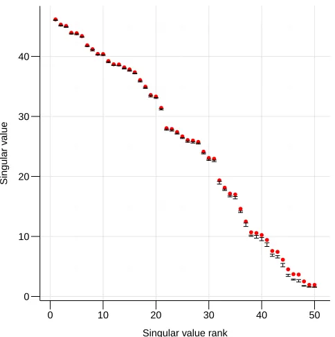
the rank-ordered singular values for a fixed matrix as well as the distribution of the singular values computed via various runs of the ARSVD, an interesting observation is that the estimates are biased for small singular values (Figure 1). Data were generated fromn = 1,000andp = 1,000with true rankd∗ = 50. For the smallest singular values, ARSVD tends to underestimate the singular values, and the standard error is larger. This bias can be considered a form of regularization that shrinks directions corresponding to small singular values. We will discuss this property further in Section 4.1.4.

● ● ●

● ●_●

● ●

● ● ●

● ● ● ●_●

● ●

● ●

●

● ●_● ●

● ● ● ●

● ●

● ●

● ●

●

●

● ● ● ●

● ● ●

● ● ●

●_{● ●}

0 10 20 30 40

0 10 20 30 40 50

Singular value rank

Singular v

alue

Figure 1: Singular value accuracy of ARSVD.Simulation results comparing estimation accuracy of singular values for ARSVD versus SVD on pseudo-random matrices of dimension

n= 1,000andp= 1,000. The exact singular values are in red and confidence intervals for the singular values computed using ARSVD are in blue.

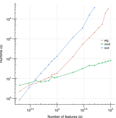
We can compare the runtime of randomized SVD (RSVD) to two standard spectral decomposi-tions methods. We denote the singular value decomposition of a data matrixXas SVD. We denote as eig the procedure first computing Σ =b XXT and then computing the spectral decomposition

ofΣb. For this simulation, we generate pseudo-random matrices that aren×psuch thatn = ₁₀p.

● ●

● ●

● ●

● ●● ●

● ●

● ●

● ●

●

100

101

102 103 104

103.5 ₁₀4 ₁₀4.5 ₁₀5

Number of features (p)

Runtime (s)

● _eig rsvd svd

Figure 2: Comparison of three spectral methods.We compare RSVD, SVD, and eig. The x-axis indexes matrix size aspand the y-axis is the runtime in seconds. Both axes are on a log scale.

A natural question is whether the randomization offers any advantage over well developed effi-cient methods, such as Lanczos-Krylov Subspace estimation, which also operate on the data matrix only through matrix multiplies (Saad, 1992; Lehoucq et al., 1998; Stewart, 2001; Baglama and Reichel, 2006). These subspace methods are also iterative in nature, with the runtime complexity typically scaling asO(qnp), whereq is small. We compare the runtime ratio of our RSVD with a state-of-the-art low-rank approximation algorithm, the blocked Lanczos method implemented in the CRAN packageirlba(Baglama and Reichel, 2006). Data were generated fromn= 1000and

p = 1000with true rankd∗ = 50, and we variedtin ARSVD. We ran both ARSVD and blocked

Lanczos until the Frobenius norm reconstruction error to the original matrix was equal to one degree of precision. We report the ratio of the runtime of ARSVD over blocked Lanczos computed on ten simulated data sets (Table 2). The relative runtime remains approximately constant with simultane-ous increase in both data dimensions, which suggests similar order of complexity for both methods when the latent rank of the data (d∗) is supplied as a static parameter to each method. The relative runtime decreases exponentially when using ARSVD to dynamically estimate the latent rank versus using Bi-Cross-Validation to dynamically estimate the rank supplied to block Lanczos.

n + p 6,000 7,500 9,000 10,500 12,000 relative time

(static rank)

2.5±0.05 1.84±0.03 1.82±0.03 1.83±0.02 1.84±0.04

n + p 2,000 3,500 5,000 6,500 8,000

relative time (dynamic rank)

3.49±1.10 0.58±0.26 0.46±0.21 0.04±0.01 0.25±0.11

Table 2: Runtime ratio of ARSVD versus block Lanczos. We report the sample mean and stan-dard error of ARSVD over block Lanczos based on ten random replicate data sets across dimensionalityn+p.nis incremented by500andpis incremented by1,000. In the static rank experiments, the latent rankd∗ is supplied as a static parameter to both methods. In the dynamic rank experiments, ARSVD estimates the latent rank using the algorithm pre-viously described, and we use Bi-Cross-Validation to dynamically estimate the latent rank supplied to block Lanczos. ARSVD is run for as many iterations as needed until the sam-ple error is equal to within one degree of precision, thus we do not dynamically estimate the number of power iterations,t∗, in these experiments.

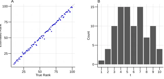
two different signal-to-noise scenarios (Figure 3). In both scenarios, the rank estimates agreed with the true rank values. If the signal-to-noise ratio is low, then our procedure slightly underestimates the rank. We suspect this underestimate is due to the fact that the few smallest variance signal directions tend to be difficult to distinguish from the random noise and hence are less stable under random projections. Our approach tends to select small values fort∗, especially when there is a clear separation between the signal and the noise.

● ●●●

●● ● ●●●

●●● ● ●●●●

●● ●●

● ●●

●● ● ● ●●●

●●

●● ●●●

●●● ●●

● ●●

● ●●●●

●●● ● ● ●

● ●●●●●●

●● ●●●

● ●●

● ●●

●● ●●

●●●● ●● ●●

●●●

25 50 75 100

25 50 75 100

True Rank

Estimated Rank

A

0 5 10 15

8 2 3 4 5 7 9 10

1 6

t

Count

B

Figure 3: Rank estimation of ARSVD.Rank estimation results after performing ARSVD on50

pseudo-random matrices of dimensionn = 10000andp = 10000, with true rankd∗ iid∼ Uniform[10,50]. Matrices are generated as described in Section 4.1.1. Panel A: True rank (d∗) on the x-axis, and estimated rank (dˆ∗) on the y-axis. Panel B: estimations oft∗

4.1.4 LATENTPOPULATIONSTRUCTURE

We examine how accurately ARSVD can be used to correct latent or cryptic population structure. Specifically, we compared the performance of an LMM using ARSVD versus a standard LMM. We simulated genotype and phenotype data where the genotypes have latent population structure that, once corrected for, there remains no association between genotype and phenotype. In other words, the phenotype is conditionally independent of the genotype given the latent (population) structure. This relation is sometimes called the confounding effect of cryptic structure in genomic data, and motivates the need for LMMs in genome-wide studies. Given that simulations are entirely under the null hypothesis of no association between genotype and phenotype, p-values should follow a uniform distribution if the random effect controls population structure appropriately. We consider any result exceeding anα-threshold a false positive, occurring at rateα.

We use the model stated in Mimno et al. (2014) to simulate admixed genotypes withKancestral populations. The genotype of an individual is generated by the following hierarchical model

θi ∼ DirK(α),

φk ∼ Beta(1,1), k= 1, ..., K,

(z1,ij, z2,ij) ∼

Mult(θi),Mult(θi)

forj= 1, ..., p

(x1,ij, x2,ij) ∼

Bin(φz1,ij),Bin(φz2,ij)

forj= 1, ..., p.

The first step samples the the admixture proportions for individuali. The second step samples the allele frequency distribution for populationsk = 1, . . . , K. The third step samples the population of origin for both allele copies over all loci, j = 1, . . . , p. The final step samples both copies of the alleles at each locus j. We generated the phenotype using the following relation: yi ∼ Be(0.5θk+ 0.1(1−θk)).

We looked at four simulation settings n = p = 1000,n = p = 5000,n = 1000, p = 5000,

andn= 5000, p= 1000. Using the p-values for a LMM using ARSVD with the rank parameter

d∗ of the ARSVD specified, we see that the standard LMM is recovered in the limit of d∗ = p

(Figure 4). Of these settings, the case wheren= 1000, p= 5000is the most similar to the standard genomics case where the number of SNPspis much larger than the number of observationsn. A summary of these simulation results is that the ARSVD method is much faster than the standard LMM and performs similarly with respect to correcting for population structure and controlling false positives. We observed that, for the simulation withn= 1000, p= 5000, using ARSVD leads to a substantial reduction of computational complexity with similar performance. In general, we expect the tradeoff between computational efficiency and accuracy to depend on the data. In the case of structured genomic data, we report in these simulations and in Section 4.1.4 that massive computational savings are accompanied by numerical accuracy.

4.2 Association Mapping in Large Genomic Data

● ● ● ● ● ● ● ● ● ● ● ● ● ● ● ● ● ● ● ● ● ● ● ● ● ● ● ● ● ● ● ● ● ● ● ● ● ● ● ● ● ● ● ● ● ● ● ● ● ● ● ● ● ● ● ● ● ● ● ● ● ● ● ● ● ● ● ● ● ● ● ● ● ● ● ● ● ● ● ● ● ● ● ● ● ● ● ● ● ● ● ● ● ● ● ● ● ● ● ● ● ● ● ● ● ● ● ● ● ● ● ● ● ● ● ● ● ● ● ● ● ● ● ● ● ● ● ● ● ● ● ● ● ● ● ● ● ● ● ● ● ● ● ● ● ● ● ● ● ● ● ● ● ● ● ● ● ● ● ● ● ● ● ● ● ● ● ● ● ● ● ● ● ● ● ● ● ● ● ● ● ● ● ● ● ● ● ● ● ● ● ● ● ● ● ● ● ● ● ● ● ● ● ● ● ● ● ● ● ● ● ● ● ● ● ● ● ● ● ● ● ● ● ● ● ● ● ● ● ● ● ● ● ● ● ● ● ● ● ● ● ● ● ● ● ● ● ● ● ● ● ● ● ● ● ● ● ● ● ● ● ● ● ● ● ● ● ● ● ● ● ● ● ● ● ● ● ● ● ● ● ● ● ● ● ● ● ● ● ● ● ● ● ● ● ● ● ● ● ● ● ● ● ● ● ● ● ● ● ● ● ● ● ● ● ● ● ● ● ● ● ● ● ● ● ● ● ● ● ● ● ● ● ● ● ● ● ● ● ● ● ● ● ● ● ● ● ● ● ● ● ● ● ● ● ● ● ● ● ● ● ● ● ● ● ● ● ● ● ● ● ● ● ● ● ● ● ● ● ● ● ● ● ● ● ● ● ● ● ● ● ● ● ● ● ● ● ● ● ● ● ● ● ● ● ● ● ● ● ● ● ● ● ● ● ● ● ● ● ● ● ● ● ● ● ● ● ● ● ● ● ● ● ● ● ● ● ● ● ● ● ● ● ● ● ● ● ● ● ● ● ● ● ● ● ● ● ● ● ● ● ● ● ● ● ● ● ● ● ● ● ● ● ● ● ● ● ● ● ● ● ● ● ● ● ● ● ● ● ● ● ● ● ● ● ● ● ● ● ● ● ● ● ● ● ● ● ● ● ● ● ● ● ● ● ● ● ● ● ● ● ● ● ● ● ● ● ● ● ● ● ● ● ● ● ● ● ● ● ● ● ● ● ● ● ● ● ● ● ● ● ● ● ● ● ● ● ● ● ● ● ● ● ● ● ● ● ● ● ● ● ● ● ● ● ● ● ● ● ● ● ● ● ● ● ● ● ● ● ● ● ● ● ● ● ● ● ● ● ● ● ● ● ● ● ● ● ● ● ● ● ● ● ● ● ● ● ● ● ● ● ● ● ● ● ● ● ● ● ● ● ● ● ● ● ● ● ● ● ● ● ● ● ● ● ● ● ● ● ● ● ● ● ● ● ● ● ● ● ● ● ● ● ● ● ● ● ● ● ● ● ● ● ● ● ● ● ● ● ● ● ● ● ● ● ● ● ● ● ● ● ● ● ● ● ● ● ● ● ● ● ● ● ● ● ● ● ● ● ● ● ● ● ● ● ● ● ● ● ● ● ● ● ● ● ● ● ● ● ● ● ● ● ● ● ● ● ● ● ● ● ● ● ● ● ● ● ● ● ● ● ● ● ● ● ● ● ● ● ● ● ● ● ● ● ● ● ● ● ● ● ● ● ● ● ● ● ● ● ● ● ● ● ● ● ● ● ● ● ● ● ● ● ● ● ● ● ● ● ● ● ● ● ● ● ● ● ● ● ● ● ● ● ● ● ● ● ● ● ● ● ● ● ● ● ● ● ● ● ● ● ● ● ● ● ● ● ● ● ● ● ● ● ● ● ● ● ● ● ● ● ● ● ● ● ● ● ● ● ● ● ● ● ● ● ● ● ● ● ● ● ● ● ● ● ● ● ● ● ● ● ● ● ● ● ● ● ● ● ● ● ● ● ● ● ● ● ● ● ● ● ● ● ● ● ● ● ● ● ● ● ● ● ● ● ● ● ● ● ● ● ● ● ● ● ● ● ● ● ● ● ● ● ● ● ● ● ● ● ● ● ● ● ● ● ● ● ● ● ● ● ● ● ● ● ● ● ● ● ● ● ● ● ● ● ● ● ● ● ● ● ● ● ● ● ● ● ● ● ● ● ● ● ● ● ● ● ● ● ● ● ● ● ● ● ● ● ● ● ● ● ● ● ● ● ● ● ● ● ● ● ● ● ● ● ● ● ● ● ● ● ● ● ● ● ● ● ● ● ● ● ● ● ● ● ● ● ● ● ● ● ● ● ● ● ● ● ● ● ● ● ● ● ● ● ● ● ● ● ● ● ● ● ● ● ● ● ● ● ● ● ● ● ● ● ● ● ● ● ● ● ● ● ● ● ● ● ● ● ● ● ● ● ● ● ● ● ● ● ● ● ● ● ● ● ● ● ● ● ● ● ● ● ● ● ● ● ● ● ● ● ● ● ● ● ● ● ● ● ● ● ● ● ● ● ● ● ● ● ● ● ● ● ● ● ● ● ● ● ● ● ● ● ● ● ● ● ● ● ● ● ● ● ● ● ● ● ● ● ● ● ● ● ● ● ● ● ● ● ● ● ● ● ● ● ● ● ● ● ● ● ● ● ● ● ● ● ● ● ● ● ● ● ● ● ● ● ● ● ● ● ● ● ● ● ● ● ● ● ● ● ● ● ● ● ● ● ● ● ● ● ● ● ● ● ● ● ● ● ● ● ● ● ● ● ● ● ● ● ● ● ● ● ● ● ● ● ● ● ● ● ● ● ● ● ● ● ● ● ● ● ● ● ● ● ● ● ● ● ● ● ● ● ● ● ● ● ● ● ● ● ● ● ● ● ● ● ● ● ● ● ● ● ● ● ● ● ● ● ● ● ● ● ● ● ● ● ● ● ● ● ● ● ● ● ● ● ● ● ● ● ● ● ● ● ● ● ● ● ● ● ● ● ● ● ● ● ● ● ● ● ● ● ● ● ● ● ● ● ● ● ● ● ● ● ● ● ● ● ● ● ● ● ● ● ● ● ● ● ● ● ● ● ● ● ● ● ● ● ● ● ● ● ● ● ● ● ● ● ● ● ● ● ● ● ● ● ● ● ● ● ● ● ● ● ● ● ● ● ● ● ● ● ● ● ● ● ● ● ● ● ● ● ● ● ● ● ● ● ● ● ● ● ● ● ● ● ● ● ● ● ● ● ● ● ● ● ● ● ● ● ● ● ● ● ● ● ● ● ● ● ● ● ● ● ● ● ● ● ● ● ● ● ● ● ● ● ● ● ● ● ● ● ● ● ● ● ● ● ● ● ● ● ● ● ● ● ● ● ● ● ● ● ● ● ● ● ● ● ● ● ● ● ● ● ● ● ● ● ● ● ● ● ● ● ● ● ● ● ● ● ● ● ● ● ● ● ● ● ● ● ● ● ● ● ● ● ● ● ● ● ● ● ● ● ● ● ● ● ● ● ● ● ● ● ● ● ● ● ● ● ● ● ● ● ● ● ● ● ● ● ● ● ● ● ● ● ● ● ● ● ● ● ● ● ● ● ● ● ● ● ● ● ● ● ● ● ● ● ● ● ● ● ● ● ● ● ● ● ● ● ● ● ● ● ● ● ● ● ● ● ● ● ● ● ● ● ● ● ● ● ● ● ● ● ● ● ● ● ● ● ● ● ● ● ● ● ● ● ● ● ● ● ● ● ● ● ● ● ● ● ● ● ● ● ● ● ● ● ● ● ● ● ● ● ● ● ● ● ● ● ● ● ● ● ● ● ● ● ● ● ● ● ● ● ● ● ● ● ● ● ● ● ● ● ● ● ● ● ● ● ● ● ● ● ● ● ● ● ● ● ● ● ● ● ● ● ● ● ● ● ● ● ● ● ● ● ● ● ● ● ● ● ● ● ● ● ● ● ● ● ● ● ● ● ● ● ● ● ● ● ● ● ● ● ● ● ● ● ● ● ● ● ● ● ● ● ● ● ● ● ● ● ● ● ● ● ● ● ● ● ● ● ● ● ● ● ● ● ● ● ● ● ● ● ● ● ● ● ● ● ● ● ● ● ● ● ● ● ● ● ● ● ● ● ● ● ● ● ● ● ● ● ● ● ● ● ● ● ● ● ● ● ● ● ● ● ● ● ● ● ● ● ● ● ● ● ● ● ● ● ● ● ● ● ● ● ● ● ● ● ● ● ● ● ● ● ● ● ● ● ● ● ● ● ● ● ● ● ● ● ● ● ● ● ● ● ● ● ● ● ● ● ● ● ● ● ● ● ● ● ● ● ● ● ● ● ● ● ● ● ● ● ● ● ● ● ● ● ● ● ● ● ● ● ● ● ● ● ● ● ● ● ● ● ● ● ● ● ● ● ● ● ● ● ● ● ● ● ● ● ● ● ● ● ● ● ● ● ● ● ● ● ● ● ● ● ● ● ● ● ● ● ● ● ● ● ● ● ● ● ● ● ● ● ● ● ● ● ● ● ● ● ● ● ● ● ● ● ● ● ● ● ● ● ● ● ● ● ● ● ● ● ● ● ● ● ● ● ● ● ● ● ● ● ● ● ● ● ● ● ● ● ● ● ● ● ● ● ● ● ● ● ● ● ● ● ● ● ● ● ● ● ● ● ● ● ● ● ● ● ● ● ● ● ● ● ● ● ● ● ● ● ● ● ● ● ● ● ● ● ● ● ● ● ● ● ● ● ● ● ● ● ● ● ● ● ● ● ● ● ● ● ● ● ● ● ● ● ● ● ● ● ● ● ● ● ● ● ● ● ● ● ● ● ● ● ● ● ● ● ● ● ● ● ● ● ● ● ● ● ● ● ● ● ● ● ● ● ● ● ● ● ● ● ● ● ● ● ● ● ● ● ● ● ● ● ● ● ● ● ● ● ● ● ● ● ● ● ● ● ● ● ● ● ● ● ● ● ● ● ● ● ● ● ● ● ● ● ● ● ● ● ● ● ● ● ● ● ● ● ● ● ● ● ● ● ● ● ● ● ● ● ● ● ● ● ● ● ● ● ● ● ● ● ● ● ● ● ● ● ● ● ● ● ● ● ● ● ● ● ● ● ● ● ● ● ● ● ● ● ● ● ● ● ● ● ● ● ● ● ● ● ● ● ● ● ● ● ● ● ● ● ● ● ● ● ● ● ● ● ● ● ● ● ● ● ● ● ● ● ● ● ● ● ● ● ● ● ● ● ● ● ● ● ● ● ● ● ● ● ● ● ● ● ● ● ● ● ● ● ● ● ● ● ● ● ● ● ● ● ● ● ● ● ● ● ● ● ● ● ● ● ● ● ● ● ● ● ● ● ● ● ● ● ● ● ● ● ● ● ● ● ● ● ● ● ● ● ● ● ● ● ● ● ● ● ● ● ● ● ● ● ● ● ● ● ● ● ● ● ● ● ● ● ● ● ● ● ● ● ● ● ● ● ● ● ● ● ● ● ● ● ● ● ● ● ● ● ● ● ● ● ● ● ● ● ● ● ● ● ● ● ● ● ● ● ● ● ● ● ● ● ● ● ● ● ● ● ● ● ● ● ● ● ● ● ● ● ● ● ● ● ● ● ● ● ● ● ● ● ● ● ● ● ● ● ● ● ● ● ● ● ● ● ● ● ● ● ● ● ● ● ● ● ● ● ● ● ● ● ● ● ● ● ● ● ● ● ● ● ● ● ● ● ● ● ● ● ● ● ● ● ● ● ● ● ● ● ● ● ● ● ● ● ● ● ● ● ● ● ● ● ● ● ● ● ● ● ● ● ● ● ● ● ● ● ● ● ● ● ● ● ● ● ● ● ● ● ● ● ● ● ● ● ● ● ● ● ● ● ● ● ● ● ● ● ● ● ● ● ● ● ● ● ● ● ● ● ● ● ● ● ● ● ● ● ● ● ● ● ● ● ● ● ● ● ● ● ● ● ● ● ● ● ● ● ● ● ● ● ● ● ● ● ● ● ● ● ● ● ● ● ● ● ● ● ● ● ● ● ● ● ● ● ● ● ● ● ● ● ● ● ● ● ● ● ● ● ● ● ● ● ● ● ● ● ● ● ● ● ● ● ● ● ● ● ● ● ● ● ● ● ● ● ● ● ● ● ● ● ● ● ● ● ● ● ● ● ● ● ● ● ● ● ● ● ● ● ● ● ● ● ● ● ● ● ● ● ● ● ● ● ● ● ● ● ● ● ● ● ● ● ● ● ● ● ● ● ● ● ● ● ● ● ● ● ● ● ● ● ● ● ● ● ● ● ● ● ● ● ● ● ● ● ● ● ● ● ● ● ● ● ● ● ● ● ● ● ● ● ● ● ● ● ● ● ● ● ● ● ● ● ● ● ● ● ● ● ● ● ● ● ● ● ● ● ● ● ● ● ● ● ● ● ● ● ● ● ● ● ● ● ● ● ● ● ● ● ● ● ● ● ● ● ● ● ● ● ● ● ● ● ● ● ● ● ● ● ● ● ● ● ● ● ● ● ● ● ● ● ● ● ● ● ● ● ● ● ● ● ● ● ● ● ● ● ● ● ● ● ● ● ● ● ● ● ● ● ● ● ● ● ● ● ● ● ● ● ● ● ● ● ● ● ● ● ● ● ● ● ● ● ● ● ● ● ● ● ● ● ● ● ● ● ● ● ● ● ● ● ● ● ● ● ● ● ● ● ● ● ● ● ● ● ● ● ● ● ● ● ● ● ● ● ● ● ● ● ● ● ● ● ● ● ● ● ● ● ● ● ● ● ● ● ● ● ● ● ● ● ● ● ● ● ● ● ● ● ● ● ● ● ● ● ● ● ● ● ● ● ● ● ● ● ● ● ● ● ● ● ● ● ● ● ● ● ● ● ● ● ● ● ● ● ● ● ● ● ● ● ● ● ● ● ● ● ● ● ● ● ● ● ● ● ● ● ● ● ● ● ● ● ● ● ● ● ● ● ● ● ● ● ● ● ● ● ● ● ● ● ● ● ● ● ● ● ● ● ● ● ● ● ● ● ● ● ● ● ● ● ● ● ● ● ● ● ● ● ● ● ● ● ● ● ● ● ● ● ● ● ● ● ● ● ● ● ● ● ● ● ● ● ● ● ● ● ● ● ● ● ● ● ● ● ● ● ● ● ● ● ● ● ● ● ● ● ● ● ● ● ● ● ● ● ● ● ● ● ● ● ● ● ● ● ● ● ● ● ● ● ● ● ● ● ● ● ● ● ● ● ● ● ● ● ● ● ● ● ● ● ● ● ● ● ● ● ● ● ● ● ● ● ● ● ● ● ● ● ● ● ● ● ● ● ● ● ● ● ● ● ● ● ● ● ● ● ● ● ● ● ● ● ● ● ● ● ● ● ● ● ● ● ● ● ● ● ● ● ● ● ● ● ● ● ● ● ● ● ● ● ● ● ● ● ● ● ● ● ● ● ● ● ● ● ● ● ● ● ● ● ● ● ● ● ● ● ● ● ● ● ● ● ● ● ● ● ● ● ● ● ● ● ● ● ● ● ● ● ● ● ● ● ● ● ● ● ● ● ● ● ● ● ● ● ● ● ● ● ● ● ● ● ● ● ● ● ● ● ● ● ● ● ● ● ● ● ● ● ● ● ● ● ● ● ● ● ● ● ● ● ● ● ● ● ● ● ● ● ● ● ● ● ● ● ● ● ● ● ● ● ● ● ● ● ● ● ● ● ● ● ● ● ● ● ● ● ● ● ● ● ● ● ● ● ● ● ● ● ● ● ● ● ● ● ● ● ● ● ● ● ● ● ● ● ● ● ● ● ● ● ● ● ● ● ● ● ● ● ● ● ● ● ● ● ● ● ● ● ● ● ● ● ● ● ● ● ● ● ● ● ● ● ● ● ● ● ● ● ● ● ● ● ● ● ● ● ● ● ● ● ● ● ● ● ● ● ● ● ● ● ● ● ● ● ● ● ● ● ● ● ● ● ● ● ● ● ● ● ● ● ● ● ● ● ● ● ● ● ● ● ● ● ● ● ● ● ● ● ● ● ● ● ● ● ● ● ● ● ● ● ● ● ● ● ● ● ● ● ● ● ● ● ● ● ● ● ● ● ● ● ● ● ● ● ● ● ● ● ● ● ● ● ● ● ● ● ● ● ● ● ● ● ● ● ● ● ● ● ● ● ● ● ● ● ● ● ● ● ● ● ● ● ● ● ● ● ● ● ● ● ● ● ● ● ● ● ● ● ● ● ● ● ● ● ● ● ● ● ● ● ● ● ● ● ● ● ● ● ● ● ● ● ● ● ● ● ● ● ● ● ● ● ● ● ● ● ● ● ● ● ● ● ● ● ● ● ● ● ● ● ● ● ● ● ● ● ● ● ● ● ● ● ● ● ● ● ● ● ● ● ● ● ● ● ● ● ● ● ● ● ● ● ● ● ● ● ● ● ● ● ● ● ● ● ● ● ● ● ● ● ● ● ● ● ● ● ● ● ● ● ● ● ● ● ● ● ● ● ● ● ● ● ● ● ● ● ● ● ● ● ● ● ● ● ● ● ● ● ● ● ● ● ● ● ● ● ● ● ● ● ● ● ● ● ● ● ● ● ● ● ● ● ● ● ● ● ● ● ● ● ● ● ● ● ● ● ● ● ● ● ● ● ● ● ● ● ● ● ● ● ● ● ● ● ● ● ● ● ● ● ● ● ● ● ● ● ● ● ● ● ● ● ● ● ● ● ● ● ● ● ● ● ● ● ● ● ● ● ● ● ● ● ● ● ● ● ● ● ● ● ● ● ● ● ● ● ● ● ● ● ● ● ● ● ● ● ● ● ● ● ● ● ● ● ● ● ● ● ● ● ● ● ● ● ● ● ● ● ● ● ● ● ● ● ● ● ● ● ● ● ● ● ● ● ● ● ● ● ● ● ● ● ● ● ● ● ● ● ● ● ● ● ● ● ●

n = 1,000 p = 1,000 n = 1,000 p = 5,000

n = 5,000 p = 1,000 n = 5,000 p = 5,000 0.00 0.25 0.50 0.75 1.00 0.00 0.25 0.50 0.75 1.00 0.00 0.25 0.50 0.75 1.00 0.00 0.25 0.50 0.75 1.00

10 100 200 300 400 500 600 700 800 900 1000 10 500 1000 1500 2000 2500 3000 3500 4000 4500 5000

10 100 200 300 400 500 600 700 800 900 1000 10 500 1000 1500 2000 2500 3000 3500 4000 4500 5000

Rank

P

−

V

alue

Fraction False Positives 0.0086 0.009 0.016 0.0162 0.0176 0.018 0.0198 0.021 0.03 0.0314 0.042 0.045 0.062 0.068 0.0722 0.1042 0.106 0.1622 0.167 0.2452 0.25 0.275 0.311 0.343 0.396 0.41 0.412 0.418 0.452 0.516 0.611 0.729 0.816 0.82 0.9144 0.919

Figure 4: Controlling for structure. RSVD with pylmm is applied to four simulation settings with varyingnandp. The x-axis is the setting of the ARSVD parameterd∗. The y-axis corresponds to the p-values from the LMM for each of thepfeatures. The color of each box plot represents the fraction of false positive rate of the LMM using ARSVD.

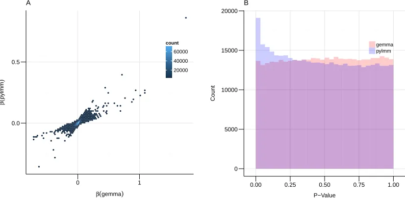
association studies. Our LMM with ARSVD procedure uses EMMAX (pylmm) to solve the LMM. The two methods we compared to are EMMAX with the addition of ARSVD and GEMMA (Zhou et al., 2013) (GEMMA is executed with the-lmmoption to most closely approximate the analysis that pylmm performs).

ARSVD on the whole genome took 82.2 seconds, while a traditional eigendecomposition of the covariance matrix in pylmm took 88 mins 23.9 seconds. In order to most accurately control for the test statistic computed in a LMM and to achieve maximal statistical power, it is suggested that a covariance matrix is constructed once per (22) chromosomes, performed by holding out the test chromosome and concatenating the remaining chromosomes (Yang et al., 2014). Our method performs the 22 decompositions in a total of 5 mins 4.8 secs, while the traditional decomposition method takes 4 hrs 24 mins.

of β for pylmm and GEMMA are strongly correlated. The distributions of p-values computed by pylmm show enrichment in low p-values. This suggests that the regularization in pylmm may capture additional associations.

0.0 0.5

0 1

β(gemma)

β

(

p

y

lm

m

)

20000 40000 60000 count A

0 5000 10000 15000 20000

0.00 0.25 0.50 0.75 1.00

P−Value

Count

gemma pylmm B

Figure 5: Comparison of pylmm and GEMMA.A) A scatter plot of theβ-values for GEMMA on the x-axis versus theβ-values for pylmm on the y-axis. B) Histogram of p-values for both methods, GEMMA in red and pylmm in blue.

We compared the most significant associations that we identified to results from other analyses of Crohn’s disease. One source of associations is from a large-scale meta-analysis of Crohn’s disease consisting of 6,333 affected individuals (cases) and 15,056 controls, and the top association signals were followed up on in 15,694 cases, 14,026 controls, and 414 parent-offspring trios (Franke et al., 2010). We denote this list as MA. In Listgarten et al. (2012), the list of associated genetic variants collected includes the MA list as well as the WTCCC list. The major histocompatibility complex (MHC) is a region that has been previously associated to Crohn’s disease and autoimmune disease in general. We denote the list of variants in this region as MHC. We report the overlap between the results obtained from our method to the MA list, the union of the WTCCC and MA lists, and the union of the WTCCC, MA, and MHC lists. (Table 3). We select our top hits using two cutoffs: the top 0.5% with respect to negative log p-value, and the associations that pass a local false discovery rate (LFDR) of 5% (Strimmer, 2008).