Katyusha: The First Direct Acceleration of
Stochastic Gradient Methods
Zeyuan Allen-Zhu∗ [email protected]
Microsoft Research AI Redmond, WA 98052, USA
Editor:Leon Bottou
Abstract
Nesterov’s momentum trick is famously known for accelerating gradient descent, and has been proven useful in building fast iterative algorithms. However, in the stochastic setting, counterexamples exist and prevent Nesterov’s momentum from providing similar accelera-tion, even if the underlying problem is convex and finite-sum.
We introduce Katyusha, a direct, primal-only stochastic gradient method to fix this issue. In convex finite-sum stochastic optimization, Katyushahas an optimal accelerated convergence rate, and enjoys an optimal parallel linear speedup in the mini-batch setting. The main ingredient isKatyusha momentum, a novel “negative momentum” on top of Nesterov’s momentum. It can be incorporated into a variance-reduction based algorithm and speed it up, both in terms of sequential and parallel performance. Since variance reduction has been successfully applied to a growing list of practical problems, our paper suggests that in each of such cases, one could potentially try to give Katyusha a hug.
1. Introduction
In large-scale machine learning, the number of data examples is usually very large. To search
for the optimal solution, one often uses stochastic gradient methods which only require one
(or a small batch of) random example(s) per iteration in order to form anestimator of the
full gradient.
While full-gradient based methods can enjoy an accelerated (and optimal) convergence
rate if Nesterov’s momentum trick is used (Nesterov, 1983, 2004, 2005), theory for stochastic gradient methods are generally lagging behind and less is known for their acceleration.
At a high level, momentum is dangerous if stochastic gradients are present. If some
gradient estimator is very inaccurate, then adding it to the momentum and moving further in this direction (for every future iteration) may hurt the convergence performance. In other words, when naively equipped with momentum, stochastic gradient methods are “very prune
to error accumulation” (Koneˇcn`y et al., 2016) and donotyield accelerated convergence rates
in general.1
∗. The arXiv version of this paper can be found athttp://arxiv.org/abs/1603.05953, and may include future revisions.
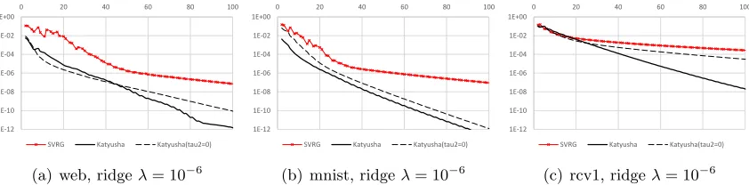
1. In practice, experimentalists have observed that momentums could sometimes help if stochastic gradient iterations are used. However, the so-obtained methods (1) sometimes fail to converge in an accelerated rate, (2) become unstable and hard to tune, and (3) have no support theory behind them. See Section 7.1 for an experiment illustrating that, even for convex stochastic optimization.
c
In this paper, we show that at least for convex optimization purposes, such an issue can be solved with a novel “negative momentum” that can be added on top of momentum. We obtain accelerated and the first optimal convergence rates for stochastic gradient methods. As one of our side results, under this “negative momenmtum,” our new method enjoys a linear speedup in the parallel (i.e., mini-match) setting. We hope our new insight could potentially deepen our understanding to the theory of accelerated methods.
Problem Definition. Consider the following composite convex minimization problem
min
x∈Rd
n
F(x)def=f(x) +ψ(x)def= 1
n n X
i=1
fi(x) +ψ(x) o
. (1.1)
Here,f(x) = 1nPn
i=1fi(x) is a convex function that is a finite average ofnconvex, smooth
functions fi(x), and ψ(x) is convex, lower semicontinuous (but possibly non-differentiable)
function, sometimes referred to as the proximal function. We mostly focus on the case
when ψ(x) is σ-strongly convex and eachfi(x) is L-smooth. (Both these assumptions can
be removed and we shall discuss that later.) We look for approximate minimizers x∈ Rd
satisfying F(x)≤F(x∗) +ε, where x∗ ∈arg minx{F(x)}.
Problem (1.1) arises in many places in machine learning, statistics, and operations
re-search. All convexregularized empirical risk minimization (ERM) problems such as Lasso,
SVM, Logistic Regression, fall into this category (see Section 1.3). Efficient stochastic meth-ods for Problem (1.1) have also inspired stochastic algorithms for neural nets (Johnson and Zhang, 2013; Allen-Zhu and Hazan, 2016a; Lei et al., 2017) as well as SVD, PCA, and CCA (Garber et al., 2016; Allen-Zhu and Li, 2016, 2017b).
We summarize the history of stochastic gradient methods for Problem (1.1) in three eras.
The First Era: Stochastic Gradient Descent (SGD).
Recall that stochastic gradient methods iteratively perform the following update
stochastic gradient iteration: xk+1←arg min
y∈Rd
n 1
2ηky−xkk
2
2+h∇ek, yi+ψ(y) o
,
where η is the step length and ∇ek is a random vector satisfying E[∇ek] = ∇f(xk) and
is referred to as the gradient estimator. If the proximal function ψ(y) equals zero, the
update reduces to xk+1 ←xk−η∇ek. A popular choice for the gradient estimator is to set
e
∇k=∇fi(xk) for some random indexi∈[n] per iteration, and methods based on this choice
are known as stochastic gradient descent (SGD) (Zhang, 2004; Bottou). Since computing
∇fi(x) is usually n times faster than that of ∇f(x), SGD enjoys a low per-iteration cost
as compared to full-gradient methods; however, SGD cannot converge at a rate faster than
The Second Era: Variance Reduction Gives Faster Convergence.
The convergence rate of SGD can be further improved with the so-called
variance-reductiontechnique, first proposed by Schmidt et al. (2013) (solving a sub-case of Problem (1.1)) and then followed by many others (Zhang et al., 2013; Mahdavi et al., 2013; Johnson and Zhang, 2013; Shalev-Shwartz and Zhang, 2013; Shalev-Shwartz, 2016; Shalev-Shwartz and Zhang, 2012; Xiao and Zhang, 2014; Defazio et al., 2014; Mairal, 2015; Allen-Zhu and Yuan, 2016). In these cited results, the authors have shown that SGD converges much faster if
one makes a better choice of the gradient estimator∇ekso that its variance reduces as k
in-creases. One way to choose this estimator can be described as follows (Johnson and Zhang,
2013; Zhang et al., 2013). Keep a snapshot vector xe = xk that is updated once every m
iterations (where m is some parameter usually around 2n), and compute the full gradient
∇f(ex) only for such snapshots. Then, set
e
∇k =∇fi(xk)− ∇fi(xe) +∇f(ex) . (1.2)
This choice of gradient estimator ensures that its variance approaches to zero as k
grows. Furthermore, the number of stochastic gradients (i.e., the number of computations
of ∇fi(x) for some i) required to reach an ε-approximate minimizer of Problem (1.1) is
only O n+Lσlog1ε. Since it is often denoted by κ def= L/σ the condition number of the
problem, we rewrite the above iteration complexity asO (n+κ) log1ε.
Unfortunately, the iteration complexities of all known variance-reduction based
meth-ods have a linear dependence on κ. It was an open question regarding how to obtain an
accelerated stochastic gradient method with an optimal√κ dependency.
The Third Era: Acceleration Gives Fastest Convergence.
This open question was partially solved recently by the APPA (Frostig et al., 2015) and Catalyst (Lin et al., 2015) reductions, both based on an outer-inner loop structure first proposed by Shalev-Shwartz and Zhang (2014). We refer to both of them as Catalyst in
this paper. Catalyst solves Problem (1.1) usingO n+√nκlogκlog1εstochastic gradient
iterations, through a logarithmic number of calls to a variance-reduction method.2 However,
Catalyst is still imperfect for the following reasons:
• Optimality. Catalyst does not match the optimal √κ dependence (Woodworth and
Srebro, 2016) and has an extra logκ factor. It yields suboptimal rate logT42T if the
objec-tive is not strongly convex or is non-smooth; and it yields suboptimal rate logT4T if the
objective is both non-strongly convex and non-smooth.3
• Practicality. To the best of our knowledge, Catalyst is not very practical since each of its inner iterations needs to be very accurately executed. This makes the stopping cri-terion hard to be tuned, and makes Catalyst sometimes run slower than non-accelerated variance-reduction methods. We have also confirmed this in our experiments.
• Parallelism. To the best of our knowledge, Catalyst does not give competent parallel
performance (see Section 1.2). If b ∈ {1, . . . , n} stochastic gradients (instead of one)
are computed in each iteration, the number of iterations of Catalyst reduces by O(√b).
2. Note thatn+√nκis always less thanO(n+κ).
In contrast, the best parallel speedup one can hope for is “linear speedup”: that is, to
reduce the number of iterations by a factor ofO(b) forb≤√n.
• Generality. To the best of our knowledge, being a reduction-based method, Catalyst does not seem to support non-Euclidean norm smoothness (see Section 1.2).
Another acceleration method by Lan and Zhou (2015) is based on a primal-dual analysis
that also has suboptimal convergence rates like Catalyst. Their method requires n times
more storage compared with Catalyst for solving Problem (1.1).
In sum, it is desirable and also an open question to develop a direct, primal-only, and
optimal accelerated stochastic gradient method without using reductions. This could have both theoretical and practical impacts to the problems that fall into the general framework of (1.1), and potentially deepen our understanding to acceleration in stochastic settings.
1.1 Our Main Results and High-Level Ideas
We develop a direct, accelerated stochastic gradient methodKatyushafor Problem (1.1) in
O n+√nκlog(1/ε) stochastic gradient iterations (see Theorem 2.1).
This gives both optimal dependency on κ and on ε which was not obtained before for
stochastic gradient methods. In addition, ifF(·) is non-strongly convex (non-SC),Katyusha
converges to anε-minimizer in
O nlog(1/ε) +pnL/ε
stochastic gradient iterations (see Corollary 3.7).
This gives an optimal ε ∝ Tn2 rate where in contrast Catalyst has rate ε ∝
nlog4T
T2 . The
lower bound from Woodworth and Srebro (2016) is Ω n+pnL/ε
.
Our Algorithm. If ignoring the proximal termψ(·) and viewing it as zero, ourKatyusha
method iteratively perform the following updates fork= 0,1, . . .:
• xk+1←τ1zk+τ2ex+ (1−τ1−τ2)yk; (soxk+1=yk+τ1(zk−yk) +τ2(ex−yk) )
• ∇ek+1← ∇f(xe) +∇fi(xk+1)− ∇fi(ex) whereiis a random index in [n];
• yk+1 ←xk+1−31L∇ek+1, and
• zk+1←zk−α∇ek+1.
Above, ex is a snapshot point which is updated every m iterations, ∇ek+1 is the gradient
estimator defined in the same way as (1.2), τ1, τ2 ∈ [0,1] are two momentum parameters,
and α is a parameter that is equal to 3τ1
1L. The reason for keeping three vector sequences
(xk, yk, zk) is a common ingredient that can be found in all existing accelerated methods.4
Our New Technique – Katyusha Momentum. The most interesting ingredient of
Katyusha is the novel choice of xk+1 which is a convex combination of yk, zk, and xe.
Our theory suggests the parameter choices τ2 = 0.5 andτ1 = min{
p
nσ/L,0.5} and they work well in practice too. To explain this novel combination, let us recall the classical “momentum” view of accelerated methods.
In a classical accelerated gradient method, xk+1 is only a convex combination of yk
and zk (or equivalently, τ2 = 0 in our formulation). At a high level, zk plays the role of
“momentum” which adds a weighted sum of the gradient history intoyk+1. As an illustrative
example, supposeτ2 = 0,τ1=τ, andx0=y0=z0. Then, one can compute that
yk =
x0−31L∇e1, k= 1;
x0−31L∇e2− (1−τ)31L+τ α
e
∇1, k= 2;
x0−31L∇e3− (1−τ)31L+τ α
e
∇2− (1−τ)2 13L+ (1−(1−τ)2)α e
∇1, k= 3.
Sinceαis usually much larger than 1/3L, the above recursion suggests that the contribution
of a fixed gradient ∇et gradually increases as time goes. For instance, the weight on ∇e1 is
increasing because 31L < (1−τ)31L+τ α< (1−τ)2 13L+ (1−(1−τ)2)α .This is known
as “momentum” which is at the heart of all accelerated first-order methods.
In Katyusha, we put a “magnet” around xe, where we choose xe to be essentially “the
average xt of the most recent n iterations”. Whenever we compute the next xk+1, it will
be attracted by the magnet ex with weight τ2 = 0.5. This is a strong magnet: it ensures
thatxk+1 is not too far away fromxeso the gradient estimator remains “accurate enough”.
This can be viewed as a “negative momentum” component, because the magnet retracts
xk+1 back to ex and this can be understood as “counteracting a fraction of the positive
momentum incurred from earlier iterations.”
We call it the Katyusha momentum.
This summarizes the high-level idea behind our Katyusha method. We remark here if
τ1 = τ2 = 0, Katyusha becomes almost identical to SVRG (Johnson and Zhang, 2013;
Zhang et al., 2013) which is a variance-reduction based method.
1.2 Our Side Results
Parallelism / Mini-batch. Instead of using a single∇fi(·) per iteration, for any
stochas-tic gradient method, one can replace it with the average ofbstochastic gradients1b P
i∈S∇fi(·),
whereS is a random subset of [n] with cardinalityb. This is known as themini-batch
tech-nique and it allows the stochastic gradients to be computed in a distributed manner, using
up to bprocessors.
OurKatyushamethod trivially extends to this mini-batch setting. For instance, at least forb∈ {1,2, . . . ,d√ne},Katyushaenjoys alinear speed-up in the parallel running time. In other words, if ignoring communication overhead,
Katyushacan be distributed tob≤√n machines with a parallel speed-up factorb.
In contrast, to the best of our knowledge, without any additional assumption, (1) non-accelerated methods such as SVRG or SAGA are not known to enjoy any parallel speed-up;
(2) Catalyst enjoys a parallel speed-up factor of only√b. Details are in Section 5.
Non-Uniform Smoothness. If each fi(·) has a possibly different smooth parameter Li
and L = n1Pn
i=1Li, then an naive implementation of Katyusha only gives a complexity
that depends on maxiLi but notL. In such a case, we can select the random indexi∈[n]
Furthermore, suppose f(x) = n1Pn
i=1fi(x) is smooth with parameter L, it satisfies
L ∈ [L, nL]. One can ask whether or not L influences the performance of Katyusha. We
show that, in the mini-batch setting whenbis large, the total complexity becomes a function
on Las opposed to L. The details are in Section 5.
A Precise Statement. Taking into account both the mini-batch parameter b and the
non-uniform smoothness parametersL andL, we showKatyushasolves Problem (1.1) in
O n+bpL/σ+
q nL/σ
·log1
ε
stochastic gradient computations (see Theorem 5.2)
Non-Euclidean Norms. If the smoothness of each fi(x) is with respect to a
non-Euclidean norm (such as the well known`1norm case over the simplex), our main result still
holds. Our update on theyk+1 side becomes the non-Euclidean norm gradient descent, and
our update on thezk+1 side becomes the non-Euclidean norm mirror descent. We include
such details in Section 6. To the best of our knowledge, most known accelerated methods (including Catalyst, AccSDCA and APCG) do not work with non-Euclidean norms. SPDC can be revised to work with non-Euclidean norms, see (Allen-Zhu et al., 2016b).
Remark on Katyusha Momentum Weight τ2. To provide the simplest proof, we
choose τ2 = 1/2 which also works well in practice. Our proof trivially generalizes to all
constant values τ2 ∈ (0,1), and it could be beneficial to tune τ2 for different datasets.
However, for a stronger comparison, in our experiments we refrain from tuning τ2: by
fixing τ2 = 1/2 and without increasing parameter tuning difficulties, Katyusha already
outperforms most of the state-of-the-arts.
In the mini-batch setting, it turns out the best theoretical choice is essentially τ2 = 21b,
where b is the size of the mini-batch. In other words, the larger the mini-batch size, the
smaller weight we want to give to Katyusha momentum. This should be intuitive, because
whenb=nwe are almost in the full-gradient setting and do not need Katyusha momentum.
1.3 Applications: Optimal Rates for Empirical Risk Minimization
Suppose we are given n feature vectors a1, . . . , an ∈ Rd corresponding to n data samples.
Then, theempirical risk minimization (ERM)problem is to study Problem (1.1) when each
fi(x) is “rank-one” structured: fi(x)
def
= gi(hai, xi) for some loss functiongi:R→R. Slightly
abusing notation, we writefi(x) =fi(hai, xi).5 In such a case, Problem (1.1) becomes
ERM: minx∈Rd
n
F(x)def=f(x) +ψ(x)def= 1nPn
i=1fi(hai, xi) +ψ(x) o
. (1.3)
Without loss of generality, we assume each ai has norm 1 because otherwise one can scale
fi(·) accordingly. As summarized for instance in Allen-Zhu and Hazan (2016b), there are
four interesting cases of ERM problems, all can be written in the form of (1.3):
Case 1: ψ(x) isσ-SC and fi(x) isL-smooth. Examples: ridge regression, elastic net;
Case 2: ψ(x) is non-SC andfi(x) isL-smooth. Examples: Lasso, logistic regression;
Case 3: ψ(x) isσ-SC and fi(x) is non-smooth. Examples: support vector machine;
Case 4: ψ(x) is non-SC andfi(x) is non-smooth. Examples: `1-SVM.
Known Results. For all of the four ERM cases above, accelerated stochastic methods were introduced in the literature, most notably AccSDCA (Shalev-Shwartz and Zhang, 2014), APCG (Lin et al., 2014), SPDC (Zhang and Xiao, 2015). These methods have suboptimal convergence rates for Cases 2, 3 and 4. (In fact, they also have the suboptimal dependence on
the condition numberL/σ for Case 1.) The best known rate was log(1√/ε)
ε , log(1√/ε)
ε , or
log(1/ε) ε
respectively for Cases 2, 3, or 4, and is a factor log(1/ε) worse than optimal (Woodworth
and Srebro, 2016).
It is an open question to design a stochastic gradient method with optimal convergence for such problems. In particular, Dang and Lan (2014) provided an interesting attempt to
remove such log factors but using a non-classical notion of convergence.6
Besides the log factor loss in the running time,7 the aforementioned methods suffer from
several other issues that most dual-based methods also suffer. First, they only apply to ERM problems but not to the more general Problem (1.1). Second, they require proximal
updates with respect to the Fenchel conjugatefi∗(·) which is sometimes unpleasant to work
with. Third, their performances cannot benefit from the implicit strong convexity inf(·).
All of these issues together make these methods sometimes even outperformed by primal-only non-accelerated ones, such as SAGA (Defazio et al., 2014) or SVRG (Johnson and Zhang, 2013; Zhang et al., 2013).
Our Results. Katyusha simultaneously closes the gap for all of the three classes of problems with the help from the optimal reductions developed in Allen-Zhu and Hazan
(2016b). We obtain anε-approximate minimizer for Case 2 inO nlog1ε+
√ nL √
ε
iterations,
for Case 3 in O nlog1ε +
√ n √
σε
iterations, and for Case 4 in O nlog1ε +
√ n ε
iterations. None of the existing accelerated methods can lead to such optimal rates even if the optimal reductions are used.
Woodworth and Srebro (2016) proved the tightness of our results. They showed lower
bounds Ω n+
√ nL √
ε
, Ω n+
√ n √
σε
, and Ω n+
√ n ε
for Cases 2, 3, and 4 respectively.8
1.4 Roadmap
• In Section 2, we state and prove our theorem on Katyushafor the strongly convex case.
6. Dang and Lan (2014) work in a primal-dualφ(x, y) formulation of Problem (1.1), and produce a primal-dual pair (x, y) so that for every fixed (u, v), the expectation E[φ(x, v)−φ(u, y)]≤ε. Unfortunately,
to ensurexis anε-approximate minimizer of Problem (1.1), one needs the strongerE[max(u,v)φ(x, v)−
φ(u, y)]≤εto hold.
7. In fact, dual-based methods have to suffer from a log factor loss in the convergence rate. This is so because even for Case 1 of Problem (1.3), converting an ε-maximizer for the dual objective to the primal, one only obtains annκε-minimizer on the primal objective. As a result, algorithms like APCG who directly work on the dual, algorithms like SPDC who maintain both primal and dual variables, and algorithms like RPDG (Lan and Zhou, 2015) that are primal-like but still use dual analysis, have to suffer from a log loss in the convergence rates.
8. More precisely, their lower bounds for Cases 3 and 4 are Ω min1
σε, n+ √
n √
σε and Ω min
1
ε2, n+ √
n ε .
• In Section 3, we apply Katyushato non-strongly convex or non-smooth cases by reduc-tions.
• In Section 4, we provide a direct algorithm Katyushans for the non-strongly case.
• In Section 5, we generalize Katyushato mini-batch and non-uniform smoothness.
• In Section 6, we generalize Katyushato the non-Euclidean norm setting.
• In Section 7, we provide an empirical evaluation to illustrate the necessity of Katyusha
momentum, and the practical performance ofKatyusha.
1.5 Notations
Throughout this paper (except Section 6), we denote byk·kthe Euclidean norm. We denote
by ∇f(x) the full gradient of function f if it is differentiable, or any of its subgradients if
f is only Lipschitz continuous. Recall some classical definitions on strong convexity (SC)
and smoothness.
Definition 1.1 For a convex function f:Rn→R,
• f isσ-strongly convex if∀x, y∈Rn, it satisfiesf(y)≥f(x) +h∇f(x), y−xi+σ
2kx−yk 2.
• f isL-smooth if∀x, y∈Rn, it satisfiesk∇f(x)− ∇f(y)k ≤Lkx−yk.
2. Katyusha in the Strongly Convex Setting
We formally introduce our Katyusha algorithm in Algorithm 1. It follows from our
high-level description in Section 1.1, and we make several remarks here behind our specific design.
• Katyusha is divided into epochs each consisting of m iterations. In theory, m can be anything linear in n. We let snapshot ex be a weighted average of yk in the most recent epoch.
e
xand∇ekcorrespond to a standard design on variance-reduced gradient estimators, called
SVRG (Johnson and Zhang, 2013; Zhang et al., 2013). The practical recommendation is
m= 2n(Johnson and Zhang, 2013). Our choice∇ekis independent from our acceleration
techniques, and we expect our result continues to apply to other choices of gradient
estimators. We choose xe to be a weighted average, rather than the last or the uniform
average, because it yields the tightest possible result.9
• τ1 andαare standard parameters already present in Nesterov’s full-gradient method (Allen-Zhu and Orecchia, 2017).
We choose α= 1/3τ1L to present the simplest proof, and recall it wasα= 1/τ1Lin the
original Nesterov’s full-gradient method. (Any α that is constant factor smaller than
1/τ1L works in theory, and we use 1/3 to provide the simplest proof.) In practice, like
other accelerated methods, it suffices to fixα = 1/3τ1L and only tuneτ1 and thusτ1 is
viewed as the learning rate.
9. If one uses the uniform average, in theory, the algorithm needs to restart every a number of epochs (that is, by resetting k= 0, s= 0, andx0 =y0 =z0); we refrain from doing so because we wish to provide
Algorithm 1 Katyusha(x0, S, σ, L)
1: m←2n; epoch length
2: τ2 ← 12,τ1←min
√ mσ √
3L, 1
2 ,α← 1
3τ1L; parameters
3: y0=z0 =xe 0←x
0; initial vectors
4: fors←0 toS−1 do
5: µs← ∇f(xes); compute the full gradient once everymiterations
6: for j←0to m−1 do
7: k←(sm) +j;
8: xk+1 ←τ1zk+τ2xe
s+ (1−τ
1−τ2)yk;
9: ∇ek+1 ←µs+∇fi(xk+1)− ∇fi(xes) whereiis random from {1,2, . . . , n};
10: zk+1 = arg minz
1
2αkz−zkk2+h∇ek+1, zi+ψ(z) ;
11: Option I:yk+1 ←arg miny
3L
2 ky−xk+1k 2+h
e
∇k+1, yi+ψ(y) ;
12: Option II: yk+1←xk+1+τ1(zk+1−zk) we analyze only I but II also works
13: end for
14: xes+1← Pm−1
j=0 (1 +ασ)j −1
· Pm−1
j=0 (1 +ασ)j·ysm+j+1
; compute snapshotex 15: end for
16: return exS.
• The parameter τ2 is our novel weight for the Katyusha momentum. Any constant in
(0,1) works for τ2, and we simply choose τ2 = 1/2 for our theoretical and experimental results.
We state our main theorem forKatyushaas follows:
Theorem 2.1 If each fi(x) is convex, L-smooth, and ψ(x) is σ-strongly convex in the above Problem (1.1), then Katyusha(x0, S, σ, L) satisfies
EF(ex S)
−F(x∗)≤
(
O 1 +pσ/(3Lm)−Sm· F(x0)−F(x∗)
, if mσL ≤ 3 4; O 1.5−S
· F(x0)−F(x∗)
, if mσL > 34. In other words, choosingm= Θ(n),Katyushaachieves anε-additive error (i.e.,EF(xe
S)
−
F(x∗)≤ε) using at most O n+pnL/σ·logF(x0)−F(x∗)
ε
iterations.10
The proof of Theorem 2.1 is included in Section 2.1 and 2.2. As discussed in Section 1.1, the main idea behind our theorem is the negative momentum that helps reduce the error occurred from the stochastic gradient estimator.
Remark 2.2 Because m = 2n, each iteration of Katyusha computes only 1.5 stochas-tic gradients ∇fi(·) in the amortized sense, the same as non-accelerated methods such as SVRG (Johnson and Zhang, 2013).11 Therefore, the per-iteration cost ofKatyushais dom-inated by the computation of ∇fi(·), the proximal update in Line 10 of Algorithm 1, plus
an overhead O(d). If ∇fi(·) has at most d0 ≤ d non-zero entries, this overhead O(d) is improvable to O(d0) using a sparse implementation of Katyusha.12
For ERM problems defined in Problem (1.3), the amortized per-iteration complexity of
Katyusha is O(d0) where d0 is the sparsity of feature vectors, the same as the per-iteration complexity of SGD.
2.1 One-Iteration Analysis
In this subsection, we first analyze the behavior of Katyushain a single iteration (i.e., for
a fixed k). We viewyk, zk and xk+1 as fixed in this section so the only randomness comes
from the choice of i in iteration k. We abbreviate in this subsection by ex = xes where s
is the epoch that iteration k belongs to, and denote by σk2+1 def= k∇f(xk+1)−∇ek+1k2 so
E[σ2k+1] is the variance of the gradient estimator∇ek+1 in this iteration.
Our first lemma lower bounds the expected objective decrease F(xk+1)−E[F(yk+1)].
Our Prog(xk+1) defined below is a non-negative, classical quantity that would be a lower
bound on the amount of objective decrease if∇ek+1 were equal to∇f(xk+1) (Allen-Zhu and
Orecchia, 2017). However, since the variance σ2
k+1 is non-zero, this lower bound must be
compensated by a negative term that depends onE[σk2+1].
Lemma 2.3 (proximal gradient descent) If
yk+1= arg min
y
3L
2 ky−xk+1k
2+h e
∇k+1, y−xk+1i+ψ(y)−ψ(xk+1) , and
Prog(xk+1)
def
= −min
y 3L
2 ky−xk+1k
2+h e
∇k+1, y−xk+1i+ψ(y)−ψ(xk+1) ≥0 , we have (where the expectation is only over the randomness of ∇ek+1)
F(xk+1)−EF(yk+1)
≥EProg(xk+1)
− 1
4LE
σk2+1
.
Proof
Prog(xk+1) =−min y
n3L
2 ky−xk+1k
2+h e
∇k+1, y−xk+1i+ψ(y)−ψ(xk+1) o
¬
=−3L
2 kyk+1−xk+1k
2+h e
∇k+1, yk+1−xk+1i+ψ(yk+1)−ψ(xk+1)
=−L
2kyk+1−xk+1k
2+h∇f(x
k+1), yk+1−xk+1i+ψ(yk+1)−ψ(xk+1)
+
h∇f(xk+1)−∇ek+1, yk+1−xk+1i −Lkyk+1−xk+1k2
≤ −f(yk+1)−f(xk+1) +ψ(yk+1)−ψ(xk+1)
+ 1
4Lk∇f(xk+1)−∇ek+1k
2 .
Above,¬ is by the definition of yk+1, and uses the smoothness of functionf(·), as well
as Young’s inequality ha, bi − 1
2kbk 2 ≤ 1
2kak
2. Taking expectation on both sides we arrive
at the desired result.
The following lemma provides a novel upper bound on the expected variance of the gradient estimator. Note that all known variance reduction analysis for convex optimization,
in one way or another, upper bounds this variance essentially by 4L·(f(xe)−f(x
∗)), the
objective distance to the minimizer (c.f. Johnson and Zhang (2013); Defazio et al. (2014)). The recent result of Allen-Zhu and Hazan (2016b) upper bounds it by the point distance
kxk+1−xek
2for non-convex objectives, which is tighter if
e
xis close toxk+1but unfortunately
not enough for the purpose of this paper.
In this paper, we upper bound it by the tightest possible quantity which is essentially
2L· f(ex)−f(xk+1)
4L· f(xe)−f(x ∗)
. Unfortunately, this upper bound needs to be
compensated by an additional termh∇f(xk+1),xe−xk+1i, which could be positive but we
shall cancel it using the introduced Katyusha momentum.
Lemma 2.4 (variance upper bound)
Ek∇ek+1− ∇f(xk+1)k2
≤2L· f(ex)−f(xk+1)− h∇f(xk+1),xe−xk+1i
.
Proof Each fi(x), being convex and L-smooth, implies the following inequality which
is classical in convex optimization and can be found for instance in Theorem 2.1.5 of the textbook of Nesterov (2004).
k∇fi(xk+1)− ∇fi(ex)k
2≤2L· f
i(ex)−fi(xk+1)− h∇fi(xk+1),ex−xk+1i
Therefore, taking expectation over the random choice of i, we have
Ek∇ek+1− ∇f(xk+1)k2
=E ∇fi(xk+1)− ∇fi(
e
x)− ∇f(xk+1)− ∇f(xe)
2
¬
≤E∇fi(xk+1)− ∇fi(ex)
2
≤2L·Efi(ex)−fi(xk+1)− h∇fi(xk+1),ex−xk+1i
= 2L· f(xe)−f(xk+1)− h∇f(xk+1),ex−xk+1i
.
Above,¬is because for any random vectorζ ∈Rd, it holds that
Ekζ−Eζk2 =Ekζk2−kEζk2;
follows from the first inequality in this proof.
The next lemma is a classical one for proximal mirror descent.
Lemma 2.5 (proximal mirror descent) Suppose ψ(·) is σ-SC. Then, fixing ∇ek+1 and letting
zk+1 = arg min
z 1
2kz−zkk
2+αh e
∇k+1, z−zki+αψ(z)−αψ(zk) , it satisfies for all u∈Rd,
αh∇ek+1, zk+1−ui+αψ(zk+1)−αψ(u)≤ −
1
2kzk−zk+1k
2+1
2kzk−uk
2−1 +ασ
2 kzk+1−uk
2 .
where g is some subgradient of ψ(z) at point z = zk+1. This implies that for every u it
satisfies
0 =zk+1−zk+α∇ek+1+αg, zk+1−ui .
At this point, using the equality hzk+1 −zk, zk+1−ui = 12kzk −zk+1k2 − 21kzk−uk2 +
1
2kzk+1−uk2, as well as the inequalityhg, zk+1−ui ≥ψ(zk+1)−ψ(u) +
σ
2kzk+1−uk2 which
comes from the strong convexity of ψ(·), we can write
αh∇ek+1, zk+1−ui+αψ(zk+1)−αψ(u)
=−hzk+1−zk, zk+1−ui − hαg, zk+1−ui+αψ(zk+1)−αψ(u)
≤ −1
2kzk−zk+1k
2+1
2kzk−uk
2−1 +ασ
2 kzk+1−uk
2 .
The following lemma combines Lemma 2.3, Lemma 2.4 and Lemma 2.5 all together,
using the special choice of xk+1 which is a convex combination of yk, zk and xe:
Lemma 2.6 (coupling step 1) If xk+1 = τ1zk+τ2xe+ (1−τ1−τ2)yk, where τ1 ≤ 1 3αL and τ2 = 12,
αh∇f(xk+1), zk−ui −αψ(u)
≤ α
τ1
F(xk+1)−EF(yk+1)
+τ2F(ex)−τ2f(xk+1)−τ2h∇f(xk+1),ex−xk+1i
+1
2kzk−uk
2−1 +ασ
2 E
kzk+1−uk2
+α(1−τ1−τ2)
τ1
ψ(yk)− α τ1
ψ(xk+1) .
Proof We first apply Lemma 2.5 and get
αh∇ek+1, zk−ui+αψ(zk+1)−αψ(u)
=αh∇ek+1, zk−zk+1i+αh∇ek+1, zk+1−ui+αψ(zk+1)−αψ(u)
≤αh∇ek+1, zk−zk+1i −
1
2kzk−zk+1k
2+1
2kzk−uk
2− 1 +ασ
2 kzk+1−uk
2 . (2.1)
By defining v def= τ1zk+1 +τ2ex+ (1−τ1−τ2)yk, we have xk+1 −v = τ1(zk−zk+1) and
therefore
E h
αh∇ek+1, zk−zk+1i −
1
2kzk−zk+1k
2i= E
hα
τ1h∇ek+1, xk+1−vi −
1 2τ2
1
kxk+1−vk2 i
=E
hα τ1
h∇ek+1, xk+1−vi −
1
2ατ1kxk+1−vk
2−ψ(v) +ψ(x k+1)
+ α
τ1
ψ(v)−ψ(xk+1) i
¬ ≤Ehα
τ1
h∇ek+1, xk+1−vi −
3L
2 kxk+1−vk
2−ψ(v) +ψ(x k+1)
+ α
τ1
ψ(v)−ψ(xk+1) i
≤Ehα
τ1
F(xk+1)−F(yk+1) +
1
4Lσ
2 k+1 + α τ1
ψ(v)−ψ(xk+1) i
® ≤Ehα
τ1
F(xk+1)−F(yk+1) +
1
2 f(xe)−f(xk+1)− h∇f(xk+1),xe−xk+1i
+ α
τ1
τ1ψ(zk+1) +τ2ψ(xe) + (1−τ1−τ2)ψ(yk)−ψ(xk+1)
i
Above, ¬ uses our choice τ1 ≤ 3αL1 , uses Lemma 2.3, ® uses Lemma 2.4 together with
the convexity of ψ(·) and the definition of v. Finally, noticing that E[h∇ek+1, zk −ui] =
h∇f(xk+1), zk−ui and τ2 = 12, we obtain the desired inequality by combining (2.1) and
(2.2).
The next lemma simplifies the left hand side of Lemma 2.6 using the convexity off(·),
and gives an inequality that relates the objective-distance-to-minimizer quantities F(yk)−
F(x∗), F(yk+1)−F(x∗), and F(ex)−F(x
∗) to the point-distance-to-minimizer quantities
kzk−x∗k2 andkzk+1−x∗k2.
Lemma 2.7 (coupling step 2) Under the same choices of τ1, τ2 as in Lemma 2.6, we have
0≤ α(1−τ1−τ2)
τ1
(F(yk)−F(x∗))−
α τ1 E
F(yk+1)
−F(x∗)+ατ2
τ1
F(xe)−F(x ∗
)
+1
2kzk−x
∗k2−1 +ασ
2 E
kzk+1−x∗k2
.
Proof We first compute that
α f(xk+1)−f(u) ¬
≤αh∇f(xk+1), xk+1−ui
=αh∇f(xk+1), xk+1−zki+αh∇f(xk+1), zk−ui
= ατ2
τ1
h∇f(xk+1),xe−xk+1i+
α(1−τ1−τ2)
τ1
h∇f(xk+1), yk−xk+1i+αh∇f(xk+1), zk−ui
® ≤ ατ2
τ1 h∇f(xk+1),xe−xk+1i+
α(1−τ1−τ2)
τ1 (f(yk)−f(xk+1)) +αh∇f(xk+1), zk−ui .
Above,¬uses the convexity off(·),uses the choice thatxk+1=τ1zk+τ2xe+(1−τ1−τ2)yk,
and®uses the convexity off(·) again. By applying Lemma 2.6 to the above inequality, we
have
α f(xk+1)−F(u)
≤ α(1−τ1−τ2)
τ1 (F(yk)−f(xk+1))
+α
τ1
F(xk+1)−EF(yk+1)
+τ2F(xe)−τ2f(xk+1)
+1
2kzk−uk
2−1 +ασ
2 E
kzk+1−uk2
−α
τ1
ψ(xk+1)
which implies
α F(xk+1)−F(u)
≤ α(1−τ1−τ2)
τ1 (F(yk)−F(xk+1))
+α
τ1
F(xk+1)−EF(yk+1)
+τ2F(xe)−τ2F(xk+1)
+1
2kzk−uk
2−1 +ασ
2 E
kzk+1−uk2
.
After rearranging and setting u=x∗, the above inequality yields
0≤ α(1−τ1−τ2)
τ1 (F(yk)−F(x
∗))− α τ1 E
F(yk+1)−F(x∗)
+ατ2
τ1 F(xe)−F(x ∗)
+1
2kzk−x
∗k2−1 +ασ
2 E
kzk+1−x∗k2
2.2 Proof of Theorem 2.1
We are now ready to combine the analyses across iterations, and derive our final Theorem 2.1. Our proof next requires a careful telescoping of Lemma 2.7 together with our specific pa-rameter choices.
Proof [Proof of Theorem 2.1] Define Dk
def
= F(yk)−F(x∗), Des
def
= F(xes)−F(x∗), and
rewrite Lemma 2.7:
0≤ (1−τ1−τ2)
τ1 Dk−
1
τ1Dk+1+ τ2 τ1E
e Ds+ 1
2αkzk−x
∗k2−1 +ασ
2α E
kzk+1−x∗k2
.
At this point, let us define θ = 1 +ασ and multiply the above inequality by θj for each
k=sm+j. Then, we sum up the resultingminequalities for all j= 0,1, . . . , m−1:
0≤E
h(1−τ1−τ2) τ1
m−1 X
j=0
Dsm+j·θj−
1
τ1 m−1
X
j=0
Dsm+j+1·θj i
+τ2
τ1De s· m−1 X j=0 θj + 1
2αkzsm−x
∗k2− θm
2α
kz(s+1)m−x∗k2
.
Note that in the above inequality we have assumed all the randomness in the first s−1
epochs are fixed and the only source of randomness comes from epochs. We can rearrange
the terms in the above inequality and get
E
hτ1+τ2−(1−1/θ) τ1
m X
j=1
Dsm+j·θj i
≤ (1−τ1−τ2)
τ1
Dsm−θmED(s+1)m
+ τ2
τ1 e Ds·
m−1 X
j=0
θj + 1
2αkzsm−x
∗k2−θm
2αE
kz(s+1)m−x∗k2
.
Using the special choice that xe
s+1 = Pm−1 j=0 θj
−1
·Pm−1
j=0 ysm+j+1·θj and the convexity
of F(·), we derive that Des+1 ≤
Pm−1 j=0 θj
−1
·Pm−1
j=0 Dsm+j+1·θj. Substituting this into
the above inequality, we get
τ1+τ2−(1−1/θ)
τ1
θEDes+1
·
m−1 X
j=0
θj ≤ (1−τ1−τ2)
τ1
Dsm−θmED(s+1)m
+τ2
τ1De s·
m−1 X
j=0
θj+ 1
2αkzsm−x
∗k2−θm
2αE
kz(s+1)m−x∗k2
. (2.3)
We consider two cases next.
Case 1. Suppose mσL ≤ 3
4. In this case, we choose α =
1 √
3mσL and τ1 = 1
3αL = mασ = √
mσ √
3L ∈ [0, 1
2] for Katyusha. It implies ασ ≤ 1/2m and therefore the following inequality
holds:
τ2(θm−1−1)+(1−1/θ) = 1
2((1+ασ)
m−1−
1)+(1− 1
In other words, we have τ1+τ2−(1−1/θ)≥τ2θm−1 and thus (2.3) implies that E
hτ2 τ1De
s+1· m−1
X
j=0
θj+ 1−τ1−τ2
τ1 D(s+1)m+
1
2αkz(s+1)m−x
∗k2i
≤θ−m·τ2
τ1 e Ds·
m−1 X
j=0
θj+1−τ1−τ2
τ1
Dsm+
1
2αkzsm−x
∗k2 .
If we telescope the above inequality over all epochs s= 0,1, . . . , S−1, we obtain
EF(xe
S)−F(x∗
)=EDeS
¬
≤θ−Sm·O
e
D0+D0+ τ1
αmkx0−x ∗k2
≤θ−Sm·O
1 + τ1
αmσ
·(F(x0)−F(x∗))
®
=O((1 +ασ)−Sm)· F(x0)−F(x∗)
. (2.4)
Above,¬uses the fact that Pm−1
j=0 θj ≥m and τ2 = 12;uses the strong convexity ofF(·)
which impliesF(x0)−F(x∗)≥ σ2kx0−x∗k2; and ®uses our choice ofτ1.
Case 2. Suppose mσL > 34. In this case, we choose τ1 = 12 and α = 3τ11L = 32L as in
Katyusha. Our parameter choices help us simplify (2.3) as (noting (τ1+τ2−(1−1/θ))θ= 1)
2EDes+1
·
m−1 X
j=0
θj ≤Des· m−1
X
j=0
θj+ 1
2αkzsm−x
∗k2−θm
2αE
kz(s+1)m−x∗k2
.
Since θm= (1 +ασ)m ≥1 +ασm= 1 + 23σmL ≥ 3
2, the above inequality implies
3
2E
e Ds+1·
m−1 X
j=0
θj+9L
8 E
kz(s+1)m−x∗k2
≤Des· m−1
X
j=0
θj+3L
4 kzsm−x
∗k2 .
If we telescope this inequality over all the epochss= 0,1, . . . , S−1, we immediately have
E h
e DS·
m−1 X
j=0
θj+3L
4 kzSm−x
∗k2i≤ 2
3
S
·De0· m−1
X
j=0
θj +3L
4 kz0−x
∗k2 .
Finally, sincePm−1
j=0 θj ≥mand σ
2kz0−x
∗k2 ≤F(x0)−F(x∗) owing to the strong convexity
of F(·), we conclude that
EF(xe
S)−F(x∗)
≤O 1.5−S
· F(x0)−F(x∗)
. (2.5)
Combining (2.4) and (2.5) we finish the proof of Theorem 2.1.
3. Corollaries on Non-Smooth or Non-SC Problems
In this section we apply reductions to translate our Theorem 2.1 into optimal algorithms also for non-strongly convex objectives and/or non-smooth objectives.
To begin with, recall the following definition of the HOOD property:
T(L, σ), if for every starting pointx0, it produces an outputx0satisfyingEF(x0)−F(x∗)≤ F(x0)−F(x∗)
4 in at mostT(L, σ) stochastic gradient iterations.
Theorem 2.1 shows that Katyushasatisfies the HOOD property:
Corollary 3.2 Katyusha satisfies theHOOD property withT(L, σ) =O n+
√ nL √
σ
.
Remark 3.3 Existing accelerated stochastic methods before this work (even for simpler Problem (1.3)) either do not satisfy HOOD or satisfy HOOD with an additional factor
log(L/σ) in the number of iterations.
Allen-Zhu and Hazan (2016b) designed three reductions algorithms to convert an
algo-rithm satisfying the HOOD property to solve the following three cases:
Theorem 3.4 Given algorithm A satisfying HOOD withT(L, σ) and a starting vector x0.
• NonSC+Smooth. For Problem (1.1) where f(·) is L-smooth, AdaptReg(A) outputs x satisfying EF(x)−F(x∗)≤O(ε) in T stochastic gradient iterations where
T =
S−1 X
s=0
TL,σ0
2s
where σ0 =
F(x0)−F(x∗)
kx0−x∗k2 and S= log2
F(x0)−F(x∗)
ε .
• SC+NonSmooth. For Problem (1.3) whereψ(·)isσ-SC and eachfi(·)is
√
G-Lipschitz continuous, AdaptSmooth(A) outputs x satisfying EF(x)−F(x∗)≤O(ε) in
T =
S−1 X
s=0 T2
s
λ0
, σwhere λ0 =
F(x0)−F(x∗)
G and S = log2
F(x0)−F(x∗)
ε .
• NonSC+NonSmooth. For Problem (1.3) where eachfi(·)is
√
G-Lipschitz continuous, then JointAdaptRegSmooth(A) outputs x satisfying EF(x)−F(x∗)≤O(ε) in
T =
S−1 X
s=0 T2
s
λ0, σ0
2s
where λ0 = F(x0)−F(x
∗) G , σ0=
F(x0)−F(x∗)
kx0−x∗k2
and S= log2F(x0)−F(x
∗)
kx0−x∗k2 .
Combining Corollary 3.2 with Theorem 3.4, we have the following corollaries:
Corollary 3.5 If each fi(x) is convex, L-smooth and ψ(·) is not necessarily strongly convex in Problem (1.1), then by applying AdaptRegon Katyusha with a starting vector x0, we obtain an output x satisfying E[F(x)]−F(x∗)≤ε in
T =O
nlogF(x0)−F(x∗)
ε +
√
nL·k√x0−x∗k
ε
∝ √1
ε iterations. (Or equivalently ε∝ 1 T2.)
In contrast, the best known convergence rate wasε∝ logT42T or more precisely
Catalyst: T =O
n+
√
nL·k√x0−x∗k
ε
logF(x0)−F(x∗)
ε log
Lkx0−x∗k2
ε
∝ log2√(1/ε)
Algorithm 2 Katyushans(x0, S, σ, L)
1: m←2n; epoch length
2: τ2 ← 1 2; 3: y0=z0 =xe
0←x
0; initial vectors
4: fors←0 toS−1 do
5: τ1,s ← s+42 ,αs← 3τ11,sL different parameter choices comparing to Katyusha
6: µs← ∇f(xe
s); compute the full gradient only once every m iterations
7: for j←0to m−1 do
8: k←(sm) +j;
9: xk+1 ←τ1,szk+τ2exs+ (1−τ1,s−τ2)yk; 10: ∇ek+1 ←µs+∇fi(xk+1)− ∇fi(
e
xs) whereiis randomly chosen from{1,2, . . . , n};
11: zk+1 = arg minz
1
2αskz−zkk
2+h e
∇k+1, zi+ψ(z) ;
12: Option I:yk+1 ←arg miny
3L
2 ky−xk+1k 2+h
e
∇k+1, yi+ψ(y) ;
13: Option II: yk+1←xk+1+τ1,s(zk+1−zk) we analyze only I but II also works
14: end for
15: xes+1← m1 Pm
j=1ysm+j; compute snapshotxe
16: end for
17: return exS.
Corollary 3.6 If eachfi(x)is
√
G-Lipschitz continuous andψ(x)isσ-SC in Problem (1.3), then by applyingAdaptSmoothonKatyushawith a starting vectorx0, we obtain an output x satisfying E[F(x)]−F(x∗)≤εin
T =OnlogF(x0)−F(x∗)
ε +
√ nG √
σε
∝ √1
ε iterations. (Or equivalentlyε∝ 1 T2.)
In contrast, the best known convergence rate wasε∝ logT22T, or more precisely
APCG/SPDC: T =On+
√ nG √
σε
lognG(F(x0)−F(x∗))
σε
∝ log(1√/ε)
ε iterations.
Corollary 3.7 If each fi(x) is
√
G-Lipschitz continuous and ψ(x) is not necessarily strongly convex in Problem (1.3), then by applying JointAdaptRegSmooth on Katyusha
with a starting vector x0, we obtain an output x satisfyingE[F(x)]−F(x∗)≤εin T =OnlogF(x0)−F(x∗)
ε +
√
nGkx0−x∗k
ε
∝ 1
ε iterations. (Or equivalently ε∝ 1 T.)
In contrast, the best known convergence rate wasε∝ logTT, or more precisely
APCG/SPDC: T =On+
√
nGkx0−x∗k
ε
lognGkx0−x∗k2(F(x0)−F(x∗))
ε2
∝ log(1ε/ε) iterations.
4. Katyusha in the Non-Strongly Convex Setting
Due to the increasing popularity of non-strongly convex minimization tasks (most notably
`1-regularized problems), researchers often make additional efforts to design separate
meth-ods for minimizing the non-strongly convex variant of Problem (1.1) that aredirect, meaning
In this section, we also develop our direct and accelerated method for the non-strongly
convex variant of Problem (1.1). We call it Katyushans and state it in Algorithm 2.
The only difference between Katyushans and Katyusha is that we choose τ1 = τ1,s =
2
s+4 to be a parameter that depends on the epoch index s, and accordingly α = αs =
1
3Lτ1,s. This should not be a big surprise because in accelerated full-gradient methods, the
values τ1 and α also decrease (although with respect to krather than s) when there is no
strong convexity (Allen-Zhu and Orecchia, 2017). We note thatτ1 and τ2 remain constant
throughout an epoch, and this could simplify the implementations.
We state the following convergence theorem for Katyushans and defer its proof to
Appendix C.1. The proof also relies on the one-iteration inequality in Lemma 2.7, but re-quires telescoping such inequalities in a different manner as compared with Theorem 2.1.
Theorem 4.1 If each fi(x) is convex, L-smooth in Problem (1.1) andψ(·)is not neces-sarily strongly convex, thenKatyushans(x0, S, L) satisfies
EF(xe S)
−F(x∗)≤O
F(x0)−F(x∗) S2 +
Lkx0−x∗k2 mS2
In other words, choosing m = Θ(n), Katyushans achieves an ε-additive error (i.e.,
EF(xe S)
−F(x∗)≤ε) using at most On
√
F(x0)−F(x∗)
√
ε +
√
nLk√x0−x∗k
ε
iterations.
Remark 4.2 Katyushans is a direct, acceleratedsolver for the non-SC case of Problem (1.1). It is illustrative to compare it with the convergence theorem of a direct, non-accelerated
solver of the same setting. Below is the convergence theorem of SAGA after translating to our notations:
SAGA: EF(x)−F(x∗)≤O
F(x0)−F(x∗)
S +
Lkx0−x∗k2 nS
.
It is clear from this comparison that Katyushans is a factor S faster than non-accelerated methods such as SAGA, where S = T /n if T is the total number of stochastic itera-tions. This convergence can also be written in terms of the number of iterations which is O n(F(x0)−F(x∗))
ε +
Lkx0−x∗k2
ε
.
Remark 4.3 Theorem 4.1 appears worse than the reduction-based complexity in Corollary 3.7. This can be fixed by setting either the parameters τ1 or the epoch length m in a more so-phisticated way. Since it complicates the proofs and the notations we refrain from doing so in this version of the paper.13 In practice, being a direct method, Katyushans enjoys satisfactory performance.
5. Katyusha in the Mini-Batch Setting
We mentioned in earlier versions of this paper that our Katyusha method naturally gener-alizes to mini-batch (parallel) settings and non-uniform smoothness settings, but did not include a full proof. In this section, we carefully deal with both generalizations together.
Mini-batch. In each iteration k, instead of using a single∇fi(xk+1), one can
use the average of bstochastic gradients 1bP
i∈Sk∇fi(xk+1)
where Sk is a random subset of [n] with cardinality b. This average can be computed in a
distributed manner using up tobprocessors. This idea is known asmini-batchfor stochastic
gradient methods.
Non-Uniform Smoothness. Suppose in Problem (1.1),
eachfi(x) is Li-smooth andf(x) = n1 Pni=1fi(x) isL-smooth.
We denote by L = 1nPn
i=1Li, and assume without loss of generality L ≤L ≤nL. 14 We
note that Lcan sometimes be indeed much greater than L, see Remark 5.3.
Remark 5.1 Li andL only need to be upper bounds to the minimum smoothness parame-ters of fi(·) and f(·) respectively. In practice, sometimes the minimum smoothness param-eters for fi(x) is efficiently computable (such as for ERM problems).
5.1 Algorithmic Changes and Theorem Restatement
To simultaneously deal with mini-batch and non-uniform smoothness, we propose the
fol-lowing changes to Katyusha:
• Change the epoch length from m= Θ(n) to m=dnbe.
This is standard. In each iteration we need to computeO(b) stochastic gradients;
there-fore every dnbe iterations, we can compute the full gradient once without hurting the
total performance.
• Define distribution D over [n] to be choosing i ∈ [n] with probability pi
def
= Li/nL, and define gradient estimator ∇ek+1
def
= ∇f(ex) + 1b P
i∈Sk
1
npi ∇fi(xk+1) − ∇fi(ex)
, where Sk ⊆[n] is a multiset withb elements each i.i.d. generated from D.
This is standard, see for instance Prox-SVRG (Xiao and Zhang, 2014), and it is easy to
verify E[∇ek+1] =∇f(xk+1).
• Change τ2 from 12 to min L
2Lb, 1 2 .
Note that ifL=Lthen we haveτ2= 21b. In other words, the larger the mini-batch size,
the smaller weight we want to give to Katyusha momentum. This should be intuitive.
The reason τ2 has a more involved form whenL6=Lis explained in Remark 5.4 later.
• ChangeLin gradient descent step (Line 19) to some otherL ≥L, and defineα= 3τ1 1L instead.
In most cases (e.g., when L = L or L ≥ Lm/b) we choose L = L. Otherwise, we let
L = 2bτL
2 ≥ L. The reason L has a more involved form is explained in Remark 5.4
later.
14. It is easy to verify (using triangle inequality) thatf(x) = 1
n
P
i∈[n]fi(x) must beLsmooth. Also, iff(x)
is L-smooth then each fi(x) must be nLsmooth (this can be checked via Hessian∇2fi(x)n∇2f(x)
Algorithm 3 Katyusha1(x0, S, σ, L,(L1, . . . , Ln), b)
1: m← dn/be andL← n1(L1+· · ·+Ln); mis epoch length 2: τ2 ←min2LLb,12 ; ifL=Lthenτ2=21b andL=L
3: if L≤ Lmb then
4: τ1←min
√ 8bmσ
√
3L τ2, τ2 and L
← L
2bτ2;
5: else
6: τ1←min
√ 2σ √
3L, 1
2m and L ←L; 7: end if
8: α← 1
3τ1L; parameters
9: Let distributionD be to output i∈[n] with probabilitypi
def
=Li/(nL).
10: y0=z0 =xe 0←x
0; initial vectors
11: fors←0 toS−1 do
12: µs← ∇f(xes); compute the full gradient once everymiterations
13: for j←0to m−1 do
14: k←(sm) +j;
15: xk+1 ←τ1zk+τ2xe
s+ (1−τ1−τ2)y k;
16: Sk←b independent copies ofifrom Dwith replacement.
17: ∇ek+1 ←µs+1b P
i∈Sk
1
npi ∇fi(xk+1)− ∇fi(ex s)
;
18: zk+1 = arg minz
1
2αkz−zkk 2+h
e
∇k+1, zi+ψ(z) ;
19: Option I:yk+1 ←arg miny
3L
2 ky−xk+1k 2+h
e
∇k+1, yi+ψ(y) ;
20: Option II: yk+1←xk+1+τ1(zk+1−zk) we analyze only I but II also works
21: end for
22: xes+1← Pm−1 j=0 θj
−1
· Pm−1
j=0 θj·ysm+j+1
; whereθ= 1 + min{ασ, 1 4m
23: end for
24: return xout ← τ2mex S+(1−τ
1−τ2)ySm
τ2m+(1−τ1−τ2) .
• Change τ1 to be τ1 = min
√ 8bmσ
√
3L τ2, τ2 if L
≤ Lm/b or τ1 = min
√ 2σ √
3L, 1
2m if L > Lm/b.
This corresponds to a phase-transition behavior of Katyusha1 (see Remark 5.5 later).
Intuitively, when L≤Lm/bthen we are in a mini-batch phase; when L > Lm/bwe are
in a full-batch phase.
• Due to technical reasons, we define xe
s as a slightly different weighted average (Line 22)
and outputxout which is a weighted combination of xeS and ySm as opposed to simply ex S
(Line 24).
We emphasize here that some of these changes are not necessary for instance in the special
case of L=L, but to state the strongest theorem, we have to include all such changes. It
is a simple exercise to verify that, if L=L and b= 1, then up to only constant factors in
the parameters, Katyusha1 is exactly identical to Katyusha. We have the following main
Theorem 5.2 If each fi(x) is convex and Li-smooth, f(x) is L-smooth, ψ(x) is σ-strongly convex in Problem (1.1), then for any b∈[n],
xout =Katyusha1(x0, S, σ, L,(L1, . . . , Ln), b)
satisfies EF(xout)−F(x∗)
≤
O
1 +
q
bσ/(6Lm)
−Sm
· F(x0)−F(x∗), if mσbL ≤ 38 and L≤ Lmb ; O 1 +pσ/(6L)−Sm· F(x0)−F(x∗)
, if mL2σ ≤ 3
8 and L > Lm
b ; O 1.25−S· F(x0)−F(x∗), otherwise.
In other words, choosing m = dn/be, Katyusha achieves an ε-additive error (that is, EF(xout)−F(x∗)≤ε) using at most
S·n=O
n+bpL/σ+
q
nL/σ·logF(x0)−F(x
∗) ε
stochastic gradient computations.
5.2 Observations and Remarks
We explain the significance of Theorem 5.2 below. We use total work to refer to the
to-tal number of stochastic gradient computations, and iteration complexity (also known as
parallel depth) to refer to the total number of iterations.
Parallel Performance. The total work ofKatyusha1stays the same whenb≤(nL/L)1/2 ∈
√ n, n
. This means, at least for all values b ∈ {1,2, . . . ,d√ne}, our Katyusha1 achieves
the same total work and thus
Katyusha1can be distributed tob≤√nmachines with a parallel speed-up factorb
(known as linear speed-up if ignoring communication overhead.)
In contrast, even in the special case of L=L and if no additional assumption is made, to
the best of our knowledge:
• Mini-batch SVRG requires O ne +bLσ
total work.
Therefore, if SVRG is distributed to b machines, the total work is increased by a factor
of b, and the parallel speed-up factor is 1 (i.e., no speed up).
• Catalyst on top of mini-batch SVRG requires O ne +
√ bLn √
σ
total work.
Therefore, if Catalyst is distributed tobmachines, the total work is increased by a factor
√
b, and the parallel speed-up factor is√bonly.
When preparing the journal revision (i.e., version 5), we found out at least in the case
L = L, some other groups of researchers very recently obtained similar results for the
ERM Problem (1.3) using SPDC (Shibagaki and Takeuchi, 2017), and for the general
Problem (1.1) (Murata and Suzuki, 2017).15 These results together with Theorem 5.2
con-firm the power of acceleration in the parallel regime for stochastic gradient methods.
Outperforming Full-Gradient Method. Ifb=n, the total work ofKatyusha1becomes
e
O (L/σ)1/2n. This matches the total work of Nesterov’s accelerated gradient method
(Nes-terov, 1983, 2004; Allen-Zhu and Orecchia, 2017), and does not depend on the possibly larger
parameterL.
More interestingly, to achieve thesame iteration complexityOe (L/σ)1/2
as Nesterov’s
method, our Katyusha1 only needs to compute b = (nL/L)1/2 stochastic gradients ∇fi(·)
per iteration (in the amortized sense). This can be much faster than computing∇f(·).
Remark 5.3 Recall L is in the range[L, nL] so indeed L can be much larger than L. For instance in linear regression we havefi(x) = 12(hai, xi−bi)2. Denoting byA= [a1, . . . , an]∈ Rd×n, we have L = n1λmax(A>A) and L = n1kAk2F. If each entry of each ai is a random Gaussian N(0,1), then L is around d and L is around only Θ(1 + nd) (using the Wishart random matrix theory).
Remark 5.4 The parameter specifications inKatyusha1look intimidating partially because we have tried to obtain the strongest statement and match the full-gradient descent perfor-mance when b = n. If L is equal to L, then one can simply set τ2 = 21b and L = L in
Katyusha1.
Phase Transition between Mini-Batch and Full-Batch. Theorem 5.2 indicates a
phase transition of Katyusha1 at the point b0= (nL/L)1/2.
• If b ≤ b0, we say Katyusha1 is in the mini-batch phase and the total work is O ne +
q
nL/σ, independent of b.
• Ifb > b0, we sayKatyusha1is in thefull-batch phase, and the total work isO ne +b p
L/σ,
so essentially linearly-scales withb and matches that of Nesterov’s method whenb=n.
Remark 5.5 We set different values for τ1 and L in the mini-batch phase and full-batch phase respectively (see Line 3). From the final complexities above, it should not be surprising that τ1 depends on L but not L in the mini-batch phase, and depends on L but not L in the full-batch phase. In addition, one can even tune the parameters so that it suffices for
Katyushato outputxeS in the mini-batch phase andySm in the full-batch phase; we did not do so and simply choose to output xout which is a convex combination of exS and ySm.
Remark 5.6 In the simple caseL=L, Nitanda (2014) obtained a total workO ne +nn−1−bLσ+ bpL/σ, which also implies a phase transition for b. However, this result is no better than ours for all b, and in addition, in terms of total work, it is no faster than SVRG when b≤n/2, and no faster than accelerated full-gradient descent when b > n/2.
5.3 Corollaries on Non-Smooth or Non-SC Problems
Corollary 5.7 If each fi(x) is convex and Li-smooth, f(x) is L-smooth, ψ(·) is not necessarily strongly convex in Problem (1.1), then for any b∈[n], by applying AdaptReg
on Katyusha1 with a starting vector x0, we obtain an output x satisfying E[F(x)]− F(x∗)≤εin at most
O
nlogF(x0)−F(x∗)
ε +
b√L·k√x0−x∗k
ε +
√
nL·k√x0−x∗k
ε
stochastic gradient computations.
Corollary 5.8 If eachfi(x)is
√
Gi-Lipschitz continuous andψ(x)isσ-SC in Problem (1.3), then for any b ∈[n], by applying AdaptSmooth on Katyusha1 with a starting vector x0, we obtain an output x satisfyingE[F(x)]−F(x∗)≤ε in at most
OnlogF(x0)−F(x∗)
ε +
b
√
G √
σε +
√
nG √
σε
stochastic gradient computations.
Corollary 5.9 If each fi(x) is
√
Gi-Lipschitz continuous and ψ(x) is not necessarily strongly convex in Problem (1.3), then for anyb∈[n], by applying JointAdaptRegSmooth
on Katyusha1 with a starting vector x0, we obtain an output x satisfying E[F(x)]− F(x∗)≤εin at most
OnlogF(x0)−F(x∗)
ε +
b Gkx0−x∗k
ε +
√
n Gkx0−x∗k
ε
stochastic gradient computations.
6. Katyusha in the Non-Euclidean Norm Setting
In this section, we show thatKatyushaand Katyushans naturally extend to settings where
the smoothness definition is with respect to a non-Euclidean norm.
Non-Euclidean Norm Smoothness. We consider smoothness (and strongly convexity)
with respect to an arbitrary normk·kin domainQdef= {x∈Rd : ψ(x)<+∞}. Symbolically,
we say
• f isσ-strongly convex w.r.t. k · kif∀x, y∈Q, it satisfies f(y)≥f(x) +h∇f(x), y−xi+
σ
2kx−yk 2;
• f is L-smooth w.r.t. k · kif∀x, y∈Q, it satisfiesk∇f(x)− ∇f(y)k∗ ≤Lkx−yk.16
Above,k · k∗
def
= max{hξ, xi : kxk ≤1}is the dual norm ofk · k. For instance,`p norm is dual
to`q norm if 1p +1q = 1. Some famous problems have better smoothness parameters when
non-Euclidean norms are adopted, see the discussions in Allen-Zhu and Orecchia (2017).
Bregman Divergence. Following the traditions in the non-Euclidean norm setting (Allen-Zhu and Orecchia, 2017), we
• select a distance generating function w(·) that is 1-strongly convex w.r.t. k · k, and17
• define the Bregman divergence function Vx(y)
def
=w(y)−w(x)− h∇w(x), y−xi.
The final algorithms and proofs will be described using Vx(y) and w(x).
16. This definition has another equivalent form:∀x, y∈Q, it satisfiesf(y)≤f(x)+h∇f(x), y−xi+L
2ky−xk 2.
17. For instance, ifQ=Rd andk · kpis the`p norm for somep∈(1,2], one can choosew(x) =2(p1−1)kxk 2
p;
if Q = {x ∈ Rd : Pixi = 1} is the probability space and k · k1 is the `1 norm, one can choose w(x) =P
Generalized Strong Convexity of ψ(·). We require ψ(·) to be σ-strongly convexity
with respect to functionVx(y) rather than thek · k norm; or symbolically,
ψ(y)≥ψ(x) +h∇ψ(x), y−xi+σVx(y) .
(For instance, this is satisfied if ω(y)def= 1σψ(y).) This is known as the “generalized strong
convexity” (Shalev-Shwartz, 2007) and is necessary for any linear-convergence result in the SC setting. Of course, in the non-SC setting, we do not require any (general or not) strong
convexity for ψ(·).
6.1 Algorithm Changes and Theorem Restatements
Suppose each fi(x) is Li-smooth with respect to norm k · k, and a Bregman divergence
functionVx(y) is given. We perform the following changes to the algorithms:
• In Line 9 of Katyusha (resp. Line 10 of Katyushans), we choose i with probability
proportional toLi instead of uniformly at random.
• In Line 10 of Katyusha (resp. Line 11 of Katyushans), we change the arg min to be its
non-Euclidean norm variant (Allen-Zhu and Orecchia, 2017): zk+1 = arg minz
1
αVzk(z)+ h∇ek+1, zi+ψ(z)
• We forbidden Option II and use Option I only (but without replacingky−xk+1k2 with
Vxk+1(y)).
Interested readers can find discussions regarding why such changes are natural in Allen-Zhu
and Orecchia (2017). We call the resulting algorithms Katyusha2 and Katyusha2ns, and
include them in Appendix E for completeness’ sake. We state our final theorems below
(recallL= 1nPn
i=1Li).
Theorem 6.1 (ext. of Theorem 2.1) If each fi(x) is convex and Li-smooth with re-spect to some norm k · k, Vx(y) is a Bregman divergence function for k · k, and ψ(x) is σ-strongly convex with respect toVx(y), then Katyusha2(x0, S, σ,(L1, . . . , Ln)) satisfies
EF(ex S)
−F(x∗)≤
(
O1 +
q
σ/(9Lm)−Sm· F(x0)−F(x∗)
, ifmσ/L≤ 9 4; O 1.5−S
· F(x0)−F(x∗)
, ifmσ/L > 94. In other words, choosingm= Θ(n),Katyusha2achieves anε-additive error (i.e.,EF(ex
S)
−
F(x∗)≤ε) using at most O n+
q
nL/σ·logF(x0)−F(x∗)
ε
iterations.
Theorem 6.2 (ext. of Theorem 4.1) If each fi(x) is convex and Li-smooth with re-spect to some normk · k,Vx(y) is a Bregman divergence function fork · k, and ψ(·) is not necessarily strongly convex, then Katyusha2ns(x0, S,(L1, . . . , Ln))satisfies
EF(xe S)
−F(x∗)≤OF(x0)−F(x ∗) S2 +
LVx0(x
∗) nS2
.
In other words, Katyusha2ns achieves an ε-additive error (i.e., EF(ex S)
−F(x∗) ≤ ε) using at most On
√
F(x0)−F(x∗)
√
ε +
√
nLV√x0(x∗)
ε