Analysis of Computer Virus Propagation Based on Compartmental Model

(1)

http://www.sciencepublishinggroup.com/j/acm doi: 10.11648/j.acm.s.2018070102.12

ISSN: 2328-5605 (Print); ISSN: 2328-5613 (Online)

Analysis of Computer Virus Propagation Based on

Compartmental Model

Pabel Shahrear

1

, Amit Kumar Chakraborty

2

, Md. Anowarul Islam

1

, Ummey Habiba

3, *

1_{Department of Mathematics, Shahjalal University of Science & Technology, Sylhet, Bangladesh} 2

Department of Computer Science and Engineering, Metropolitan University, Sylhet, Bangladesh 3_{Government Teachers Training College, Sylhet, Bangladesh}

Email address:

[email protected] (P. Shahrear), [email protected] (A. K. Chakraborty), [email protected] (Md. A. Islam), [email protected] (U. Habiba)

*_{Corresponding author}

To cite this article:

Pabel Shahrear, Amit Kumar Chakraborty, Md. Anowarul Islam, Ummey Habiba. Analysis of Computer Virus Propagation Based on Compartmental Model. Applied and Computational Mathematics. Special Issue: Recurrent neural networks, Bifurcation Analysis and Control Theory of Complex Systems. Vol. 7, No. 1-2, 2018, pp. 12-21. doi: 10.11648/j.acm.s.2018070102.12

Received: June 25, 2017; Accepted: August 16, 2017; Published: September 6, 2017

Abstract:

Computer viruses pose a considerable problem for users of personal computers. In order to effectively defend against a virus, this paper proposes a compartmental model SAEIQRS (Susceptible - Antidotal - Exposed- Infected - Quarantine - Recovered - Susceptible) of virus transmission in a computer network. The differential transformation method (DTM) is applied to obtain an improved solution of each compartment. We have achieved an accuracy of order O(h6) and validated the results of DTM with fourth-order Runge-Kutta (RK4) method. Based on the basic reproduction number, we analyzed the local stability of the model for virus free and endemic equilibria. Using a Lyapunov function, we demonstrated the global stability of virus free equilibria. Numerically the eigenvalues are computed using two different sets of parameter values and the corresponding dominant eigenvalues are determined by means of power method. Finally, we simulate the system in MATLAB. Based on the analysis, aspects of different compartments are investigated.

Keywords:

Differential Equations, Stability Analysis and Epidemic Models

1. Introduction

To the best of our knowledge, computer viruses are in action during the early 1980s. At the beginning, its capabilities were not deadly. A computer virus is nothing but a program that can spread across the computers using networks. Typically, such viruses spread without the consent of user’s and being able to crush the computer. Peoples are used of technology and dependency on computer is increasing exponentially. Consequently, a large number of computer viruses and their harmful effects are roaring in computer networks. Continuous appearance of new computer viruses causes vigorous risk for both the corporations and individuals [1].

A computer virus has some of the traits of the biological virus [2]. It makes quick copies of itself when it attacks once computer or it may be latent [3, 4]. Generally when a virus

attacks in a computer then at first it infects certain files. When these files are opened by the user then the virus spread throughout the whole computer. The infected files then cause the virus to spread in the network when they are sheared with others' computer. There are different types of computer viruses and all of these behave in different ways [5]. Viruses commonly slow down a computer and even stop it completely. It can result in the loss of important files. Some viruses can also compromise the security of a computer and perform harmful operations such as accruing personal data’s, encrypting files, formatting disks, etc. To defend the attack from these viruses it is necessary to learn about their spreading mechanisms, limitations, and protections [6].

(2)

While antivirus is an important part of security but it cannot detect or stop all attacks [7]. So, user awareness is the best defense for the control of virus propagation [8, 9]. For better understanding about spreading and to increase security in computer networks, the spreading dynamics of computer viruses is also an important matter [10, 11].

Isolation is another way to suspend the transmission of these viruses. When antivirus has no available update for a virus then isolation is the only remedy [12, 13, 14]. Quarantine is the process of isolating an infected computer. In the biological world, quarantine is used to separate and restrict the movement of persons to reduce the transmission of human diseases. The same concept has been used in the computer world. The most infected computers are quarantined to prevent the spreading of virus from an infected computer to other computers or networks. This may help us to reduce the transmission of the virus to susceptible computers.

Researchers have utilized the biological system to understand the dynamics of the spread of computer virus in a network. The spreading behavior of computer virus has studied by using different epidemiological models. Encouraged by the aspect between computer viruses and biological analogue, Cohen [15] and Murray [16] recommended that the concept used in the epidemic dynamics of infectious disease should be applicable to study the spread of computer viruses. Based on Kermack and McKendrick SIR classical epidemic model [17, 18], different models are formed to study the spread of computer viruses in a network. Kephart and White [19] provided a biological epidemic model SIS, to investigate the way that computer viruses spread on the Internet. At present, the most researchers give their attention to the combination of virus propagation model and antivirus therapeutic. In [20], the author presented SVEIR model showing partial immunization for internet worm by vaccination. In [12, 13, 14], the authors developed some models by taking quarantine as one of the compartments in the epidemic models.

In the year 2010, Mishra and Jha developed a SEIQRS model [14]. In their paper, the effect of quarantine on recovery was studied. They have pretended that the recovery is possible by quarantining an affected file and then treated the affected file with antivirus. The core concept is nothing but to detach the infected files only. After infection, quarantine plays an important role to outbreak further transmission. Point to be noted that it is difficult to identify all of the infected files in a computer because the viruses have a latent ability. So quarantine is not always useful to get rid of all the encountered problems generated by the virus. This is because many of them remain unidentified. Moreover, the transmission is not limited. For example, if the susceptible computers are in contact with the infected computers, then the virus may transmit subsequently. If there is no communication with an infected computer, then the transmission is not possible for that one. We have used that concept by redefining the compartments of the previous model in a broad sense. As a result of that modification, we

have generated the SAEIQRS (Susceptible-Antidotal-Exposed-Infected-Quarantine-Recovered-Susceptible) model. In this model, the quarantine concept can be used to restrict infected computers from a network. Such development has some superiority of the previous model SEIQRS, which deals only with an infected file. However, Antivirus is also a widely used technique to protect computers from viruses. If a computer has an antivirus with the latest update then the attack may shield. Both quarantine and antivirus play important role in recovery. To some extent mathematically, we have proven that in this paper. We obtain that the two compartments simultaneously play a significant role to get the recovery state back.

The model is expressed by a system of first order nonlinear differential equations in section 2. In section 3, the differential transform method is applied to obtain the solution of the compartments. The expressions for disease free, endemic equilibria and the basic reproduction number are derived in section 4. In section 5, the stability of disease free and endemic equilibria is established. In section 6, numerically the eigenvalues are computed and the dominant eigenvalue is obtained, based on power method. In section 7, the simulations and solutions of the compartments are conducted giving hints about how to control the virus propagation. Finally, section 8 summarizes the work.

2. Model Formulation

It is our goal to investigate the role of viruses and its propagation through the network. To do so, we have developed the SAEIQRS (Susceptible-Antidotal-Exposed-Infected-Quarantine-Recovered-Susceptible) model. We are claiming that this model is an updated model conceived from the originator SEIQRS developed in [14]. We have added a new significant compartment in the SEIQRS. This compartment is a representative of an antidotal computer in the network. We consider a portion of antidotal computers become recovered which has recent update, again a portion of antidotal computers, which are not recently updated, become exposed.

We are acquainting some notations to the reader as follows: S(t), the number of susceptible computers at a time t, which are uninfected, and having no immunity. A(t), the number of antidotal computers at a time t that may be recent or old updated. E(t), the number of exposed computers at a time t that are susceptible to infection. I(t), the number of infected computers at a time t that have to be cured. Q(t), the number of infected computers at a time t that are quarantined. Quarantine is a class that can interrupt communication with the infected class of computers. R(t), Uninfected computers at a time t having temporary immunity. N(t), the total number of computers at a time t.

The total number of computers (N) is partitioned into six different classes: Susceptible (S), Antidotal (A), Exposed (E), Infected (I), Quarantine (Q) and Recovered (R). That is,

(3)

In the SAEIQRS model, a portion of susceptible computers (S) goes through antidotal process (A) and another portion through latent period (and is said to become exposed, E) after infection before becoming infectious, thereafter some computers go to infected class (I). Depending on the update status of antidotal computers a portion goes to the recovered class (R) and a portion to exposed class (E). Some infected computers stay in the infected class while they are infectious and then move to the recovered class (R) upon updated or reinstall of anti-virus software. Other infected computers are transferred into the quarantine class (Q) while they are infectious and then moved to the recovered class (R). Since in the cyber world the acquired immunity is not permanent, the recovered computers return back to the susceptible class (S).

The following assumptions are made to characterize the model,

1. All newly connected computers are virus free and susceptible.

2. Susceptible computers are moved into antivirus process (which may be updated or not) at a rate

α

.

3. Each virus free computer and antidotal (old updated) computers get contact with an infected computer at a rate β and φ₁ respectively.

4. Antidotal computers (that have recent update) are cured at a rate φ₂.

5. Death rate other than the attack of virus is constant µ. 6. Exposed computers become infectious at a rate γ . 7. Infectious computers are cured at a rate σ₁. 8. Infectious computers are quarantined at a rate σ₂. 9. Quarantined computers are cured at a rate δ .

10.Recovered computers become susceptible again at a rate η.

Our assumptions on the transmission of virus in a computer network are depicted in figure 1.

Figure 1. Transfer diagram of SAEIQRS mode.

The system of ordinary differential equations representing this model is as follows,

2 1 1

1 1 2

2 1

1 2

( )

dS

B S SI S R

dt dA

S A A AI

dt dE

SI E E AI

dt dI

E k I I I

dt dQ

I k Q Q

dt dR

I Q R A R

dt

µ β α η

α µ φ φ

β µ γ φ

γ µ σ σ

σ µ δ

σ δ µ φ η



= − − − + _

 

= − − − _

 

= − − + _

 

= − + − − _

 

= − + −

 

= + − + − 



(2)

where B is the birth rate (new computers attached to the network), µ is the natural death rate (crashing of the computers due to other reason other than the attack of virus),

1

k is the crashing rate of computer due to the attack of virus,

β is the rate of transmission of virus attack when susceptible computers contact with infected ones (S to E),

α

is the rate at which the susceptible computers begin the antidotal process (S to A), point to be noted that α =0 bears the meaning of no vaccination,

φ

₁ is the rate of virus attack when antidotal computers contact infected computers before obtaining recent update (A to E),

φ

2 is the rate of recovery

by antidotal computers (A to R), γ is the rate coefficient of exposed class (E to I), σ₁ and σ₂ are the rate of coefficients of infectious class (I to R) and (I to Q), δ is the rate coefficient of quarantine class (Q to R), η is the rate coefficient of recovery class (R to S).

Summing the equations of system (2) we obtain,

1( )

dN

B N k I Q

dt = −

µ

− +

(3)

(4)

feasible region, {( , , , , , )S A E I Q R 6:S A E I Q R B} µ

Ω = ∈ℜ₊ + + + + + ≤ .

We next consider the dynamic behavior of model (2).

3. Differential Transform Method (DTM)

In this section we have applied differential transform method (DTM) to solve the system of nonlinear differential equation arises from SAEIQRS model. We compared the numerical results obtained by fourth order Runge Kutta

(RK4) method with the results of DTM and check the accuracy of the solutions.

Let S(k), A(k), E(k), I(k), Q(k) and R(k) denote the differential transformation of s(t), a(t), e(t), i(t), q(t) and r(t) respectively, then by using the fundamental operations of differential transformation method (DTM), discussed in [21, 22], we obtained the following recurrence relation to each equation of the system (2):

0

1

( 1) [ ( ) ( ) ( ) ( ) ( ) ( )]

1

k

m

S k B k R k S k S m I k m k

δ

η

µ α

β

₌

+ = + − + − −

+

∑

(4)

2 1

0

1

( 1) [ ( ) ( ) ( ) ( ) ( )]

1

k

m

A k S k A k A m I k m

k α µ φ φ ₌

+ = − + − −

+

∑

(5)

1

0 0

1

( 1) [ ( ) ( ) ( ) ( ) ( ) ( )]

1

k k

m m

E k E k S m I k m A m I k m k

µ γ

β

₌

φ

₌

+ = − + + − + −

+

∑

(6)

1 1 2

1

( 1) [ ( ) ( ) ( )]

1

I k E k k I k k

γ

µ

σ σ

+ = − + + +

+ (7)

2 1

1

( 1) [ ( ) ( ) ( )]

1

Q k I k k Q k k

σ

µ

δ

+ = − + +

+ (8)

1 2

1

( 1) [ ( ) ( ) ( ) ( ) ( )]

1

R k I k Q k A k R k k

σ

δ

φ

µ η

+ = + + − +

+ (9)

Applying initial conditions, S(0)=30, A(0)=5, E(0)=2, I(0)=0, Q(0)=0, R(0)=3 and parameter [13],

1 2 1 1 2

0.01, 0.09, 0.45, 0.35, 0.3, 0.65, 0.01, 0.05, 0.035, 0.65, 0.2, 0.3

B= β = γ = σ = σ = δ = η= µ= k = α = φ = φ =

in equation (4)-(9) the closed form of the solution for k=7 can be written as,

2 3 4 5 6

0 7

2 3

0

( ) ( ) 30 20.96 + 6.1276 0.354410333333334 0.612774749166667 0.385621333823333 0.124970337952831

0.011038050444019

( ) ( ) 5 17.75 10.36825 + 1.657525833333334 0.6513 ∞

= ∞

=

= = − − − + −

+ +

= = + − +

∑

…

k

s t t S k t t t t t t

t

a t t A k t t t 4 5 6

7

2 3 4 5 6

0

21997916667 0.689096313183333 + 0.317635394362128

0.066789015984164

( ) ( ) 2 +1.915 0.505511666666667 0.118781722916667 + 0.276216114060417 0.178642739337144

0.05347074617269 ∞

=

−

− +

= = − − − −

+

∑

…

k k

t t t

t

e t t E k t t t t t t

7

2 3 4 5 6

0 7

2 3 4

0

( ) ( ) 0 0.9 0.55575 0.42340875 0.134671420312500 0.009106343723437 +0.019600681448410

0.013542247652328

( ) ( ) 0 0 0.135 0.08865 +0.04804509375 0.01514291 ∞

=

∞

=

+

= = − − + − +

− +

= = − + − −

∑

…

k k

t

i t t I k t t t t t t

t

q t t Q k t t t t 5 6 7

2 3 4 5 6

0 7

4 +0.002310324151172 0.000597445169059

( ) ( ) 3 1.32 + 2.7804 1.1280205 0.163877385625 0.033931654013125 0.035903411165431

0.015115253169110 ∞

=

+ +

= = + − + + −

+ +

∑

…

k k

t t t

r t t R k t t t t t t

t

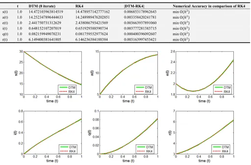
Now, about the efficiency of DTM, we have compared the solution of DTM with the solution of RK4. Matlab codes are used to generate both the solutions. We give the comparison of numerical results for the compartments in table-1. Here we have chosen the time for one month. The profile of

(5)

comparison is performed for a time length of one month. For longer period of time, we give a conjecture that the DTM does not provide a better approximation. Since the epidemic outbreak holds for short interval so we can use DTM to

approximate the solution of an epidemic model. In our opinion, DTM is suitable for solving a system of nonlinear differential equations but efficient for a shorter period of time.

Table 1. The absolute error involved in DTM along with the result obtained by RK4.

t DTM (8 iterate) RK4 |DTM-RK4| Numerical Accuracy in comparison of RK4 s(t) 1.0 14.472103963814519 14.478957142777162 0.006853178962643 min Ο

a(t) 1.0 14.252347896444633 14.248989476202851 0.003358420241781 min Ο

e(t) 1.0 2.441750731312629 2.438086793421569 0.003663937891060 min Ο

i(t) 1.0 0.648152107207019 0.651929388590734 0.003777281383715 min Ο

q(t) 1.0 0.082159949070231 0.081759552977624 0.000400396092607 min Ο

r(t) 1.0 6.149400381641805 6.146236384188384 0.003163997453421 min Ο

Figure 2. Compartments versus time (t) for DTM and RK4. Figure is generated in Matlab.

Although the results found by DTM are satisfactory but we can’t comment about the following things, does the system stable? Is there any globally attractor? In the following sections we are going to discuss about these things.

4. Equilibrium Points and Reproduction

Number

In this section, the existence of virus free equilibrium and endemic equilibrium of system (2) is discussed. The basic reproduction number (R) for the SAEIQRS model is calculated.

Equilibrium points are the points where the variables do not change with time. The equilibrium points of the system (2) are found by setting dS dA dE dI dQ dR ₀

dt = dt = dt =dt = dt = dt = in (2).

We get the system of equations,

2 1

1

1 1 2

2 1

1 2

0 0

0

( ) 0

0

B S SI S R S A A AI SI E E AI E k I I I

I k Q Q I Q R A R

µ

β

α

η

α

µ

φ

β

µ

γ

φ

γ

µ

σ

µ

δ

σ

δ

µ

φ

η

− − − + =

 

 ₋ ₋ ₋ ₌ 

 

 ₋ ₋ ₊ ₌ 

 

 

− + − − =

 

 ₋ ₊ ₋ ₌ 

 

+ − + − =

 

 

(10)

4.1. Virus Free Equilibrium

The virus free equilibrium (VFE) of the system (2) is

0 ( 0, 0, 0, 0, 0, 0)

P = S A R . Where,

0

2

2 2

2

2 2

( )( )

,

( )( )( )

( )

,

( )( )( )

µ η µ φ

µ η µ α µ φ α η φ

α µ η

α φ

+ +

=

+ + + −

+ =

+ + + −

=

+ + + −

B S

B A

(6)

4.2. Basic Reproduction Number

The basic reproduction number is defined as the expected number of secondary cases that would arise from the introduction of a single primary infectious case into a fully susceptible population [23]. To obtain the basic reproduction number (R), we will use the next generation matrix approach. Since the model has three infected classes E, I and Q, so to get the basic reproduction number (R) we take only three equations from the system (2) corresponding to these classes. That is,

1

1 1 2

2 1

(

)

(

)

dE

SI

E

AI

dt

dI

E

k I

I

dt

dQ

I

k Q

Q

dt

β

µ

γ

φ

γ

µ

σ

µ

δ





=

−

+



=

−

+

−







=

−

+

−







(11)

Let X=

(

E, I, Q

)

, then (11) can be written as,

( ) ( )

dX

f X v X

dt = − (12)

Where,

1

1 1 2

2 1

( ) ( )

( ) 0 ( ) ( )

0 ( )

S A I E

f X and v X E k I

I k Q

β φ µ γ

γ µ σ σ

σ µ δ

+ +         =_ _ = −_ + + + + _    ₋ ₊ _{+ +}     

Thus the basic reproduction number (R) is,

0 1 0 1 1 2

( )

( )( )

S A

R

k

γ β φ

µ γ µ σ σ

+ =

+ + + + (13)

4.3. Endemic Equilibrium Point

When the disease is present at the population one has

* ₀

I ≠ . There may be several critical points when I*≠0, which are the endemic equilibrium points (EEP) of the

model. These points will be denoted by,

* * * * * * *

( , , , , , )

e

P = S A E I Q R . Where S*,A*,E*,I*,Q*,R* represent the positive solution of the set of system (10).

Solving the system of equations (10) we get,

* * *

* 3 4 2 1 2 1 1 4 2

* *

4 1 2 1 3 2

( ) ( ) ( )

,

{ ( ) ( ) }

φ η φ σ δ σ

β φ α η φ

+ + + +

=

+ + −

B B B B I B I B I

S

B B I B I B

*

* 3 4 1 4 2

* *

4 1 2 1 3 2

( )

,

{ ( ) ( ) }

α α η σ δ σ

β φ α η φ

+ +

=

+ + −

B B B B I

A

B B I B I B

* * *

* 3 4 1 4 2 2 1 1

* *

4 6 1 2 1 3 2

{ ( ) }{ ( ) }

{( )( ) }

BB B B I B I I

E

B B B I B I B

η σ δσ β φ αφ

β φ αηφ

+ + + + = + + − _, * * 2 4 I Q B σ = , * * *

* 1 2 1 1 4 2 2 4

*

4 1 2 1 3 2

( )( )( )

*

{( )( ) }

B I B I B I BB

R

B B I B I B

β φ σ δσ αφ

β φ αηφ

+ + + +

=

+ + −

While *

I is the positive root of the equation,

* 2 *

( ) 0

a I +b I + =c

Here, a=γ β φ η σ1 1B4 +γ β φ η δ σ1 2 −β φ1B B B B3 4 5 6

1 1 4 1 2 4 2 2 2 1

1 3 4 1 1 3 4 5 6 2 3 4 5 6

η σ γ α φ η σ γ β η δ σ γ β η δ σ γ α φ

γ β φ φ β

= + + +

+ − −

b B B B B

B B B B B B B B B B B B B

1 2 3 4 2 4

( )

c= B B B B −αηφ B R

,

1 2 2 3 4 1

,

5 1 2 1 6

, , ,

µ α µ φ µ η µ δ

µ σ σ µ γ

= + = + = + = + +

= + + + = +

B B B B k

B k B

5. Stability Analysis

In this section, the stability analysis of virus free equilibrium point,P₀ and endemic equilibrium point, *

e

P of the system (2) are studied. Analysis of various types of stability for hopfield neural networks are studied in [28, 29, 30]. Here at first we have stated the necessary theorems for stability analysis. Moreover we have used equation (2) to prove the following theorems for this particular model SAEIQRS.

The necessary theorems for stability analysis are stated below.

Theorem 5.1: when R<1, the virus free equilibrium (VFE)

0

P is locally asymptotically stable. When R>1, the virus free equilibrium (VFE) P is an unstable saddle point. ₀

Theorem 5.2: WhenR≤1, the virus free equilibrium P is ₀ globally asymptotically stable.

Theorem 5.3: whenR>1, the endemic equilibrium *

e

P is locally asymptotically stable.

Now we shall proof these theorems using the system of equations (2) generated from SAEIQRS model.

Proof of theorem 5.1: The Jacobian matrices of the model (2) at P₀is

0

2 1 0

1 0 1 0

2

2 1

2 1 1

0

( ) 0 0 0

0 0 0

0 0 0 0

( )

0 0 0 0

0 0 0 ( ) 0

0 0

S

D A

C S A

J P

C

k

D

µ α β η

α φ

β φ

γ

σ µ δ

φ σ δ

                                − + − − − − + = − − + + − where,

1=µ γ+ , 2 =µ+ 1+σ1+σ2, 1 =µ η+ , 2 =µ φ+ 2

C C k D D

By [20], P0 is locally asymptotically stable if all the

eigenvalues of J P( 0) has negative real part. Again

P

₀is

unstable if at least one of the eigenvalues of J P( 0) has

positive real part.

The characteristic polynomial of J P( ₀) is 2

1 1 2 2 1

2

1 2 0 1 0 1 2

( ) ( )( ){ ( ) ( ) }

{ ( ) ( ) }

λ λ µ δ λ µ λ α λ α αη

λ λ γ β φ

= + + + + + + + + + +

+ + − + +

f k D D D D

(7)

The eigenvalues of J P( 0) are, λ1 = −(µ +k1+δ) , 2

λ = −µ ,

2

1 2 1 2 2 1

3, 4

( ) ( ) 4{ ( ) }

2

D D α D D α D D α αη

λ =− + + ± + + − + +

,

and, 1 2 1 2 2 1 2 0 1 0

5 , 6

( ) ( ) 4{ ( ) }

2

C C C C C C γ βS φA

λ =− + ± + − − +

Here λ1,λ2 and λ3,4 are negative. The real part of λ5 , 6

will be negative if C C1 2−γ β( S0+φ1 0A) 0> or R <1. Thus for

1

R< , the real part of all eigenvalues of J P( 0) are negative

and consequently the virus free equilibrium (DEF) P0 is

locally asymptotically stable. Again one of the real part of

5 ,6

λ will be positive if C C1 2−γ β( S0+φ1 0A )<0 or R>1.

Thus for R >1, at least one of the eigenvalues of J P( 0) has

positive real part and consequently the virus free equilibrium (DEF) P0 is unstable saddle point.

Proof of theorem 5.2:According to [20, 24], Consider the following positive definite Lyapunov function

1 1 1 2

1 1 2

( ) ( ) ( ) ( ){ ( ) } ( ) ( ) ( )( ) { ( ) ( )( )} ( )

( )( ){ 1}

( )( )

( )

L E I

SI E E AI E k I

S I E AI E k I

S A k I

S A

k I

k

γ µ γ

γ β µ γ φ µ γ γ µ σ σ

γ β µ γ γ γφ µ γ γ µ γ µ σ σ

γ β φ µ γ µ σ σ

γ β φ

µ γ µ σ σ _{µ γ µ} _{σ σ}

µ γ = + + ′ ′ ′ ⇒ = + + = − − + + + − + + + = − + + + + − + + + + = + − + + + + + = + + + + − + + + +

= + ( 1 1 2)( 1)

0

k R I

µ+ +σ σ+ −

≤

Furthermore, L′ =0 if and only if I =0 or R=1. Thus,

the largest compact invariant set in

{ ( ,S A E I Q R, , , , ) |L′ =0} is the singleton { }P₀ . When 1

R≤ , the global stability of P0 follows from LaSalle’s

invariance principle [25]. So, P0 is globally asymptotically

stable in Ω. When R≥1, it follows from the fact L′ > 0if 0

I > . This completes the proof.

Proof of theorem 5.3: The Jacobian matrix of the model (2) at * ₍ *_, *_, *_, *_, *_, *₎

e

P = S A E I Q R is

* *

2 1 1

* * * *

*

1 1

1 1 2

2 1

0 0 0

0 0

( )

0 0 0 0

0 0

e

I S

I A

I I A S

J P

k

µ β α β η

α µ φ φ φ

β φ µ γ φ β

γ µ σ σ

σ µ δ

φ σ δ µ η

_{− −} ₋ ₋     _{− − −} ₋     _{− −} ₊  =_ _ − − − −    _{− − −}     _{− −}    * *

2 1 1

1 2 1

* ( )

0

µ β α µ φ φ µ γ µ

σ σ µ δ µ η

= − − − − − − − − − − −

− − − − − − <

e

trace J P I I k

k

1 1 1 1

1 2 1

1 2 2 1 1 2 1 1

2 2 1 1

1

φ µ δ γ φ µ β α µ η ηασ

φ γα β µ β α µ η ηδσ γηβ µ δ

φ φ µ φ φ σ γβ µ φ φ µ δ

µ η β ηδσ µ β α µ φ φ µ δ

µ η µ γ µ

= + + + + + − + + + + − + + + − + + + + + + + + − + + + + + + + + + + + * * * * e * * * * * * * * * * *

d et J ( P ) I ( k ) { A ( I )( ) }

I { S ( I )( ) } I ( k )

{ A ( I ) } I ( I ){( k )

( ) S } ( I )( I )( k )

( ){( )( k 1 2 1

2 1 1 1 2 1

σ σ γ φ β

ηαφ µ δ µ η µ σ σ

+ − +

+ + + + + + + −

* *

) ( A S )}

( k )( )( k )( R )

Now det J P( _e*)>0 if R >1 . Thus for R>1 the eigenvalues of *

( e)

J P has negative real part. So by [26] and [27], the endemic equilibrium P_e* is locally asymptotically stable if R>1.

6. Numerical Eigenvalues and Power

Method

This section comprises of two sets of different parameter values. For each set, we have evaluated the eigenvalues numerically and verified theorem 5.1. Moreover, dominant eigenvalues are determined based on the power method.

Based on [13], we consider the value of the parameters

1 2

1 1 2

0.01, 0.09, 0.45, 0.35, 0.3, 0.65, 0.01, 0.05, 0.035, 0.65, 0.2, 0.3

B

k

β γ σ σ δ

η µ α φ φ 

= = = = = =

= = = = = = (14)

Using parameter (14), we get the reproduction number, R= 0.009306122448980, which is less than one. So by

theorem 5.1, the virus free equilibria is asymptotically stable and all the eigenvalues of Jacobian matrix should has negative real part.

We have the Jacobian matrix using parameter (14) at virus free equilibria

1 0

-0.7000 0 0 -0.0015 0 0.0100 0.6500 -0.3500 0 -0.0061 0 0

0 0 -0.5000 0.0076 0 0

0 0 0.4500 -0.7350 0 0

0 0 0 0.3000 -0.7350 0

0 0.3000 0 0.3500 0.6500 -0.0600

J         =           

The eigenvalues of the matrix

J

₀1 are:

-0.690934769394311, -0.369065230605689,

-0.486251190481589, -0.7350, -0.748748809518410, -0.050, which are all negative. So the criterion of theorem 5.1 holds for the set of parameter (14). Using the power method we find the dominant eigenvalue is, -0.748748809518410.

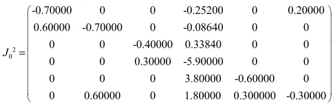
Again based on [14], we consider parameter values

2

1 1 2

0.3, 0.3, 0.3, ₁ 1.8, 3.8, 0.3,

0.2, 0.1, 0.2, 0.6, 0.12, 0.6

B

k

β γ σ σ δ

η µ α φ φ

  

= = = = = =

= = = = = = (15)

(8)

2 0

-0.70000 0 0 -0.25200 0 0.20000

0.60000 -0.70000 0 -0.08640 0 0

0 0 -0.40000 0.33840 0 0

0 0 0.30000 -5.90000 0 0

0 0 0 3.80000 -0.60000 0

0 0.60000 0 1.80000 0.300000 -0.30000

J

 

 

 

=

The eigenvalues corresponds to the matrix 2 0

J

are: -0.8+0.331662479035540i, -0.8-0.331662479035540i, -5.918396647881225, -0.6, -0.381603352118776, -0.1. All of these have negative real part. So the theorem 5.1 holds for the set of parameter (15). And by power method the dominant eigenvalue is, -5.918396647881225.

Thus for both parameter set the reproduction number is less than one and the real parts of the eigenvalues are negative. So the virus free equilibrium (VEF)P₀ is locally asymptotically stable. This verifies theorem 5.1 numerically.

7. Numerical Simulations

In this section, we simulate various compartments of SAEIQRS model. For this, we have used built-in solver ode45 in Matlab. For the set of parameter value in (14), we consider the number of susceptible, antidotal, exposed, infectious, quarantined and recovered computers at the beginning are S(0)=30, A(0)=5, E(0)=3, I(0)=0, Q(0)=0, R(0)=2 respectively. And for the set of parameter value in (15), we consider the number of susceptible, antidotal, exposed, infectious, quarantined and recovered computers at the beginning are S(0)=65, A(0)=20, E(0)=10, I(0)=0, Q(0)=0, R(0)=5 respectively. The behaviors of susceptible, antivirus, exposed, infected, quarantine and recovered class with respect to time for both set of parameter (14) and (15) with their corresponding initial conditions is depicted in figure 3.

Figure 3. Dynamical behavior of the system (2). Figure is generated in Matlab with parameters,B=0 .0 1, β =0 .0 9 , γ =0 .4 5, σ₁=0 .3 5, σ₂=0 .3,

1 1 2 1 2

0 .6 5, 0 .0 1, 0 .0 5, 0 .0 3 5, 0 .6 5, 0 .2, 0 .3, 0 .3, 0 .3, 0 .3, 1 .8, 3 .8, 0 .3,

δ = η = µ = k = α = φ = φ = a n d B= β = γ = σ = σ = δ =

1 1 2

0 . 2 , 0 .1, 0 . 2 , 0 . 6 , 0 .1 2 , 0 . 6

η = µ = k = α = φ = φ = .

Figure 3 is the representative of the behavior of the susceptible, antivirus, exposed, infected, quarantine and recovered class. We get the insight of the behavior of the system regardless of the sets of parameters. As a consequence, we have to choose one set of parameter. Based on the analysis of power method in the previous section we choose the set of parameter, which is in equation (15). Between two sets of parameters this set gives the most dominating eigenvalue. From now, we prefer the values of the parameter in equation (15) for further analysis.

The effect of quarantine class (Q) on infected class (I), quarantine class (Q) on recovered class (R) also infected class (I) on recovered class (R) is depicted in figure 4. We simulate the system with 1000 of different initial conditions. As the simulation runs over time, we observe that different set of initial conditions is approaching to a particular curve. Such behaviors are depicted in figure 4. Point to be noted that

these behavior are not quite visible in this low amplitude. Finally, we conclude that these two figures have global attractor where subsequent iterations converge. Of course, we observe such behavior in the light of numeric.

(9)

immunization user should update their antivirus regularly.

Figure 4. Left panel shows dynamical behavior of quarantine class (Q) on infected class (I), middle panel shows dynamical behavior of quarantine class (Q) on recovered class (R), and right panel shows dynamical behavior of infected class (I) and recovered class (R). Figures are generated in Matlab with parameters,B=0 .3, β=0 .3, γ =0 .3, σ1=1 .8, σ2=3 .8, δ =0 .3,η =0 .2, µ =0 .1, k1=0 .2, α =0 .6 , φ1=0 .1 2, φ2=0 .6.

Figure 5. Effect of recovery rate φ₂ form antidotal (A) compartment on recovered (R) compartment. Other parameters are, B=0 .3, β=0 .3,

1 2 1 1

0.3, 1.8, 3.8, 0.3, 0.2, 0.1, 0.2, 0.6, 0.12.

γ= σ= σ = δ= η= µ= k= α= φ=

8. Conclusion

The model we analyzed is expressed by a system of nonlinear ordinary differential equations. We have developed the SAEIQRS model to understand the transmission of computer viruses. The efficiency and accuracy of the results of DTM are justified based on the results of RK4. We found DTM is convenient to approximate the solution of a system of nonlinear differential for a period of time, which is not lasting long. Virus free equilibrium and endemic equilibrium of the system are analyzed. By the method of next generation matrix, we obtain the basic reproduction number R. The stability of the system as well as the annihilation of the virus depends on the basic reproduction number. Once the basic reproduction number is less than or equal to one, we have shown that the behavior of the model is stable. We also give conjecture that the users can predict virus propagation to some extent. If the reproduction number does not lie in the above-mentioned range, at this point the proposed model will

be unstable and the virus perseveres in the whole population. Numerically, the eigenvalues of Jacobian matrix and the dominant eigenvalue are computed by using two different parameter set. Numerical simulations represent the behavior of different compartments. Based on the analysis, we observed that the dynamics of the system are asymptotically stable. The global stability of virus free equilibrium and the local stability of endemic equilibrium have been proven. Moreover, the whole population in the long term is in a recovery state. Simulation shows, antidotal compartment plays important role in recovery. We have proven mathematically that the user can prevent virus attack by updating their antivirus regularly. Although in real world network it’s very difficult to achieve full immunization by antivirus. To get rid of the virus attack we need a higher recovery rate of

φ

₂. We found a fascinating case where the antidotal compartment plays a crucial role to get our work and data free from virus.

References

[1] J. Aycock. Computer viruses and malware, volume 22. Springer Science & Business Media, 2006.

[2] J. Li and P. Knickerbocker. Functional similarities between computer worms and biological pathogens. Computers & Security, 26(4): 338-347, 2007.

[3] J. O. Kephart, S. R. White, and D. M. Chess. Computers and epidemiology. IEEE Spectrum, 30(5):20-26, 1993.

[4] B. Ebenezer, N. Farai, and A. A. S Kwesi. Fractional dynamics of computer virus propagation. Science Journal of Applied Mathematics and Statistics, 3(3):63-69, 2015. [5] J. Hruska. Computer viruses and anti-virus warfare. Ellis

Horwood, 1992.

[6] E. Al Daoud, I. H. Jebril, and B. Zaqaibeh. Computer virus strategies and detection methods. International Journal of Open Problems Compt. Math, 1(2):12-20, 2008.

(10)

[8] J. O. Kephart and S. R. White. Measuring and modeling computer virus prevalence. In Research in Security and Privacy, Proceedings, IEEE Computer Society Symposium on, pages 2-15. IEEE, 1993.

[9] X. Zhang, S. Chen, H. Lu, and F. Zhang. An improved computer multi-virus propagation model with user awareness. Journal of Information and Computational Science, pages 4301-4308, 2011.

[10] S. Xu, W. Lu, and Z. Zhan. A stochastic model of multivirus dynamics. IEEE Transactions on Dependable and Secure Computing, 9(1):30-45, 2012.

[11] J. R. C. Piqueira, A. A. De Vasconcelos, C. E. C. J. Gabriel, and V. O. Araujo. Dynamic models for computer viruses. Computers & Security, 27(7):355-359, 2008.

[12] B. K. Mishra and A. K. Singh. Two quarantine models on the attack of malicious objects in computer network. Mathematical Problems in Engineering, 2012:1-13, 2011. [13] M. Kumar, B. K. Mishra, and T. C. Panda. Effect of

quarantine and vaccination on infectious nodes in computer network. International Journal of Computer Networks and Applications, 2(2):92-98, 2015.

[14] B. K. Mishra and N. Jha. SEIQRS model for the transmission of malicious objects in computer network. Applied Mathematical Modelling, 34(3):710-715, 2010.

[15] F. Cohen. Computer viruses: theory and experiments. Computers & Security, 6(1):22-35, 1987.

[16] W. H. Murray. The application of epidemiology to computer viruses. Computers & Security, 7(2):139-145, 1988.

[17] W. O. Kermack and A. G. McKendrick. A contribution to the mathematical theory of epidemics. In Proceedings of the Royal Society of London A: mathematical, physical and engineering sciences, volume 115, pages 700-721. The Royal Society, 1927.

[18] W. O. Kermack and A. G. McKendrick. Contributions to the mathematical theory of epidemics II, the problem of endemicity. In Proceedings of the Royal Society of London A: mathematical, physical and engineering sciences, volume 138, pages 55-83. The Royal Society, 1932.

[19] J. O. Kephart and S. R. White. Directed-graph

epidemiological models of computer viruses. In Research in Security and Privacy, 1991. Proceedings, 1991 IEEE Computer Society Symposium on, pages 343-359. IEEE, 1991. [20] F. Wang, Y. Yang, D. Zhao, and Y. Zhang. A worm defending

model with partial immunization and its stability analysis. Journal of Communications, 10(4):276-283, 2015.

[21] I. H. A. H. Hassan. Application to Differential Transformation Method for Solving Systems of Differential Equations. Applied Mathematical Modeling, 32 (2008), PP. 2552–2559. [22] A. K. Chakraborty, P. Shahrear, M. A. Islam, Analysis of

Epidemic Model by Differential Transform Method. Journal of Multidisciplinary Engineering Science and Technology, 4(2): 6574-6581, 2017.

[23] B. K. Mishra and A. Prajapati. Spread of malicious objects in computer network: A fuzzy approach. Applications & Applied Mathematics, 8(2):684-700, 2013.

[24] A. L. V. Barber, C. C. Chavez, and E. Barany. Dynamics of an SAIQR influenza model. BIOMATH, 3(2):1409251, 2014. [25] J. P. LaSalle. The stability of dynamical systems, volume 25.

SIAM, 1976.

[26] F. Brauer and C. C. Chavez. Mathematical models in population biology and epidemiology, volume 40. Springer, 2001.

[27] M. A. Khan, Z. Ali, L. C. C. Dennis, I. Khan, S. Islam, M. Ullah, and T. Gul. Stability analysis of an SVIR epidemic model with non-linear saturated incidence rate. Applied Mathematical Sciences, 9(23):1145-1158, 2015.

[28] A. Arbi, C. Aouiti, F. Chérif, A. Touati and A. M. Alimi. Stability analysis for delayed high-order type of Hopfield neural networks with impulses. Neurocomputing, volume 165, pages 312-329, 2015

[29] A. Arbi, C. Aouiti, F. Chérif, A. Touati and A. M. Alimi. Stability analysis of delayed Hopfield neural networks with impulses via inequality techniques. Neurocomputing, volume 158, pages 281-294, 2015.