Union Support Recovery in Multi-task Learning
Mladen Kolar [email protected]
John Lafferty [email protected]
Larry Wasserman [email protected]
School of Computer Science Carnegie Mellon University 5000 Forbes Avenue Pittsburgh, PA 15213, USA
Editor: Hui Zou
Abstract
We sharply characterize the performance of different penalization schemes for the problem of se-lecting the relevant variables in the multi-task setting. Previous work focuses on the regression problem where conditions on the design matrix complicate the analysis. A clearer and simpler pic-ture emerges by studying the Normal means model. This model, often used in the field of statistics, is a simplified model that provides a laboratory for studying complex procedures.
Keywords: high-dimensional inference, multi-task learning, sparsity, normal means, minimax estimation
1. Introduction
We consider the problem of estimating a sparse signal in the presence of noise. It has been em-pirically observed, on various data sets ranging from cognitive neuroscience (Liu et al., 2009) to genome-wide association mapping studies (Kim et al., 2009), that considering related estimation tasks jointly can improve estimation performance. Because of this, joint estimation from related tasks or multi-task learning has received much attention in the machine learning and statistics com-munity (see for example Turlach et al., 2005; Zou and Yuan, 2008; Zhang, 2006; Negahban and Wainwright, 2009; Obozinski et al., 2011; Lounici et al., 2009; Liu et al., 2009; Lounici et al., 2010; Argyriou et al., 2008; Kim et al., 2009, and references therein). However, the theory behind multi-task learning is not yet settled.
An example of multi-task learning is the problem of estimating the coefficients of several mul-tiple regressions
yj=Xjβj+ǫj, j∈[k] (1)
where Xj∈Rn×p is the design matrix, yj ∈Rnis the vector of observations, ǫj∈Rn is the noise vector andβj ∈Rp is the unknown vector of regression coefficients for the j-th task, with[k] =
{1, . . . ,k}.
When the number of variables p is much larger than the sample size n, it is commonly assumed that the regression coefficients are jointly sparse, that is, there exists a small subset S⊂[p]of the regression coefficients, with s :=|S| ≪n, that are non-zero for all or most of the tasks.
Kolar and Xing (2010). Obozinski et al. (2011) propose to minimize the penalized least squares objective with a mixed (2,1)-norm on the coefficients as the penalty term. The authors focus on consistent estimation of the support set S, albeit under the assumption that the number of tasks k is fixed. Negahban and Wainwright (2009) use the mixed(∞,1)-norm to penalize the coefficients and focus on the exact recovery of the non-zero pattern of the regression coefficients, rather than the support set S. For a rather limited case of k=2, the authors show that when the regression do not share a common support, it may be harmful to consider the regression problems jointly using the mixed(∞,1)-norm penalty. Kolar and Xing (2010) address the feature selection properties of simultaneous greedy forward selection. However, it is not clear what the benefits are compared to the ordinary forward selection done on each task separately. In Lounici et al. (2009) and Lounici et al. (2010), the focus is shifted from the consistent selection to benefits of the joint estimation for the prediction accuracy and consistent estimation. The number of tasks k is allowed to increase with the sample size. However, it is assumed that all tasks share the same features; that is, a relevant coefficient is non-zero for all tasks.
Despite these previous investigations, the theory is far from settled. A simple clear picture of when sharing between tasks actually improves performance has not emerged. In particular, to the best of our knowledge, there has been no previous work that sharply characterizes the performance of different penalization schemes on the problem of selecting the relevant variables in the multi-task setting.
In this paper we study multi-task learning in the context of the many Normal means model. This is a simplified model that is often useful for studying the theoretical properties of statistical procedures. The use of the many Normal means model is fairly common in statistics but appears to be less common in machine learning. Our results provide a sharp characterization of the sparsity patterns under which the Lasso procedure performs better than the group Lasso. Similarly, our results characterize how the group Lasso (with the mixed (2,1) norm) can perform better when each non-zero row is dense.
1.1 The Normal Means Model
The simplest Normal means model has the form
Yi=µi+σεi, i=1, . . . ,p (2)
where µ1, . . . ,µp are unknown parameters and ε1, . . . ,εp are independent, identically distributed Normal random variables with mean 0 and variance 1. There are a variety of results (Brown and Low, 1996; Nussbaum, 1996) showing that many learning problems can be converted into a Nor-mal means problem. This implies that results obtained in the NorNor-mal means setting can be trans-ferred to many other settings. As a simple example, consider the nonparametric regression model
Zi =m(i/n) +δi where m is a smooth function on [0,1]and δi ∼N(0,1). Let φ1,φ2, . . . , be an orthonormal basis on [0,1] and write m(x) =∑∞j=1µjφj(x)where µj=
R1
0m(x)φj(x)dx. To estimate the regression function m we need only estimate µ1,µ2, . . . ,. Let Yj =n−1∑ni=1Ziφj(i/n). Then
However, the most important aspect of the Normal means model is that it allows a clean setting for studying complex problems. In this paper, we consider the following Normal means model. Let
Yi j∼
(1−ε)
N
(0,σ2) +εN
(µi j,σ2) j∈[k], i∈S
N(0,σ2) j∈[k], i∈Sc (3)
where(µi j)i,jare unknown real numbers,σ=σ0/√n is the variance withσ0>0 known,(Yi j)i,jare random observations,ε∈[0,1]is the parameter that controls the sparsity of features across tasks and S⊂[p]is the set of relevant features. Let s=|S|denote the number of relevant features. Denote the matrix M∈Rp×k of means
Tasks
1 2 . . . k
1 µ11 µ12 . . . µ1k 2 µ21 µ22 . . . µ2k
..
. ... ... . .. ...
p µp1 µp2 . . . µpk
and letθi= (µi j)j∈[k]denote the i-th row of the matrix M. The set Sc= [p]\S indexes the zero rows
of the matrix M and the associated observations are distributed according to the Normal distribu-tion with zero mean and varianceσ2. The rows indexed by S are non-zero and the corresponding observation are coming from a mixture of two Normal distributions. The parameterεdetermines the proportion of observations coming from a Normal distribution with non-zero mean. The reader should regard each column as one vector of parameters that we want to estimate. The question is whether sharing across columns improves the estimation performance.
It is known from the work on the Lasso that in regression problems, the design matrix needs to satisfy certain conditions in order for the Lasso to correctly identify the support S (see van de Geer and B¨uhlmann, 2009, for an extensive discussion on the different conditions). These regularity con-ditions are essentially unavoidable. However, the Normal means model (3) allows us to analyze the estimation procedure in (4) and focus on the scaling of the important parameters(n,k,p,s,ε,µmin) for the success of the support recovery. Using the model (3) and the estimation procedure in (4), we are able to identify regimes in which estimating the support is more efficient using the ordinary Lasso than with the multi-task Lasso and vice versa. Our results suggest that the multi-task Lasso does not outperform the ordinary Lasso when the features are not considerably shared across tasks; thus, practitioners should be careful when applying the multi-task Lasso without knowledge of the task structure.
An alternative representation of the model is
Yi j=
N
(ξi jµi j,σ2) j∈[k], i∈SN(0,σ2) j∈[k], i∈Sc
where ξi j is a Bernoulli random variable with success probability ε. Throughout the paper, we will set ε=k−β for some parameterβ∈[0,1);β<1/2 corresponds to dense rows andβ>1/2 corresponds to sparse rows. Let µmindenote the following quantity µmin=min|µi j|.
Under the model (3), we analyze penalized least squares procedures of the form
b
µ=argmin
µ∈Rp×k
1
2||Y−µ|| 2
where||A||F =∑jkA2jkis the Frobenious norm, pen(·)is a penalty function andµis a p×k matrix of means. We consider the following penalties:
1. theℓ1penalty
pen(µ) =λ
∑
i∈[p]j
∑
∈[k] |µi j|,which corresponds to the Lasso procedure applied on each task independently, and denote the resulting estimate asµbℓ1
2. the mixed(2,1)-norm penalty
pen(µ) =λ
∑
i∈[p] ||θi||2,
which corresponds to the multi-task Lasso formulation in Obozinski et al. (2011) and Lounici et al. (2009), and denote the resulting estimate asµbℓ1/ℓ2
3. the mixed(∞,1)-norm penalty
pen(µ) =λ
∑
i∈[p] ||θi||∞,
which correspond to the multi-task Lasso formulation in Negahban and Wainwright (2009), and denote the resulting estimate asµbℓ1/ℓ∞.
For any solutionµbof (4), let S(µb)denote the set of estimated non-zero rows
S(µb) ={i∈[p] : ||θbi||26=0}.
We establish sufficient conditions under whichP[S(µb)6=S]≤αfor different methods. These results are complemented with necessary conditions for the recovery of the support set S.
In this paper, we focus our attention on the three penalties outlined above. There is a large literature on the penalized least squares estimation using concave penalties as introduced in Fan and Li (2001). These penalization methods have better theoretical properties in the presence of the design matrix, especially when the design matrix is far from satisfying the irrepresentable condition (Zhao and Yu, 2006). In the Normal means model, due to the lack of the design matrix, there is no advantage to concave penalties in terms of variable selection.
1.2 Overview of the Main Results
The main contributions of the paper can be summarized as follows.
1. We establish a lower bound on the parameter µminas a function of the parameters(n,k,p,s,β). Our result can be interpreted as follows: for any estimation procedure there exists a model given by (3) with non-zero elements equal to µmin such that the estimation procedure will make an error when identifying the set S with probability bounded away from zero.
By comparing the lower bounds with the sufficient conditions, we are able to identify regimes in which each procedure is optimal for the problem of identifying the set of non-zero rows S. Fur-thermore, we point out that the usage of the popular group Lasso with the mixed(∞,1)norm can be disastrous when features are not perfectly shared among tasks. This is further demonstrated through an empirical study.
1.3 Organization of the Paper
The paper is organized as follows. We start by analyzing the lower bound for any procedure for the problem of identifying the set of non-zero rows in Section 2. In Section 3 we provide sufficient conditions on the signal strength µminfor the Lasso and the group Lasso to be able to detect the set of non-zero rows S. In the following section, we propose an improved approach to the problem of estimating the set S. Results of a small empirical study are reported in Section 4. We close the paper by a discussion of our findings.
2. Lower Bound on the Support Recovery
In this section, we derive a lower bound for the problem of identifying the correct variables. In particular, we derive conditions on(n,k,p,s,ε,µmin)under which any method is going to make an error when estimating the correct variables. Intuitively, if µmin is very small, a non-zero row may be hard to distinguish from a zero row. Similarly, ifεis very small, many elements in a row will be zero and, again, as a result it may be difficult to identify a non-zero row. Before, we give the main result of the section, we introduce the class of models that are going to be considered.
Let
F
[µ]:={θ∈Rk : minj |θj| ≥µ}
denote the set of feasible non-zero rows. For each j∈ {0,1, . . . ,k}, let
M
(j,k)be the class of all the subsets of{1, . . . ,k}of cardinality j. LetM[µ,s] = [
ω∈M(s,p)
n
(θ1, . . . ,θp)′∈Rp×k : θi∈
F
[µ]if i∈ω, θi=0 if i6∈ω o(5)
be the class of all feasible matrix means. For a matrix M∈M[µ,s], letPM denote the joint law of
{Yi j}i∈[p],j∈[k]. SincePMis a product measure, we can writePM=⊗i∈[p]Pθi. For a non-zero rowθi,
we set
Pθi(A) =
Z
N
(A;θb,σ2Ik)dν(θb), A∈B
(Rk),where ν is the distribution of the random variable ∑j∈[k]µi jξjej with ξj ∼Bernoulli(k−β) and
{ej}j∈[k]denoting the canonical basis ofRk. For a zero rowθi=0, we set
P0(A) =
N
(A; 0,σ2Ik), A∈
B
(Rk).With this notation, we have the following result.
Theorem 1 Let
where
u=
ln1+α2(p−2s+1)
2k1−2β .
Ifα∈(0,1
2)and k−βu<1, then for all µ≤µmin, inf
bµ M∈supM[µ,s]PM[S(bµ)6=S(M)]≥ 1 2(1−α)
whereM[µ,s]is given by (5).
The result can be interpreted in words in the following way: whatever the estimation procedure b
µ, there exists some matrix M∈M[µmin,s]such that the probability of incorrectly identifying the support S(M) is bounded away from zero. In the next section, we will see that some estimation procedures achieve the lower bound given in Theorem 1.
3. Upper Bounds on the Support Recovery
In this section, we present sufficient conditions on(n,p,k,ε,µmin) for different estimation proce-dures, so that
P[S(µb)6=S]≤α.
Letα′,δ′>0 be two parameters such thatα′+δ′=α. The parameterα′controls the probability of making a type one error
P[∃i∈[p] : i∈S(µb)and i6∈S]≤α′,
that is, the parameterα′ upper bounds the probability that there is a zero row of the matrix M that is estimated as a non-zero row. Likewise, the parameterδ′controls the probability of making a type two error
P[∃i∈[p] : i6∈S(µb)and i∈S]≤δ′,
that is, the parameterδ′ upper bounds the probability that there is a non-zero row of the matrix M that is estimated as a zero row.
The control of the type one and type two errors is established through the tuning parameterλ. It can be seen that if the parameterλis chosen such that, for all i∈S, it holds thatP[i6∈S(µb)]≤δ′/s
and, for all i∈Sc, it hold thatP[i∈S(µb)]≤α′/(p−s), then using the union bound we have that P[S(µb)6=S]≤α. In the following subsections, we will use the outlined strategy to chooseλfor different estimation procedures.
3.1 Upper Bounds for the Lasso
Recall that the Lasso estimator is given as
b
µℓ1 =argmin
µ∈Rp×k
1
2||Y−µ|| 2
F+λ||µ||1.
It is easy to see that the solution of the above estimation problem is given as the following soft-thresholding operation
b
µℓ1
i j =
1− λ
|Yi j|
+
where(x)+:=max(0,x). From (6), it is obvious that i∈S(µbℓ1)if and only if the maximum statistic,
defined as
Mk(i) =max j |Yi j|,
satisfies Mk(i)≥λ. Therefore it is crucial to find the critical value of the parameterλsuch that
P[Mk(i)<λ] < δ′/s i∈S P[Mk(i)≥λ] < α′/(p−s) i∈Sc.
We start by controlling the type one error. For i∈Scit holds that
P[Mk(i)≥λ]≤kP[|
N
(0,σ2)| ≥λ]≤ 2kσ√2πλexp − λ 2 2σ2
(7)
using a standard tail bound for the Normal distribution. Setting the right hand side toα′/(p−s)in the above display, we obtain thatλcan be set as
λ=σ
s
2 ln2k√(p−s)
2πα′ (8)
and (7) holds as soon as 2 ln2k√(p−s)
2πα′ ≥1. Next, we deal with the type two error. Let
πk=P[|(1−ε)
N
(0,σ2) +εN
(µmin,σ2)|>λ]. (9) Then for i∈S, P[Mk(i)<λ]≤P[Bin(k,πk) =0], where Bin(k,πk) denotes the binomial random variable with parameters(k,πk). Control of the type two error is going to be established through careful analysis ofπkfor various regimes of problem parameters.Theorem 2 Letλbe defined by (8). Suppose µminsatisfies one of the following two cases:
(i) µmin=σ
√
2r ln k where
r>p1+Ck,p,s− p
1−β 2
with
Ck,p,s=
ln2√(p−s) 2πα′ ln k
and limn→∞Ck,p,s∈[0,∞);
(ii) µmin≥λwhen
lim n→∞
ln k ln(p−s)=0
and k1−β/2≥ln(s/δ′). Then
The proof is given in Section 6.2. The two different cases describe two different regimes character-ized by the ratio of ln k and ln(p−s).
Now we can compare the lower bound on µ2
min from Theorem 1 and the upper bound from
Theorem 2. Without loss of generality we assume thatσ=1. We have that whenβ<1/2 the lower bound is of the order
O
ln kβ−1/2ln(p−s) and the upper bound is of the order ln(k(p−s)). Ignoring the logarithmic terms in p and s, we have that the lower bound is of the orderO
e(kβ−1/2)and the upper bound is of the order
O
e(ln k), which implies that the Lasso does not achieve the lower bound when the non-zero rows are dense. When the non-zero rows are sparse, β>1/2, we have that both the lower and upper bound are of the orderO
e(ln k)(ignoring the terms depending on p ands).
3.2 Upper Bounds for the Group Lasso
Recall that the group Lasso estimator is given as
b
µℓ1/ℓ2 =argmin
µ∈Rp×k
1
2||Y−µ|| 2
F+λ
∑
i∈[p]||θi||2,
whereθi= (µi j)j∈[k]. The group Lasso estimator can be obtained in a closed form as a result of the
following thresholding operation (see, for example, Friedman et al., 2010)
b θℓ1/ℓ2
i =
1− λ
||Yi·||2
+
Yi· (10)
where Yi· is the ith row of the data. From (10), it is obvious that i∈S(µbℓ1/ℓ2) if and only if the
statistic defined as
Sk(i) =
∑
jYi j2,
satisfies Sk(i)≥λ. The choice ofλis crucial for the control of type one and type two errors. We use the following result, which directly follows from Theorem 2 in Baraud (2002).
Lemma 3 Let{Yi= fi+σξi}i∈[n] be a sequence of independent observations, where f ={fi}i∈[n]
is a sequence of numbers,ξiiid∼
N
(0,1)andσis a known positive constant. Suppose that tn,α∈R satisfiesP[χ2n>tn,α]≤α. Let
φα=I{
∑
i∈[n]
Yi2≥tn,ασ2} be a test for f =0 versus f 6=0. Then the testφαsatisfies
P[φα=1]≤α
when f =0 and
P[φα=0]≤δ
for all f such that
||f||2 2≥2(
√
5+4)σ2ln
2e αδ
Proof This follows immediately from Theorem 2 in Baraud (2002).
It follows directly from lemma 3 that setting
λ=tn,α′/(p−s)σ2 (11) will control the probability of type one error at the desired level, that is,
P[Sk(i)≥λ]≤α′/(p−s), ∀i∈Sc.
The following theorem gives us the control of the type two error.
Theorem 4 Letλ=tn,α′/(p−s)σ2. Then
P[S(µbℓ1/ℓ2)6=S]≤α
if
µmin≥σ q
2(√5+4)
s
k−1/2+β
1−c
r
ln2e(2s−δ′)(p−s) α′δ′
where c=p2 ln(2s/δ′)/k1−β. The proof is given in Section 6.3.
Using Theorem 1 and Theorem 4 we can compare the lower bound on µ2
min and the upper bound. Without loss of generality we assume thatσ=1. When each non-zero row is dense, that is, whenβ<1/2, we have that both lower and upper bounds are of the order
O
e(kβ−1/2)(ignoring the logarithmic terms in p and s). This suggest that the group Lasso performs better than the Lasso for the case where there is a lot of feature sharing between different tasks. Recall from previous section that the Lasso in this setting does not have the optimal dependence on k. However, whenβ>1/2, that is, in the sparse non-zero row regime, we see that the lower bound is of the orderO
e(ln(k))whereas the upper bound is of the order
O
e(kβ−1/2). This implies that the group Lasso does not have optimal dependence on k in the sparse non-zero row setting.3.3 Upper Bounds for the Group Lasso with the Mixed(∞,1)Norm
In this section, we analyze the group Lasso estimator with the mixed(∞,1)norm, defined as
b
µℓ1/ℓ∞=argmin
µ∈Rp×k
1
2||Y−µ|| 2
F+λ
∑
i∈[p]||θi||∞,
whereθi = (µi j)j∈[k]. The closed form solution forµbℓ1/ℓ∞ can be obtained (see Liu et al., 2009),
however, we are only going to use the following lemma.
Lemma 5 (Liu et al., 2009)θbℓ1/ℓ∞
i =0 if and only if∑j|Yi j| ≤λ.
Proof See the proof of Proposition 5 in Liu et al. (2009).
Suppose that the penalty parameterλis set as
λ=kσ
r
2 lnk(p−s)
It follows immediately using a tail bound for the Normal distribution that
P[
∑
j
|Yi j| ≥λ]≤k max j
P[|Yi j| ≥λ/k]≤α′/(p−s), ∀i∈Sc,
which implies that the probability of the type one error is controlled at the desired level.
Theorem 6 Let the penalty parameterλbe defined by (12). Then
P[S(µbℓ1/ℓ∞)6=S]≤α
if
µmin ≥ 1+τ
1−ck
−1+βλ
where c=p2 ln(2s/δ′)/k1−βandτ=σq2k ln2s−δ′
δ′ /λ.
The proof is given in Section 6.4.
Comparing upper bounds for the Lasso and the group Lasso with the mixed (2,1)norm with the result of Theorem 6, we can see that both the Lasso and the group Lasso have better dependence on k than the group Lasso with the mixed(∞,1)norm. The difference becomes more pronounced asβincreases. This suggest that we should be very cautious when using the group Lasso with the mixed(∞,1)norm, since as soon as the tasks do not share exactly the same features, the other two procedures have much better performance on identifying the set of non-zero rows.
4. Simulation Results
We conduct a small-scale empirical study of the performance of the Lasso and the group Lasso (both with the mixed(2,1)norm and with the mixed (∞,1) norm). Our empirical study shows that the theoretical findings of Section 3 describe sharply the behavior of procedures even for small sample studies. In particular, we demonstrate that as the minimum signal level µminvaries in the model (3), our theory sharply determines points at which probability of identifying non-zero rows of matrix M successfully transitions from 0 to 1 for different procedures.
The simulation procedure can be described as follows. Without loss of generality we let S= [s]
and draw the samples{Yi j}i∈[p],j∈[k] according to the model in (3). The total number of rows p is
varied in{128,256,512,1024}and the number of columns is set to k=⌊p log2(p)⌋. The sparsity of each non-zero row is controlled by changing the parameterβin{0,0.25,0.5,0.75}and setting ε=k−β. The number of non-zero rows is set to s=⌊log2(p)⌋, the sample size is set to n=0.1p andσ0=1. The parametersα′ andδ′ are both set to 0.01. For each setting of the parameters, we report our results averaged over 1000 simulation runs. Simulations with other choices of parameters
n,s and k have been tried out, but the results were qualitatively similar and, hence, we do not report
them here.
4.1 Lasso
We investigate the performance on the Lasso for the purpose of estimating the set of non-zero rows,
S. Figure 1 plots the probability of success as a function of the signal strength. On the same figure
we plot the probability of success for the group Lasso with both (2,1) and(∞,1)-mixed norms. Using theorem 2, we set
µlasso= p
2(r+0.001)ln k (13)
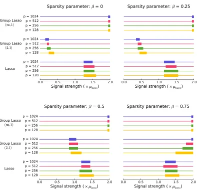
where r is defined in theorem 2. Next, we generate data according to (3) with all elements{µi j} set to µ=ρµlasso, whereρ∈[0.05,2]. The penalty parameterλis chosen as in (8). Figure 1 plots probability of success as a function of the parameterρ, which controls the signal strength. This probability transitions very sharply from 0 to 1. A rectangle on a horizontal line represents points at which the probabilityP[Sb=S]is between 0.05 and 0.95. From each subfigure in Figure 1, we can observe that the probability of success for the Lasso transitions from 0 to 1 for the same value of the parameterρfor different values of p, which indicates that, except for constants, our theory correctly characterizes the scaling of µmin. In addition, we can see that the Lasso outperforms the group Lasso (with(2,1)-mixed norm) when each non-zero row is very sparse (the parameterβis close to one).
4.2 Group Lasso
Next, we focus on the empirical performance of the group Lasso with the mixed(2,1)norm. Fig-ure 2 plots the probability of success as a function of the signal strength. Using theorem 4, we set
µgroup=σ q
2(√5+4)
s
k−1/2+β
1−c
r
ln(2s−δ′)(p−s)
α′δ′ (14)
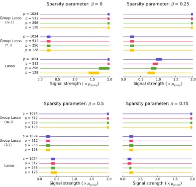
where c is defined in theorem 4. Next, we generate data according to (3) with all elements{µi j}set to µ=ρµgroup, whereρ∈[0.05,2]. The penalty parameterλis given by (11). Figure 2 plots prob-ability of success as a function of the parameterρ, which controls the signal strength. A rectangle on a horizontal line represents points at which the probabilityP[Sb=S]is between 0.05 and 0.95. From each subfigure in Figure 2, we can observe that the probability of success for the group Lasso transitions from 0 to 1 for the same value of the parameterρfor different values of p, which indi-cated that, except for constants, our theory correctly characterizes the scaling of µmin. We observe also that the group Lasso outperforms the Lasso when each non-zero row is not too sparse, that is, when there is a considerable overlap of features between different tasks.
4.3 Group Lasso with the Mixed(∞,1)Norm
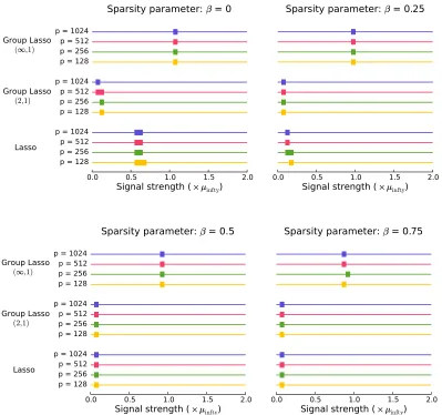
Next, we focus on the empirical performance of the group Lasso with the mixed(∞,1)norm. Fig-ure 3 plots the probability of success as a function of the signal strength. Using theorem 6, we set
µinfty= 1+τ
1−ck
−1+βλ (15)
Probability of successful support recovery: Lasso
0.0 0.5 1.0 1.5 2.0
Signal strength (
lasso)
p = 128p = 256 p = 512 p = 1024 p = 128 p = 256 p = 512 p = 1024 p = 128 p = 256 p = 512 p = 1024
Lasso Group Lasso Group Lasso
(2,1) (,1)
Sparsity parameter:
= 0
0.0 0.5 1.0 1.5 2.0
Signal strength (
lasso)
Sparsity parameter:
= 0.25
0.0 0.5 1.0 1.5 2.0
Signal strength (
lasso)
p = 128p = 256 p = 512 p = 1024 p = 128 p = 256 p = 512 p = 1024 p = 128 p = 256 p = 512 p = 1024
Lasso Group Lasso Group Lasso
(2,1) ( ,1)
Sparsity parameter:
= 0.5
0.0 0.5 1.0 1.5 2.0
Signal strength (
lasso)
Sparsity parameter:
= 0.75
Figure 1: The probability of success for the Lasso for the problem of estimating S plotted against the signal strength, which is varied as a multiple of µlassodefined in (13). A rectangle on each horizontal line represents points at which the probabilityP[Sb=S]is between 0.05 and 0.95. To the left of the rectangle the probability is smaller than 0.05, while to the right the probability is larger than 0.95. Different subplots represent the probability of success as the sparsity parameterβchanges.
in Figure 3, we can observe that the probability of success for the group Lasso transitions from 0 to 1 for the same value of the parameter ρfor different values of p, which indicated that, except for constants, our theory correctly characterizes the scaling of µmin. We also observe that the group Lasso with the mixed(∞,1)norm never outperforms the Lasso or the group Lasso with the mixed
Probability of successful support recovery: group Lasso
0.0 0.5 1.0 1.5 2.0
Signal strength (
group)
p = 128p = 256 p = 512 p = 1024 p = 128 p = 256 p = 512 p = 1024 p = 128 p = 256 p = 512 p = 1024
Lasso Group Lasso Group Lasso
(2,1) (,1)
Sparsity parameter:
= 0
0.0 0.5 1.0 1.5 2.0
Signal strength (
group)
Sparsity parameter:
= 0.25
0.0 0.5 1.0 1.5 2.0
Signal strength (
group)
p = 128p = 256 p = 512 p = 1024 p = 128 p = 256 p = 512 p = 1024 p = 128 p = 256 p = 512 p = 1024
Lasso Group Lasso Group Lasso
(2,1) (,1)
Sparsity parameter:
= 0.5
0.0 0.5 1.0 1.5 2.0
Signal strength (
group)
Sparsity parameter:
= 0.75
Figure 2: The probability of success for the group Lasso for the problem of estimating S plotted against the signal strength, which is varied as a multiple of µgroup defined in (14). A rectangle on each horizontal line represents points at which the probability P[Sb=S]is between 0.05 and 0.95. To the left of the rectangle the probability is smaller than 0.05, while to the right the probability is larger than 0.95. Different subplots represent the probability of success as the sparsity parameterβchanges.
5. Discussion
Probability of successful support recovery: group Lasso with the mixed(∞,1)norm
0.0 0.5 1.0 1.5 2.0
Signal strength (
infty)
p = 128p = 256 p = 512 p = 1024 p = 128 p = 256 p = 512 p = 1024 p = 128 p = 256 p = 512 p = 1024
Lasso Group Lasso Group Lasso
(2,1) (,1)
Sparsity parameter:
= 0
0.0 0.5 1.0 1.5 2.0
Signal strength (
!infty)
Sparsity parameter:
"= 0.25
0.0 0.5 1.0 1.5 2.0
Signal strength (
#$infty)
p = 128p = 256 p = 512 p = 1024 p = 128 p = 256 p = 512 p = 1024 p = 128 p = 256 p = 512 p = 1024
Lasso Group Lasso Group Lasso
(2,1) (%,1)
Sparsity parameter:
&= 0.5
0.0 0.5 1.0 1.5 2.0
Signal strength (
'(infty)
Sparsity parameter:
)= 0.75
Figure 3: The probability of success for the group Lasso with mixed(∞,1)norm for the problem of estimating S plotted against the signal strength, which is varied as a multiple of µinfty defined in (15). A rectangle on each horizontal line represents points at which the prob-abilityP[Sb=S]is between 0.05 and 0.95. To the left of the rectangle the probability is smaller than 0.05, while to the right the probability is larger than 0.95. Different subplots represent the probability of success as the sparsity parameterβchanges.
performs better when each non-zero row is dense. Since in many practical situations one does not know how much overlap there is between different tasks, it would be useful to combine the Lasso and the group Lasso in order to improve the performance. For example, one can take the union of the Lasso and the group Lasso estimate, Sb=S(µbℓ1)∪S(µbℓ1/ℓ2). The suggested approach has the
The analysis of the Normal means model in (3) provides insights into the theoretical results we could expect in the conventional multi-task learning given in (1). However, there is no direct way to translate our results into valid results for the model in (1); a separate analysis needs to be done in order to establish sharp theoretical results.
6. Proofs
This section collects technical proofs of the results presented in the paper. Throughout the section we use c1,c2, . . .to denote positive constants whose value may change from line to line.
6.1 Proof of Theorem 1
Without loss of generality, we may assumeσ=1. Let φ(u)be the density of
N
(0,1)and define P0 andP1 to be two probability measures onRk with the densities with respect to the Lebesgue measure given asf0(a1, . . . ,ak) =
∏
j∈[k]φ(aj) (16)
and
f1(a1, . . . ,ak) =EZEmEξ
∏
j∈mφ(aj−ξjµmin)
∏
j6∈mφ(aj) (17)
where Z∼Bin(k,k−β), m is a random variable uniformly distributed over
M
(Z,k) and{ξj}j∈[k]is a sequence of Rademacher random variables, independent of Z and m. A Rademacher random variable takes values±1 with probability 12.
To simplify the discussion, suppose that p−s+1 is divisible by 2. Let T = (p−s+1)/2. Using P0andP1, we construct the following three measures,
e
Q=Ps1−1⊗P0p−s+1,
Q0= 1
T j∈{
∑
s,...,p}j odd
Ps1−1⊗P0j−s⊗P1⊗P0p−j
and
Q1= 1
T j∈{
∑
s,...,p}j even
Ps1−1⊗P0j−s⊗P1⊗P0p−j.
It holds that
inf
bµ Msup∈MPM[S(M)6=S(bµ)]≥infΨ max
Q0(Ψ=1),Q1(Ψ=0)
≥12−12||Q0−Q1||1,
Q0andQ1. Let g=dP1/dP0and let ui∈Rkfor each i∈[p], then
dQ0
dQe (u1, . . . ,up)
= 1
T j∈{
∑
s,...,p}j even
∏
i∈{1,...,s−1}
dP1
dP1(ui)
∏
i∈{s,...,j−1}dP0
dP0(ui)
dP1
dP0(uj)
∏
i∈{j+1,...,p}dP0
dP0(ui)
= 1
T j∈{
∑
s,...,p}j even
g(uj)
and, similarly, we can compute dQ1/dQe. The following holds
kQ0−Q1k21
=
Z
T1
∑
j∈{s,...,p}
j even
g(uj)−
∑
j∈{s,...,p}
j odd
g(uj)
∏
i∈{s,...,p}dP0(ui) !2
≤T12
Z
∑
j∈{s,...,p}j even
g(uj)−
∑
j∈{s,...,p}
j odd
g(uj) 2
∏
i∈{s,...,p}
dP0(ui)
= 2
T P0(g
2)
−1,
(18)
where the last equality follows by observing that
Z
∑
j∈{s,...,p}j even
∑
j′∈{s,...,p}j′even
g(uj)g(uj′)
∏
i∈{s,...,p}
i even
dP0(ui) =T P0(g2) +T2−T
and
Z
∑
j∈{s,...,p}j even
∑
j′∈{s,...,p}j′odd
g(uj)g(uj′)
∏
i∈{s,...,p}dP0(ui) =T2.
Next, we proceed to upper boundP0(g2), using some ideas presented in the proof of Theorem 1 in Baraud (2002). Recall definitions of f0and f1in (16) and (17) respectively. Then g=dP1/dP0=
f1/f0and we have
g(a1, . . . ,ak) =EZEmEξ
exp−Zµ
2 min
2 +µminj
∑
∈mξjaj=EZ
exp−Zµ
2 min 2
Emh
∏
j∈mcosh(µminaj) i
Furthermore, let Z′∼Bin(k,k−β)be independent of Z and m′uniformly distributed over
M
(Z′,k). The following holdsP0(g2) =P0
EZ′,Z h
exp−(Z+Z ′)µ2
min 2
Em,m′
∏
j∈mcosh(µminaj)
∏
j∈m′cosh(µminaj) i
=EZ′,Z h
exp−(Z+Z ′)µ2
min 2
Em,m′ h
∏
j∈m∩m′ Z
cosh2(µminaj)φ(aj)daj
∏
j∈m△m′ Z
cosh(µminaj)φ(aj)daj ii
,
where we use m△m′to denote(m∪m′)\(m∩m′). By direct calculation, we have that Z
cosh2(µminaj)φ(aj)daj=exp(µ2min)cosh(µ2min)
and Z
cosh(µminaj)φ(aj)daj=exp(µ2min/2). Since 12|m△m′|+|m∩m′|= (Z+Z′)/2, we have that
P0(g2) =EZ,Z′ h
Em,m′ h
cosh(µ2min)|m∩m′|ii =EZ,Z′
h k
∑
j=0
pj cosh(µ2min) ji
=EZ,Z′ h
EXhcosh(µ2min)Xii, where
pj=
0 if j<Z+Z′−k or j>min(Z,Z′) (Z′
j)( k−Z′
Z−j)
(k Z)
otherwise
and P[X = j] =pj. Therefore, X follows a hypergeometric distribution with parameters k, Z, Z′/k. [The first parameter denotes the total number of stones in an urn, the second parameter denotes the number of stones we are going to sample without replacement from the urn and the last parameter denotes the fraction of white stones in the urn.] Then following (Aldous, 1985, p. 173; see also Baraud 2002), we know that X has the same distribution as the random variable E[Xe|
T
] wheree
X is a binomial random variable with parameters Z and Z′/k, and
T
is a suitableσ-algebra. By convexity, it follows thatP0(g2)≤EZ,Z′ h
EXehcosh(µ2min)Xeii =EZ,Z′
exp
Z ln
1+Z′
k cosh(µ
2 min)−1
=EZ′EZ
exp
Z ln1+Z′
k u
where µ2min=ln(1+u+√2u+u2)with
u=
ln1+α2T 2
2k1−2β . Continuing with our calculations, we have that
P0(g2) =EZ′exp
k ln 1+k−(1+β)uZ′ ≤EZ′exp
k−βuZ′
=exp
k ln1+k−β exp(k−βu−1)
≤exp
k1−β exp k−βu−1
≤exp2k1−2βu
=1+α
2T
2 ,
(19)
where the last inequality follows since k−βu<1 for all large p. Combining (19) with (18), we have that
kQ0−Q1k1≤α, which implies that
inf b µ Msup∈M
PM[S(M)6=S(bµ)]≥1
2−
1 2α.
6.2 Proof of Theorem 2
Without loss of generality, we can assume thatσ=1 and rescale the final result. Forλgiven in (8), it holds thatP[|
N
(0,1)≥λ] =o(1). For the probability defined in (9), we have the following lower boundπk= (1−ε)P[|
N
(0,1)| ≥λ] +εP[|N
(µmin,1)| ≥λ]≥εP[N
(µmin,1)≥λ]. We prove the two cases separately.Case 1: Large number of tasks. By direct calculation
πk≥εP[
N
(µmin,1)≥λ] =1
√4π
log k p1+Ck,p,s−√r
k−β− √1+Ck,p,s−√r
2 =:πk.
Since 1−β> p1+Ck,p,s−√r 2
, we have that P[Bin(k,πk) =0]−−−→n→∞ 0. We can conclude that as soon as kπk≥ln(s/δ′), it holds thatP[S(bµℓ1)6=S]≤α.
Case 2: Medium number of tasks. When µmin≥λ, it holds that πk≥εP[
N
(µmin,1)≥λ]≥k−β
2 .
6.3 Proof of Theorem 4
Using a Chernoff bound,P[Bin(k,k−β)≤(1−c)k1−β]≤δ′/2s for c=p2 ln(2s/δ′)/k1−β. For i∈S, we have that
P[Sk(i)≤λ]≤ δ′
2s+
1−δ
′
2s
P
Sk(i)≤λ
n||θi||22≥(1−c)k1−βµ2min o
.
Therefore, using lemma 3 withδ=δ′/(2s−δ′), if follows thatP[Sk(i)≤λ]≤δ′/(2s)for all i∈S when
µmin≥σ q
2(√5+4)
s
k−1/2+β
1−c
r
ln2e(2s−δ′)(p−s) α′δ′ .
Sinceλ=tn,α′/(p−s)σ2,P[Sk(i)≥λ]≤α′/(p−s)for all i∈Sc. We can conclude thatP[S(µbℓ1/ℓ2)6=
S]≤α.
6.4 Proof of Theorem 6
Without loss of generality, we can assume thatσ=1. Proceeding as in the proof of theorem 4, P[Bin(k,k−β)≤(1−c)k1−β]≤δ′/2s for c=p2 ln(2s/δ′)/k1−β. Then for i∈S it holds that
P[
∑
j
|Yi j| ≤λ]≤ δ′
2s+
1−δ
′
2s
P[(1−c)k1−βµmin+zk≤λ],
where zk∼
N
(0,k). Since(1−c)k1−βµmin≥(1+τ)λ, the right-hand side of the above display can upper bounded asδ′
2s+
1−δ
′
2s
P[
N
(0,1)≥τλ/√k]≤ δ′2s+
1−δ
′
2s δ′
2s−δ′ ≤ δ′
s.
The above display gives us the desired control of the type two error, and we can conclude that P[S(µbℓ1/ℓ∞)6=S]≤α.
Acknowledgments
We would like to thank Han Liu for useful discussions. We also thank two anonymous reviewers and the associate editor for comments that have helped improve the paper. The research reported here was supported in part by NSF grant CCF-0625879, AFOSR contract FA9550-09-1-0373, a grant from Google, and a graduate fellowship from Facebook.
References
David Aldous. Exchangeability and related topics. In ´Ecole d’ ´Et´e de Probabilit´es de Saint-Flour XIII 1983, pages 1–198. Springer, Berlin, 1985.
Sylvain Arlot and Francis Bach. Data-driven calibration of linear estimators with minimal penalties. In Advances in Neural Information Processing Systems 22, pages 46–54. 2009.
Yannick Baraud. Non-asymptotic minimax rates of testing in signal detection. Bernoulli, 8(5): 577–606, 2002.
Larry Brown and Mark Low. Asymptotic equivalence of nonparametric regression and white noise.
Ann. Statist., 24(6):2384–2398, 1996.
Jianqing Fan and Runze Li. Variable selection via nonconcave penalized likelihood and its oracle properties. J. Am. Statist. Ass., 96:1348–1360, 2001.
Jerome Friedman, Trevor Hastie, and Robert Tibshirani. A note on the group lasso and a sparse group lasso. Technical report, Stanford, 2010. Available at arXiv:1001.0736.
Seyoung Kim, Kyung-Ah Sohn, and Eric P. Xing. A multivariate regression approach to association analysis of a quantitative trait network. Bioinformatics, 25(12):i204–212, 2009.
Mladen Kolar and Eric P. Xing. Ultra-high dimensional multiple output learning with simultaneous orthogonal matching pursuit: Screening approach. In AISTATS ’10: Proc. 13th Int’l Conf. on
Artifical Intelligence and Statistics, pages 413–420, 2010.
Han Liu, Mark Palatucci, and Jian Zhang. Blockwise coordinate descent procedures for the multi-task lasso, with applications to neural semantic basis discovery. In ICML ’09: Proc. 26th Int’l
Conf. on Machine Learning, pages 649–656, New York, NY, USA, 2009.
Karim Lounici, Massimiliano Pontil, Alexandre Tsybakov, and Sara van de Geer. Taking advantage of sparsity in Multi-Task learning. In COLT ’09: Proc. Conf. on Learning Theory, 2009.
Karim Lounici, Massimiliano Pontil, Alexandre B Tsybakov, and Sara van de Geer. Oracle inequal-ities and optimal inference under group sparsity. Preprint, 2010. Available at arXiv:1007.1771.
Sahand Negahban and Martin Wainwright. Phase transitions for high-dimensional joint support recovery. In Advances in Neural Information Processing Systems 21, pages 1161–1168, 2009.
Michael Nussbaum. Asymptotic equivalence of density estimation and gaussian white noise. Ann.
Statist., 24(6):2399–2430, 1996.
Guillaume Obozinski, Martin Wainwright, and Michael Jordan. Support union recovery in high-dimensional multivariate regression. Ann. Statist., 39(1):1–47, 2011.
Alexandre Tsybakov. Introduction to Nonparametric Estimation. Springer, 2009.
Berwin Turlach, William Venables, and Stephen Wright. Simultaneous variable selection.
Techno-metrics, 47(3):349–363, 2005. ISSN 0040-1706.
Sara van de Geer and Peter B¨uhlmann. On the conditions used to prove oracle results for the lasso.
Elec. J. Statist., 3:1360–1392, 2009.
Peng Zhao and Bin Yu. On model selection consistency of lasso. J. Mach. Learn. Res., 7:2541– 2563, 2006. ISSN 1533-7928.