Application of model-based spectral analysis to wind-proﬁler radar observations

(1)

Annales Geophysicae (2001) 19: 815–824 cEuropean Geophysical Society 2001

Annales

Geophysicae

Application of model-based spectral analysis to wind-profiler radar

observations

E. Boyer1, M. Petitdidier2, W. Corneil2, C. Adnet3, and P. Larzabal1,4

1_{LESiR/ENS Cachan, UPRESA 8029, 61 avenue du pr´esident Wilson, 94235 Cachan cedex, France} 2_{CETP, 10-12 Avenue de l’Europe, 78140 V´elizy, France}

3_{THALES Air Dfense, 7-9 rue des Mathurins, Bagneux France}

4_{IUT de Cachan, CRIIP, Universit´e Paris Sud, 9 avenue de la division Leclerc, 94 234 Cachan cedex, France}

Received: 24 July 2000 – Revised: 13 February 2001 – Accepted: 5 March 2001

Abstract. A classical way to reduce a radar’s data is to

com-pute the spectrum using FFT and then to identify the differ-ent peak contributions. But in case an overlapping between the different echoes (atmospheric echo, clutter, hydrometeor echo. . . ) exists, Fourier-like techniques provide poor fre-quency resolution and then sophisticated peak-identification may not be able to detect the different echoes. In order to improve the number of reduced data and their quality rel-ative to Fourier spectrum analysis, three different methods are presented in this paper and applied to actual data. Their approach consists of predicting the main frequency-compo-nents, which avoids the development of very sophisticated peak-identification algorithms. The first method is based on cepstrum properties generally used to determine the shift be-tween two close identical echoes. We will see in this pa-per that this method cannot provide a better estimate than Fourier-like techniques in an operational use. The second method consists of an autoregressive estimation of the spec-trum. Since the tests were promising, this method was ap-plied to reduce the radar data obtained during two thunder-storms. The autoregressive method, which is very simple to implement, improved the Doppler-frequency data reduction relative to the FFT spectrum analysis. The third method ex-ploits a MUSIC algorithm, one of the numerous subspace-based methods, which is well adapted to estimate spectra composed of pure lines. A statistical study of performances of this method is presented, and points out the very good resolution of this estimator in comparison with Fourier-like techniques. Application to actual data confirms the good qualities of this estimator for reducing radar’s data.

Key words. Meteorology and atmospheric dynamics

(trop-ical meteorology)- Radio science (signal processing)- Gen-eral (techniques applicable in three or more fields)

Correspondence to: E. Boyer ([email protected])

1 Introduction

(2)

816 E. Boyer et al.: Application of model-based spectral analysis to wind-profiler radar observations

FIGURES

-0.50 -0.4 -0.3 -0.2 -0.1 0 0.1 0.2 0.3 0.4 0.5 200 400 600 800 1000 1200

CEPSTRUM OF THE SIGNAL :

CE S

(

*

( )

f

)

SPECTRUM OF THE SIGNAL

Fig.1

Cepstrum results

Normalized frequency

Fig.1.b

CEPSTRUM OF THE PERIODICAL TERM

(

)

CE

_δ

( )

f

₊

_δ

(

f

₋

f

₀

)

Normalized frequency

Fig.1.d

Fig.2

Application of the cepstrum algorithm to two

different Gaussian echoes

CEPSTRUM OF THE SIGNAL

SPECTRUM OF THE SIGNAL

Normalized frequency

Fig.2.a

Normalized frequency

Fig.2.b

-0.50 -0.4 -0.3 -0.2 -0.1 0 0.1 0.2 0.3 0.4 0.5 2 4 6 8 10 12 14 16 18 20

(

)

CE S f

( )

Normalized frequency

Fig.1.c

Normalized frequency

Fig.1.a

-0.50 -0.4 -0.3 -0.2 -0.1 0 0.1 0.2 0.3 0.4 0.5 50 100 150 200 250

pow

er

pow

er

pow

er

pow

er

-0.5 -0.4 -0.3 -0.2 -0.1 0 0.1 0.2 0.3 0.4 0.5 -5 0 5 10 15 20 25 30 35 40

pow

er

(

dB)

-0.5 -0.4 -0.3 -0.2 -0.10 0 0.1 0.2 0.3 0.4 0.5 20 40 60 80 100 120 140

pow

er

(

dB)

(a) (b)

FIGURES

-0.50 -0.4 -0.3 -0.2 -0.1 0 0.1 0.2 0.3 0.4 0.5 200 400 600 800 1000 1200

CEPSTRUM OF THE SIGNAL :

CE S

(

*

( )

f

)

SPECTRUM OF THE SIGNAL

Fig.1

Cepstrum results

Normalized frequency

Fig.1.b

CEPSTRUM OF THE PERIODICAL TERM

(

)

CE

_δ

( )

f

+

_δ

(

f

−

f

0

)

Normalized frequency

Fig.1.d

Fig.2

Application of the cepstrum algorithm to two

different Gaussian echoes

CEPSTRUM OF THE SIGNAL

SPECTRUM OF THE SIGNAL

Normalized frequency

Fig.2.a

Normalized frequency

Fig.2.b

-0.50 -0.4 -0.3 -0.2 -0.1 0 0.1 0.2 0.3 0.4 0.5 2 4 6 8 10 12 14 16 18 20

(

)

CE S f

( )

Normalized frequency

Fig.1.c

Normalized frequency

Fig.1.a

-0.50 -0.4 -0.3 -0.2 -0.1 0 0.1 0.2 0.3 0.4 0.5 50 100 150 200 250

pow

er

pow

er

pow

er

pow

er

-0.5 -0.4 -0.3 -0.2 -0.1 0 0.1 0.2 0.3 0.4 0.5 -5 0 5 10 15 20 25 30 35 40

pow

er

(

dB)

-0.5 -0.4 -0.3 -0.2 -0.10 0 0.1 0.2 0.3 0.4 0.5 20 40 60 80 100 120 140

pow

er

(

dB)

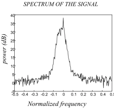
(c) (d)

Fig. 1. Cepstrum results (a) FFT spectrum, (b) cepstrum of the signal, (c) cepstrum of one echo, (d) cepstrum of the periodic term.

point. As a consequence, even with a very sophisticated al-gorithm devoted to peak identification in a spectrum, it may be difficult to separate overlapped echoes, especially when their amplitudes are very different. As an example, in UHF, if overlapped echoes could not be separated, the identified Doppler frequency may shift from clear-air to a hydrome-teor one, from altitude to altitude, from time to time, or from beam to beam. As a consequence, spurious data or no data, if using a consensus window, are obtained.

In this paper, we have investigated model-based spectral methods on simulated and actual data. These methods pro-vide the different main frequency-components present in the signal; these methods replace the peak-identification algo-rithm. The aim of this work is to point out the possibility of separating overlapped echoes directly and then to improv-ing the number of reduced data and their quality relative to Fourier spectrum analysis. The radar data came from the thunderstorm campaign that took place at the National

(3)

E. Boyer et al.: Application of model-based spectral analysis to wind-profiler radar observations 817

FIGURES

-0.5 -0.4 -0.3 -0.2 -0.1 0 0.1 0.2 0.3 0.4 0.5 0 200 400 600 800 1000 1200

-0.50 -0.4 -0.3 -0.2 -0.1 0 0.1 0.2 0.3 0.4 0.5 200 400 600 800 1000 1200

CEPSTRUM OF THE SIGNAL :

CE S

(

*

( )

f

)

SPECTRUM OF THE SIGNAL

Fig.1

Cepstrum results

Normalized frequency Fig.1.b

CEPSTRUM OF THE PERIODICAL TERM

(

)

CE

_δ

( )

f

+

_δ

(

f

−

f

0

)

Normalized frequency Fig.1.d

Fig.2

Application of the cepstrum algorithm to two

different Gaussian echoes

CEPSTRUM OF THE SIGNAL SPECTRUM OF THE SIGNAL

[image:3.595.68.251.64.238.2]

Normalized frequency Fig.2.a

Normalized frequency Fig.2.b

-0.50 -0.4 -0.3 -0.2 -0.1 0 0.1 0.2 0.3 0.4 0.5 2 4 6 8 10 12 14 16 18 20

(

)

CE S f

( )

Normalized frequency Fig.1.c Normalized frequency

Fig.1.a

-0.50 -0.4 -0.3 -0.2 -0.1 0 0.1 0.2 0.3 0.4 0.5 50 100 150 200 250 pow er pow er pow er pow er

-0.5 -0.4 -0.3 -0.2 -0.1 0 0.1 0.2 0.3 0.4 0.5 -5 0 5 10 15 20 25 30 35 40 pow er ( dB)

-0.5 -0.4 -0.3 -0.2 -0.10 0 0.1 0.2 0.3 0.4 0.5 20 40 60 80 100 120 140 pow er ( dB)

Fig. 2. Application of the cepstrum algorithm on two different Gaussian echoes.

analysis (Kay and Marple, 1981). This method is applied di-rectly to time series. Subspace-based methods are presented in the third part. The key idea consists in a decomposition of the observation space in two subspaces: the signal sub-space containing the echoes, and the noise subsub-space (Bienv-enue and Kopp, 1979, Schmidt, 1986). This decomposition is realized by computing the covariance matrix of the signal, which is then decomposed into its eigenvectors. The signifi-cant eigenvalues correspond to signal subspace eigenvectors and the other eigenvalues correspond to the noise subspace.

2 Exploitation of the power cepstrum

2.1 The power cepstrum algorithm

In the cepstrum algorithm, the power spectrum S∗(f ) is supposed to be the sum of two identical echoes,f0shifted

(Fig. 1a):

S∗(f )=S(f )+S(f −f0) (1)

s∗(t )=s(t )(1+e2j πf0t₎ ₍₂₎

wheres(t )is the Fourier transform ofS(f )ands∗(t )is the Fourier transform ofS∗(f ). Let us define the complex loga-rithm by

lnc(S)=ln|S| +iarg(S) (3)

where arg(S)represents the unwrapped phase ofSto ensure the uniqueness of the function. In the development

lnc s∗(t )₌

lnc s(t )₊

lnc 1+e2j πf0t

(4) the term lnc 1+e2j πf0t_{is a}_f

0periodical: a Fourier

trans-form of Eq. (4) exhibits a peak at the expected frequency,f0.

Consequently, the power cepstrum ofS∗(f )is defined by:

CE S∗(f )=

F TlncF T S∗(f )

= F T

lncs∗(t )

(5) whereCEdenotes the cepstrum operator andF Tthe Fourier Transform operator. (5) can be rewritten as

CE S∗(f )

=CE S(f )

+CE δ(f )+δ(f−f0) (6)

whereδ(f )denotes the Dirac distribution.

The cepstrum operator is generally applied directly on a time series, but in our case, the cepstrum operator is applied on spectra because we estimate the shift between two Gaus-sian spectra. Consequently, cepstra are represented with a “frequency” axis in Fig. 1 (b, c and d).

The second term

CE δ(f )+δ(f −f0)=F T

lnc1+e2j πf0t

of Eq. (6), represented in Fig. 1d, exhibits a peak at thef0

frequency and harmonics which are easily interpreted by the Taylor expansion of the logarithm function. In Fig. 1b, we can easily detect this peak but in some cases, the first term

CE S(f )+(represented in Fig. 1c) can hide that peak and

the estimation won’t be possible (especially when the second Gaussian echo presents a significant attenuation in compari-son with the first one).

2.2 Simulation results

For simulations, the spectrum of the signal has been com-puted as proposed by Papoulis (1965):

S∗(f )= 1

Ninc

X

m=1

St h(f )+σb2

ym 2 (7)

where St h(f )is the theoretical spectrum,σb2 is an additive noise power,Nincis the number of incoherent integration and

[image:3.595.337.521.67.223.2]

(4)

Fig.3

AR method : test on the number of pole

normalized frequency normalized frequency

pow

er (dB)

(a)

Experimental spectrum

(b) p=12

(c) p=5

(d) p=50 103

102

101

100

10-1

10-2

-0.6 -0.2 0 0.2 0.6 -0.6 -0.2 0 0.2 0.6

pow

er (dB)

pow

er (dB)

pow

er

(dB

)

-0.6 -0.2 0 0.2 0.6 -0.8 -0.2 0 0.2 1

102

101

100

10-1

102

101

100

10-1

30

20

10

[image:4.595.75.525.68.446.2]

0

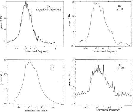
Fig. 3. AR method: tests on the number of pole (a) FFT spectrum, (b) reconstructed spectrum with a pole number of 12; (c) reconstructed spectrum with a pole number of 5; (d) reconstructed spectrum with a pole number of 50. The vertical line drawn on each plot corresponds to the 0 Hz frequency.

In Fig. 2, two different Gaussian echoes have been com-puted: the first one at zero frequency, modeling the ground clutter with a SNR of 15 dB and a normalized standard de-viation of 0,0015 and the second one, with a normalized fre-quency of−0,2, a SNR of 20 dB and a normalized standard deviation of 0,025. Even if the power cepstrum exhibits a peak at the expected frequency, the presence of numerous other peaks does not permit an immediate reliable estimation of the frequency shift.

2.3 Conclusion

As shown in the simulation, robust extraction of the shift fre-quency is not possible due to the numerous peaks. Conse-quently, this method has not been applied on actual data. In Sects. 3 and 4, a very different approach has been investi-gated which presents great improvements in relation to the

FFT algorithm. It consists of two powerful parametric meth-ods which rely on different models for the received signal.

3 Exploitation of autoregressive methods

3.1 Presentation of the method

The autoregressive (AR) spectral estimator is a standard tool in the field of spectral estimation and time series analysis (Kay and Marple,1981). AR models are often used to model data which are not necessarily generated by AR equations. For instance, high-order models are commonly used to es-timate peaked spectrum. This method is well-known for its good behaviour in resolving spectral peaks from noisy data. Given a time seriesxn, n=0,1,· · ·N−1, which is the sum of the output of an AR process,sn, and a white noise

(5)

5 10 15 20 25 30 35 40 45 50 0.024 0.026 0.028 0.03 0.032 0.034 0.036 0.038

5 10 15 20 25 30 35 40 45 50 -0.035 -0.03 -0.025 -0.02 -0.015 -0.01 -0.005

0 5 10 15 20 25 30 35 40 45 50 0.7 0.75 0.8 0.85 0.9 0.95 1 -0.5 -0.4 -0.3 -0.2 -0.1 0 0.1 0.2 0.3 0.4 0.5

-5 0 5 10 15 20 25 30 35 Fig.4.c Fig.4.b Fig.4.d Fig.4.a p p p normalized frequency pow er (dB ) FC m ean rm s

Fig.4

AR method: choice of the order p: two Gaussian echoes with f

1

=0.1

σ

1

=0.04

SNR

1

=20 dB ; f

2

=0.21

σ

2

=0.005 SNR

2

=18 dB.

m

ean

bias

(a) (b)

5 10 15 20 25 30 35 40 45 50 0.024 0.026 0.028 0.03 0.032 0.034 0.036 0.038

5 10 15 20 25 30 35 40 45 50 -0.035 -0.03 -0.025 -0.02 -0.015 -0.01 -0.005

0 5 10 15 20 25 30 35 40 45 50 0.7 0.75 0.8 0.85 0.9 0.95 1 -0.5 -0.4 -0.3 -0.2 -0.1 0 0.1 0.2 0.3 0.4 0.5

-5 0 5 10 15 20 25 30 35 Fig.4.c Fig.4.b Fig.4.d Fig.4.a p p p normalized frequency pow er (dB ) FC m ean rm s

Fig.4

AR method: choice of the order p: two Gaussian echoes with f

1

=0.1

σ

1

=0.04

SNR

1

=20 dB ; f

2

=0.21

σ

2

=0.005 SNR

2

=18 dB.

m

ean

bias

(c) (d)

Fig. 4. AR method: choice of the orderp: two Gaussian echoes withf1=0.1σ1 =0.04SN R1=20dB;f2= 0.21σ2=0.005SN R2=

18dB. (a) FFT spectrum, (b) mean bias of the estimation, (c) mean rms of the estimation, (d) spectral flatness coefficient.

and given p

X

k=0

aksn−k = −ξn a0= −1

wherewnandξnare uncorrelated white noise processes, it is well-known that

SAR(ω)=

σ_ξ2

A(ω)

2 (8)

whereσ_ξ2is the variance ofξnand

A(ω)=

p

X

k=0

ake−j ωk a0= −1 .

In the application investigated in this paper,ak will be esti-mated by solving the Yule-Walker equations using the well-known Levinson-Durbin algorithm.

3.2 Selection of the order

The first step is to determine the length of the predictor or pole numberpfor a correct representation of the spectrum.

This delicate choice is important for the frequency estima-tion, as shown in Fig. 3, where three different values of p

have been tested. In the present case (Fig. 3a), the atmo-spheric echo is stronger than the clutter one; in many cases, it is the reverse situation. p = 5 (Fig. 3c) leads to a fairly poor representation of the spectrum; in the case where an atmospheric echo is weaker than the clutter one, the atmo-spheric echo may not be present in the spectrum. p = 50 (Fig. 3d) leads to a fairly rich representation of the spec-trum with parasite peaks: it is no longer possible to safely select the right Doppler frequency. The intermediate case ofp =12 (Fig. 3b) leads to a correct representation of the spectrum.

(6)

5 10 15 20 25 30 35 40 45 50 0.005

0.01 0.015 0.02 0.025 0.03 0.035

5 10 15 20 25 30 35 40 45 50 -0.05

-0.04 -0.03 -0.02 -0.01 0 0.01

5 10 15 20 25 30

0.905 0.91 0.915 0.92 0.925 0.93 0.935 0.94 0.945 -0.5 -0.4 -0.3 -0.2 -0.1 0 0.1 0.2 0.3 0.4 0.5

-10 -5 0 5 10 15 20

Fig.5.b

Fig.5.d Fig.5.a

Fig.5

AR method: choice of the order p: two Gaussian echoes with f

1

=0.06

σ

1

=0.03

SNR

1

=10 dB ; f

2

=-0.06

σ

2

=0.03 SNR

2

=0 dB

p

p p

normalized frequency

pow

er (dB)

Fig.5.c

FC

m

ean

bias

m

ean

rm

s

(a) (b)

5 10 15 20 25 30 35 40 45 50 0.005

0.01 0.015 0.02 0.025 0.03 0.035

5 10 15 20 25 30 35 40 45 50 -0.05

-0.04 -0.03 -0.02 -0.01 0 0.01

5 10 15 20 25 30

0.905 0.91 0.915 0.92 0.925 0.93 0.935 0.94 0.945 -0.5 -0.4 -0.3 -0.2 -0.1 0 0.1 0.2 0.3 0.4 0.5

-10 -5 0 5 10 15 20

Fig.5.b

Fig.5.d Fig.5.a

Fig.5

AR method: choice of the order p: two Gaussian echoes with f

1

=0.06

σ

1

=0.03

SNR

1

=10 dB ; f

2

=-0.06

σ

2

=0.03 SNR

2

=0 dB

p

p p

normalized frequency

pow

er (dB)

Fig.5.c

FC

m

ean

bias

m

ean

rm

s

(c) (d)

Fig. 5. AR method: choice of the orderp: two Gaussian echoes withf1=0.06σ1=0.03SN R1=10dB;f2= −0.06σ2=0.03SN R2=

0dB. (a) FFT spectrum, (b) mean bias of the estimation, (c) mean of the estimation, (d) spectral flatness coefficient.

rms; in Fig. 5b and Fig. 5c, the value ofp = 12 minimizes the mean bias, but not the rms. An alternative to this classi-cal statisticlassi-cal study is to selectpaccording to the predictive noise spectral flatness. Such a spectral flatness coefficientF c

can be defined as follow (Sto¨ıca, 1997)

0≤F c= exp

" 1

2

R −1

2

ln Sn(f )

df

#

1 2

R −1

2

Sn(f )df

≤1 , (9)

whereSn(f )is the spectrum of the noise given by

Sn(f )= S f

SAR f

(10)

withS(f )as the FFT spectrum andSAR(f )as the AR spec-trum. Since this noise must be white, the pole numberpfor theAR estimation is given by the corresponding spectrum

Sn(f )which is the flattest. The flatness ofSn(f )is charac-terized by the spectral flatness coefficient previously intro-duced. As the flatness ofSn(f )increases withF c, the pole numberpfor theARestimation is given by the value which maximizesF c. The results of simulations lead to a choice of

p =13 in the first case (Fig. 4d) andp =10 in the second case (Fig. 5d). Regarding all of these results, the value of

p=12 seems to be a good choice for the various scenarios. 3.3 Experimental Results

(7)

rK r( )t

r1

r2

∆Ts ∆Ts

Fig.6

Reshaping of the autocorrelation sequence

Fig. 6. Reshaping of the autocorrelation sequence.

representative of the mean peak frequency, is computed. In some cases, although fewer than in the regular FFT spectrum method, the Doppler frequency cannot be detected because it is merged into a large echo. This case occurs when the atmo-spheric echo is very close to the clutter and relatively broad. This method, as it was implemented, cannot provide either the standard deviation or the backscattered power; using the reconstructed spectrum, they are underestimated especially whenpis small. In the data reduction process, these param-eters were obtained by means of the FFT spectrum after the identification of the mean frequency of the concerned echo. 3.4 Conclusion

The AR method, as it was implemented, improved the peak identification relative to the FFT spectrum analysis. It was an interesting method to obtain a first guess of the wind data; therefore, a peak search was no longer necessary. In our case, one of the limitations is the need to compute the spectrum in order to retrieve the other parameters, such as standard deviation and backscattered power. But further investigations will be carried out to avoid this constraint.

4 Introduction of a model-based approach for subspace parametric estimation

Different algorithms are exploiting subspace properties of covariance matrix methods (Bienvenue and Kopp, 1979, Schmidt, 1986). For simulation and experimental results, the MUSIC algorithm has been computed.

[image:7.595.307.545.61.230.2]

4.1 Application of the MUSIC algorithm to the times series MUSIC (Multiple Signal Characterization) is one of the “high resolution subspace methods”, which is well adapted to estimate spectra composed of pure lines. This was first used as an array processing to estimate the direction-of-arrival of different point sources. Our approach is original since the MUSIC algorithm is applied to the autocorrelation function of the time series. On the hypothesis of a spectrum contain-ing echoes with a relatively small standard deviation, the the-oretical autocorrelation function is considered as a sum of sinusoidal signals with a slowly varying amplitude,

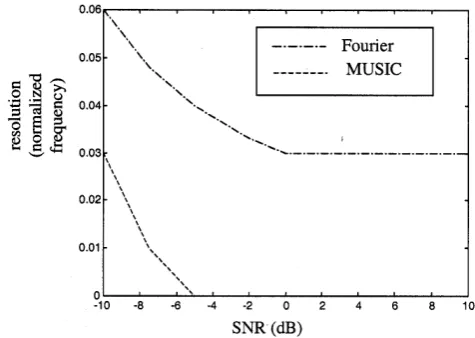
Fig. 7. Resolution of the MUSIC algorithm versus FFT algorithm.

r(t )=X i

αi(t )ej ωit.

The frequency estimation is conducted here as if the envelope was constant (the termsαi(t )are assumed to be independent oft). This hypothesis corresponds to a spectrum composed of pure lines and it leads to the use of the MUSIC algorithm. Consider anN ×1 complex vectorr(t )corresponding to the concatenation ofN autocorrelation lags. As in array sig-nal processing problem formulation, in order to obtain mul-tiple vectorial sub-observations ofr(t ), the vectorr(t )must be reshaped intoKm×1 vectorsrk, as explained in Fig. 6, whereTS is the pulse repetition time,1TS is an adjustable shift andK =int[(N−m)/1+1], where int() denotes the integer part operator. A classical eigenvalue decomposition of the covariance matrix

Rr=

1

K

X

k=1

rkrHk

is then performed to estimate the first spectral moments of Gaussian echoes and where(•)Hdenotes the Hermitian trans-pose. The influence of the temporal variation ofαi(t )on the quality of the MUSIC estimation in the case of a single echo can be found in Besson and Sto¨ıca (1996).

[1cm]

4.2 Simulation results

[image:7.595.53.290.65.153.2]

(8)

[image:8.595.60.537.333.530.2]

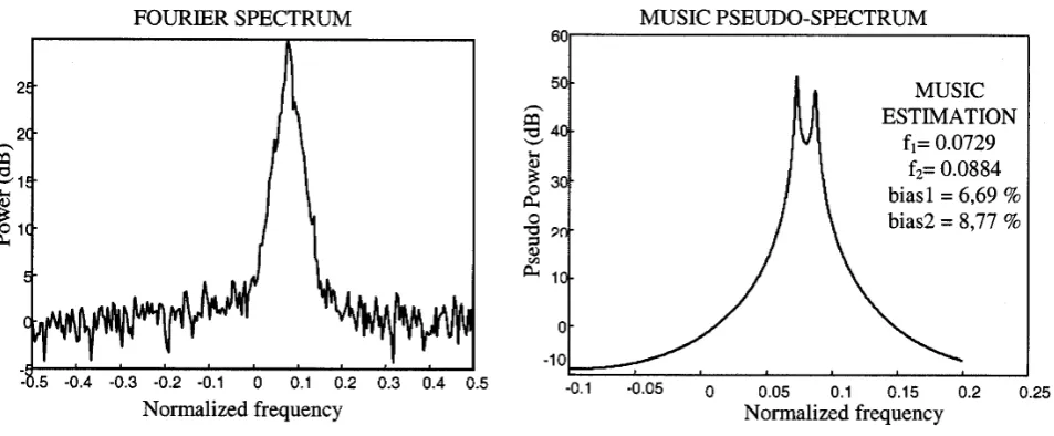
Fig. 8. Simulation example with two identical Gaussian echoesNinc = 1,SN R = 10dB,Nff t = 1024,f1 = 0.0391,f2 = 0.0586

andσ =0.01.

Fig. 9. Simulation example with two different Gaussian echoesNinc = 1,SN R = 10dB,Nff t = 256,σ1 = 0,005,f1 = 0.0781,

σ2=0,02 andf2=0.0813.

echoes, where the Fourier-like techniques lack in resolution. Moreover, one can notice that for a SNR greater than−5 dB, the resolution of the MUSIC algorithm reaches the zero limit: in this case, it is always theoretically possible to separate two echoes. With actual data, the noise and statistical fluctua-tions of the signal limit the possibility to separate very close echoes. This improvement of the resolution is illustrated in Fig. 8 and Fig. 9 where a strong overlapping has been simu-lated. In Fig. 8, considering only the spectrum, it is difficult to know whether the spectrum is composed of one or two

echoes, except if this was ascertained from time or/and alti-tude continuity. Bias and variance have been estimated with 500 Monte Carlo simulations. Clearly, an estimation of the mean frequencies is still possible in a domain where Fourier-like techniques fail.

4.3 Experimental results

(9)

[image:9.595.315.547.60.404.2]

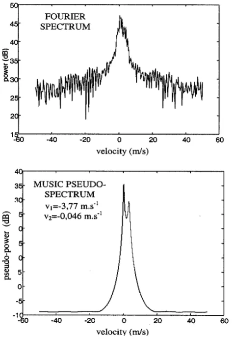
Fig. 10. Experimental results: first example.

Arecibo, PR during September and October 1998. These two examples present cases with overlapped echoes. For these two cases, MUSIC provides an estimation of the mean veloc-ity which is consistent with the Fourier spectrum. In Fig. 11, MUSIC exhibits three significant peaks where a Fourier es-timation would have some difficulties in estimating the rel-ative contribution of the ground clutter and the “negrel-ative” frequency peak. Of course, we need to pay attention to the interpretation of the results: when Gaussian echoes have a large standard deviation, MUSIC will exhibit several peaks inside that echo, thereby complicating the analysis of the re-sults. Thus, an a-posteriori analysis is necessary to interpret the different peaks obtained with MUSIC and to select the one which is representative of the atmospheric contribution. As a matter of fact, several contributions may be present in the spectrum: clear air, clutter, hydrometeor, in case of strong rain, and spurious echoes. Moreover, it is important to men-tion that the MUSIC algorithm can be implemented in real time.

4.4 Conclusion

If the standard deviation of the echo is small, subspace-based methods provide good results. Application of subspace-based

20

20 0

Fig. 11. Experimental results: second example.

methods to large standard echoes leads to poor statistical per-formances due to the inadequacy between the signal and the pure line spectra model assumed by subspace-based meth-ods. An alternative to this problem is to take into account the algorithm for both the Doppler frequency and standard deviation, conducting so to a 2D pseudo-spectrum. This is ongoing work (Boyer and al., 2001).

5 Conclusion

[image:9.595.49.287.61.406.2]

(10)

autocorrela-824 E. Boyer et al.: Application of model-based spectral analysis to wind-profiler radar observations tion function, appears to be a good alternative to Fourier-like

techniques when echoes are overlapped, with a possible real time implementation. A decisive step is to estimate the two other moments of the echoes (for a joint estimation of the three spectral moments of the echoes, see Boyer et al., 2001). The next step will be to implement this algorithm on a work station, to reduce actual data routinely and to compare with methods based on peak identification in the power spectrum.

Acknowledgement. The National Astronomy and Ionospheric

(NAIC) Center is operated by Cornell University under contract with the National Science foundation.

Topical Editor D. Murtagh thanks C. E. Meek for his help in evaluating this paper.

References

Balluet, J. C., Lacoume, J. L., and Baudois, D., Séparation de deux échos rapprochés par le cepstre d’énergie, Ann. Télécommunication, 36 n◦7–8, 1981.

Bengtsson, M. and Ottersten, B., On Approximating a Spatially Scattered Source with Two Point Sources, Proceedings of NOR-SIG’98, 45–48, 1998.

Besson, O. and Stoica, P., Analysis of MUSIC and ESPRIT Fre-quency Estimates for Sinuso¨ıdal Signals with Lowpass En-velopes, IEEE trans. On signal processing, vol. 44 n◦9, 1996 Bienvenue, G. and Kopp, L., Principes de la goniom´etrie passive

adaptative, Proc. GRETSI, Nice, 106–116, 1979.

Boyer, E., Petitdidier, M., Adnet, C., and Larzabal, P., Subspace-based spectral analysis for VHF and UHF radar signals, Proc. PSIP, 385–390, 2001.

Chen, W., Zhou, G., and Giannakis, B., Velocity and accelera-tion estimaaccelera-tion of Doppler weather radar/lidar signals in colored noise, Proc. ICASSP95, 2052–2055, 1995

Fournel, T., Daniere, J., Moine, M., Pigeon, J., and Courbon, M., Utilisation du cepstre d’énergie pour la vélocimétrie par images de particules, Traitement du signal vol.9-n◦3, 1992

Hocking, W. K., System design, signal processing and preliminary results for the canadian VHF atmospheric radar, Radio Sci., 32, 687–706, 1997.

Kay, S. and Marple, S. L., Spectrum Analysis-A modern Perspec-tive, Proc. IEEE vol. 69 n◦11, 1380–1419, 1981.

Oppenheim and Shafer, Digital signal processing, Prentice Hall 481–528, 1989.

Papoulis, A., Probability, Random Variables and Stochastic Pro-cesses, New York, MacGraw- Hill, 1965.

Petitdidier, M., Ulbrich, C. W., Laroche, P., Campos, E. F., and Boyer, E., Tropical thunderstorm campaign at Arecibo, PR, in. Proceedings of the ninth workshop on technical and scientific aspects of MST radar and combined with COST-76 final pro-filer workshop, Toulouse, March 13–18, 2000. Editor: Belva Edwards. Scostep secretariat, NOAA,325 Broadway, Boulder, CO80303 USA.

Sato, T. and Woodman, R. F., Spectral parameter estimation of CAT radar echoes in the presence of fading clutter, Radio Sci., 17, 817–826, 1982.

Schmidt, R. O., Multiple emitter location and signal parameter es-timation, IEEE Trans. on Antenna and propagation, vol 34 n◦3, 276–280, March 1986.

Sto¨ıca, P. and Moses, R., Introduction to spectral analysis, Prentice Hall, 1997.

Tsuda, T., Data acquisition and processing, International School on Atmospheric radar, in Handbook for MAP, 30, pp 151–184, SCOSTEP Secr., University of Illinois, 1406W Green Street, Ur-bana, Ill. 61801, USA, 1989.

References

Balluet, J. C., Lacoume, J. L., and Baudois, D., S´eparation de deux ´echos rapproch´es par le cepstre d’´energie, Ann. T´el´ecommunication, 36 n◦7–8, 1981.