TECHNICAL NOTE
OPTIMIZATION OF LONGWALL PANEL LOCATION WITH
REGARDS TO THE GRADIENT OF COAL SEAMS
K. Oraee
Department of Mining Engineering, University of Tarbiat Modares Tehran, Iran, [email protected]
(Received: December 1, 2000 – Accepted in Revised Form: October 3, 2002)
Abstract The paper begins by outlining the role and importance of coal as a source of energy and in the steel industry. It briefly describes the longwall method of working together with the conventional machinery used in the method. A mathematical model is then proposed that shows the relationship between the gradient of the coal seam, that of the face and the entries to the panel. Determination of a model that mathematically shows the economically best location for the longwall panel with regards to the seam gradient is the core section of the paper which is accomplished by introducing an objective function and devising its component models. The model is then subjected to sensitivity analysis. The results can assist the mining engineer in determining the most economic location for the longwall panels.
Key Words Coal, Longwall, Face, Steep Seam Panel, Face Direction
ﻩﺪﻴﻜﭼ
ﻩﺪﻴﻜﭼ
ﻩﺪﻴﻜﭼ
ﻩﺪﻴﻜﭼ
ﺭﻮﻄﺑ ﻩﺩﻮﻤﻧ ﻩﺭﺎﺷﺍﻱﮊﺮﻧﺍ ﻢﻬﻣ ﻊﺒﻨﻣ ﻚﻳ ﻥﺍﻮﻨﻋ ﻪﺑ ﮓﻨﺳ ﻝﺎﻏﺯ ﺖﻴﻤﻫﺍ ﻭﺶﻘﻧ ﻪﺑ ﺍﺪﺘﺑﺍﺮﺿﺎﺣ ﻪﻟﺎﻘﻣ
ﻪﻬﺒﺟﺵﻭﺭﻪﺻﻼﺧ
ﻲﻣﺢﻴﺿﻮﺗﺍﺭﻥﺁﺭﺩﻩﺩﺎﻔﺘﺳﺍﺩﺭﻮﻣﺕﻻﺁﻦﻴﺷﺎﻣﻭﻲﻧﻻﻮﻃﺭﺎﻛ ﺪﻫﺩ
. ﻲﺿﺎﻳﺭﻝﺪﻣﻚﻳﺲﭙﺳ
ﻞﻧﻮﺗ،ﺭﺎﻛ ﻪﻬﺒﺟﻂﺧﻲﻘﻴﻘﺣﺐﻴﺷ ﻦﻴﺑﻪﻄﺑﺍﺭﻪﻛ ﻩﺪﺷﻪﺋﺍﺭﺍ
ﻝﺎﻏﺯﻪﻳﻻﻲﻠﻛﺐﻴﺷﻭﻥﺁﻑﺮﻃﻭﺩ ﻲﺳﺮﺘﺳﺩﻱﺎﻫ
ﻲﻣﻥﺎﺸﻧ ﺍﺭﮓﻨﺳ ﺪﻫﺩ
.
ﻲﻣﻥﺁﺯﺍﻩﺩﺎﻔﺘﺳﺍﺎﺑﻪﻛ ﺖﺳﺍﻲﺿﺎﻳﺭ ﻝﺪﻣﻚﻳﻪﺋﺍﺭﺍ ﻪﻟﺎﻘﻣﻲﻠﺻﺍﺖﻤﺴﻗ ﻥﺍﻮﺗ
ﻱﺩﺎﺼﺘﻗﺍ
ﻳﺮﺗ ﻦ
ﺩﺭﻭﺁﺖﺳﺪﺑﺍﺭﻲﻧﻻﻮﻃﺭﺎﻛﻪﻬﺒﺟﻪﻧﻮﻤﻧﻪﻨﻬﭘﻚﻳﻱﺮﻴﮔﺭﺍﺮﻗﻞﺤﻣ .
ﻊﺑﺎﺗﻚﻳﻒﻳﺮﻌﺗﺯﺍﻩﺩﺎﻔﺘﺳﺍﺎﺑﻝﺪﻣﻦﻳﺍ
ﺖﺳﺍﻩﺪﻣﺁﺖﺳﺪﺑﻲﻘﻴﻘﺣﺩﺍﺪﻋﺍﺯﺍﻩﺩﺎﻔﺘﺳﺍﺎﺑﻥﺁﻩﺪﻨﻫﺩﻞﻴﻜﺸﺗﻱﺍﺰﺟﺍﻪﺒﺳﺎﺤﻣﻭﻑﺪﻫ .
ﻲﻣﺍﺭﻖﻴﻘﺤﺗﻦﻳﺍﺞﻳﺎﺘﻧ
ﺮﺑﺭﺎﻜﺑﮓﻨﺳﻝﺎﻏﺯﻱﺎﻫﻪﻳﻻﻲﺟﺍﺮﺨﺘﺳﺍﻱﺎﻫﻲﺣﺍﺮﻃﺭﺩﻥﺍﻮﺗ ﺩ
.
1. INTRODUCTION
Energy is considered to be one of the most important factors contributing to economic growth. Despite short-term fluctuations and geographical variations regarding the global demand for energy, coal has been a primary source of energy for centuries and its total world output has always had an increasing trend. The increase in total production has been brought about, more than anything else, by the application of more efficient methods and machinery. Longwall method is relatively new in many countries. It has always been predominant in the U.K coal mining industry but its full potentials as regards
production levels, mechanizability and productivity were realized by the American coal mining industry and others, in the latter part of the twentieth century. It is now the most widely used underground coal mining method in many parts of the world.
Each of these sections has certain duties to perform:
1. The coalface is conventionally equipped with a number of powered supports or hydraulic props; one or more cutter/loaders, such as shearer loader, plough, etc; and a type of armored flexible conveyor (AFC) for transporting the coal from the face to the main entry.
2. The main entry is the roadway through which coal is transported out of the panel area, by means of a usually fixed belt conveyor to the trunk roadway.
3. The tail entry could be considered as a store for electrical, control and ancillary equipment as well as means of providing through ventilation.
Coal seams of 3.5m thick with the gradient of 0-45° could be considered suitable for longwall mining, although continuity of the seam and the nature and characteristics of its roof and floor can have important bearing on the application of the method.
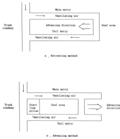
Longwall panels of 700-1500m long and 100-250m wide are now most common. Coal from these panels is won either by advancing or retreating system of working (Figure 2).
One of the attractions of the longwall method is its applicability in seams with higher gradients. Since all the developments are driven within the coal seam, the gradient of the face and that of the entries change with changes in the location of the panel. The total cost of winning the coal in the panel also changes accordingly and it is the intention of this paper to find the optimum gradient for the face and hence that for the entries, so that the total
cost will be at minimum.
2. RELATIONSHIP BETWEEN THE GRADIENT OF THE FACE, ENTRIES AND
THE COAL SEAM
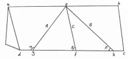
A typical face with two entries (single entry) is assumed. The face line is also assumed to be perpendicular to the direction of the entries and therefore any rotation of the panel within the seam increases the gradient of one, while decreasing that of the other. For example, if the panel is rotated in a way that face gradient is decreased, then the gradient of the entries increases; and ultimately the face is level (zero gradient) when the gradient of the entries is equal to the seam full dip. The maximum dip for each of these is therefore equal to the seam full dip and the minimum is zero. To obtain a relationship between these, a part of the coal seam, such as “abcd” plane (Figure 3) is considered.
The two lines “eg” and “eh” show the gradients of the face and of the entries respectively. These
Figure 1. A typical longwall panel.
two lines are within the “abcd” plane and are perpendicular to each other. They also form gradients of “α” and “β” respectively, with the horizontal plane. Using the drawing in fig 3, the length of the three lines “eg”, “eh” and “ef” can be defined as follows:
α = =
sin 1 A
eg (1)
β = =
sin 1 B
eh (2)
γ = =
sin 1 C
ef (3)
On the other hand, the angle at “h” is common between triangles “egh” and “feh” and the two angles “geh” and “efg” are equal (both 90°). The two triangles “egh” and “efh” are therefore similar and hence:
gh B B fh A C
=
= (4)
Or
C BA D
gh= = (5)
Also in triangle “egh” we have:
A2 + B2 = D2 (6)
Combining the two Relations 5 and 6, it is concluded
that:
2 2
2
C BA B
A
=
+ (7)
Or
2 2
2 C
1 A
1 B
1
=
+ (8)
If the values of A, B and C are now substituted in this equation, we will have:
sin²α + sin²β = sin²γ (9)
This equation shows the relationship between the gradient of the coalface (α), that of the two parallel entries (β) and the seam full dip (γ).
3. OPTIMISATION OF PANEL LOCATION WITH RESPECT TO DIP
The intention here is to find the optimum location of the longwall panel, that is, where the total cost of the development and coal extraction in the typical panel is minimum. For this purpose, the objective function Cт is defined as follows:
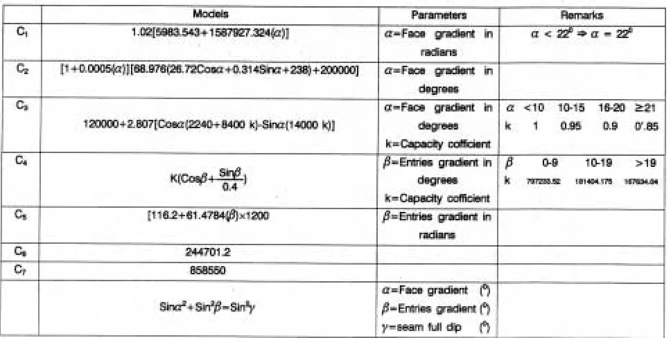
Cт = C1+ C2 + C3 + n (C4 + C5) + C6 + C7 (10) Where:
• CT is the total cost of exploitation of the panel, • C1 is the costs associated with the face
supports,
• C2 is the shearer loader costs, • C3 is the AFC costs,
• C4 is the total support costs of the two entries, • C5 is the cost of driving the two entries, • C6 is coal transportation cost in the main entry, • C7 is all other panel costs, such as ventilation,
lighting, drainage, communication etc,
• n is the number of entries serving the panel, which will be equal to 2 in a single entry system.
Individual models will therefore have to be devised for C1-C7 in order to evaluate CT, the total cost of the panel. For this purpose, a typical panel is
considered with most common parameters. Since, amongst all external variables, the gradient is of interest here, at this stage, all other parameters are assumed constant.
4. ASSUMPTIONS
1) Panel type: single entry, retreat face 2) Seam thickness: 2 meters
3) Seam full dip: 40°
4) Panel dimensions: 1200m × 200m 5) Powered supports capacity: 240-450 tons 6) Coal cutting is carried out by one shearer loader,
DERDS, 250-500 KW
7) Coal transport is carried out by AFC, width 762mm
8) Both roof and floor are sandstone or some other competent material
9) Three 8 hour shifts are performed per day 10) Steel frame support system is used throughout
the entries
11) Coal transport in the main entry is carried out by 800mm wide belt conveyor.
5. POWERED SUPPORTS COST
As the gradient of the face varies, the magnitude of the load exerted upon the roof changes and with that the capacity of powered supports will have to be different. This in turn makes powered supports costs vary with the face gradient.
To determine the magnitude of the force exerted on the roof, Wilson formula has been used [1]. This states:
+ δ
ψ α γ = cos tan sin H
F (11)
Where:
• F is the average density of the load exerted on the face (ton/m²).
• γ is specific gravity of the immediate roof (tons/m³).
• H is thickness of the immediate roof (m). • α is the face gradient (degrees).
• δ is the seam full dip (degrees).
• ψ is the angle of friction between the immediate roof and the main roof.
The roof material is assumed to be sandstone, therefore:
γ = 2700(tons/m³) δ = 40° tan ψ = 0.4 Hence the magnitude of the load is calculated by:
) m / tons ( 766 . 0 4 . 0 sin 10 32 . 1
F 3 2
α+
×
= − (12)
On the other hand, we have the following formula for designing powered supports for such a face [2]:
le 102
W . F
Psa = Psn = η . Psa Pyn = λPsn Py = 102 Pyn.le.s
(13) Where:
• W is the width of the immediate roof (m) • le is the length of the canopy (m)
• Psa is the active static stress on the support (MPa)
• Psn is the nominal static stress (MPa) • Pyn is the nominal yield stress (MPa)
• η is the correction coefficient, which is equal to 1.25 • λ is a constant equal to 1.25
• S is the center distance between powered support sets • Py is the capacity of powered supports (tons) Since it is assumed that the powered supports used are of the shield type, it can be deduced that W=5.6m and le=3.5m.
Therefore: s 5 . 3 766 . 0 4 . 0 sin 10 24 . 3 102
Py 5 × ×
α +
× ×
= −
(14) Now if the capacity of one set of powered support
is known, for example 250 tons and if the face length is 200m, we have [3]:
α +
=
= 0.766
4 . 0 sin 94 S 200
N (15)
powered support sets.
In this way the numbers of powered support sets are calculated. We now assume that the useful economic life of a powered support set allows the set to be used on six consecutive panels and also that the whole length of the roof is covered by powered supports. Also considering the price range of US$ 18,480 for supporting each meter of the face length in the case of 6-leg 240 tons sets to US$ 33,280 in the case of 4-leg 450 tons sets, we can deduce [4]:
C1 = 1.02 [5983.542 + 587927.324 (α)] (16) Where:
• C1 is the total powered support cost in US Dollars • α is the face gradient in radians
This relation holds for 22°≤α≤40° and if α≤22° then its value is assumed to be equal to 22°.
6. CUTTING/LOADING COSTS
For the seam assumed to be 2m thick here, it is considered that one Double Ended Ranging Drum Shearer (DERDS) unit is suitable and its total costs will be:
Total cutting/loading costs = Capital cost + Operational costs
The price of one unit of such shearer loader is assumed to be US$ 1,200,000 and that during its economic life; it should be able to serve six panels. The capital cost of such shearer loader is therefore US$200,000 per year. The total power cost of the shearer loader can be calculated from:
Total power Pt = (P1 + 340) + P2 (17) Where:
• P1 is the power consumption when cutting (down the slope)
• P2 is the power consumption when flitting (up the slope)
• 340 is the power used to rotate the drums, which is constant
We now expand P1 and P2 and the power consumption is analyzed with regard to its normal
and horizontal components. Also the weight of a DERDS unit is assumed to be 20 tons and its cutting and flitting speed are assumed to be 4.7 and 14.1 meters per minute respectively. We then have [4]:
P1 = 26.72 cos α + 0.314 sin α + 238 (KWh) (18) P1 is the power consumption when the shearer loader is running, i.e. either cutting or flitting. Combining this relation with that for the total number of cuts, we have:
1 p f. s . n P
η
= (19)
Where:
• n is the total number of cuts in a panel, assumed to be 1,437
• s.f is the safety factor, assumed to be 1.2 • η is the technical efficiency of shearer loaders,
taken to be 0.8 We therefore have:
C = 200,000 + 68.976 (26.72cos α + 0.314sin α + 238)
(20) In this model, the angle α is measured in terms of
degrees and C measures the total power cost. Adding the miscellaneous power costs, cost of idle periods etc, we have [4]:
C2 = [(1 + 0.0005(α)] [200,000 +68.976 (267 cos α + 0.314 sin α + 238) US$
(21)
7. COAL TRANSPORT COSTS AT THE FACE
When the face gradient varies, the power required to transport coal along the face also varies. With this variation, the cost of coal transport increases with the gradient of the face line. To calculate the AFC power consumption, the forces against motion of the AFC are analyzed.
Fc = Ws.L(cos α.µs + sin α) + Wc.l(cos α.µs – sin α) Full
(23) Where:
• Fs is the force required to move the empty AFC up the slope
• Fc is the force required to move the full AFC down the slope
• Ws is weight of unit length of the AFC (kg) • Wc is weight of the coal loaded on unit length of
the AFC (kg)
• µs is the AFC friction coefficient • µc is the loaded AFC friction coefficient • L is length of the AFC (m)
• α is the face gradient (degrees)
Total force required for one cut is therefore:
Ft = 1.1 (Fc + Fs) (24)
If we now take L=200m, µs=0.4, Ws=14 kg/m, K=capacity coefficient, µc=0.6, Wc=70kg/m and adding to these the facts that there will be 1,437 cuts needed for the total extraction of such panel, each cycle of the AFC takes 0.0855 hours and also that there will be 34 cycles for the AFC in each cut, we will have [4]:
P=58.483[cos α (2240+8400K) – sin α (14000K) (KWh)
(25) If we now take US$ 120,000 to be the capital cost
of the AFC, assume the cost of energy to be US$ 0.032/kwh and the reciprocal of the efficiency of the AFC motors to be 1.2, we then have:
p 8 . 0 2 . 1 032 . 0 000 , 120
C3 = + × × (26)
Or
C3 = 120,000+2.807 [cos α (2240 + 8400K) – sin α (14000K) US$
(27) Capacity coefficient (K) 1 0.95 0.9
0.85
Face gradient (α) <10° 10°-15° 16°-20° >20°
8. ENTRIES’ SUPPORT COSTS
The magnitude and characteristics of the load exerted on the roof and sides of the access entries vary with the gradient of these entries. The entries support system is therefore designed to suit the gradient of these entries and their support cost therefore depends on the gradient of these entries. According to rock mechanics principles [3] the intensity of the load applied on horizontal entries could be calculated using Equation 28:
qt = α .L.γ.a (28)
This equation can be made applicable to dipping roadways: ) 4 . 0 sin (cos a . . L .
qt=α γ β+ β (29)
Where:
• qt is intensity of the uniform load on the roof (ton.m) • α is coefficient of load condition (normal
condition = 0.5)
• L is length of the support canopy (m)
• γ is specific gravity of the immediate roof (tons/m³) • a is the distance between each two powered
support units (m)
Now if we substitute L=2.5m and γ=2.7 tons/m³, then: ) 4 . 0 sin (cos a 7 . 2 5 . 2 5 . 0
qt= × × × α+ α (30)
On the other hand, for beams of types Gl 120, Gl 130 and Gl 140, we have:
| σ | = 3375.657 qt≤14000 Therefore qt≤4.147 Substituting for the above equation we will have:
147 . 4 ) 4 . 0 sin (cos a 375 .
3 × β+ β ≤ (31)
If the price of powered support sets are also taken into account [5] then
) 4 . 0 sin (cos 52 . 197233 C 0
) 4 . 0 sin (cos 174 . 181404 C
20 10
If ≤β≤ = β+ β $
) 4 . 0 sin (cos 04 . 167634 C
20
If β≥ = β+ β $
Or
) 4 . 0 sin (cos K
C4 = β+ β $
9. ENTRIES’ DRIVAGE COSTS
Driving inclined headings are generally expected to be more expensive than horizontal ones. In this case, headings with a cross section area of 6m² are considered appropriate and using data from the USBM the relation that shows this type of costs is found to be [6]:
C5 = [116.2 + 61.4784 (β)] × 1200 (32)
Where:
• C5 is the cost of entries’ drivage in $US,
• β is the gradient of the entries in radians
10. TRANSPORT COSTS IN THE MAIN ENTRY
The cost of transporting coal in the main entry does not vary much with changes in the gradient of the entry itself, and is found to be [2]:
C6 = 244,700 $ (33) Where C6 is the transport cost of coal in $US.
11. MISCELLANEOUS COSTS
All other costs, lighting, ventilation, communications, etc are considered here and found to be unrelated to face and entries gradient and therefore assumed
constant [7]:
C7 = 858,500 $
Where C7 is the total miscellaneous costs in $US.
12. OPTIMUM LOCATION OF THE PANEL
Combining the models for C1 to C7, the model for CT, the total cost of the panel will be deduced, as follows:
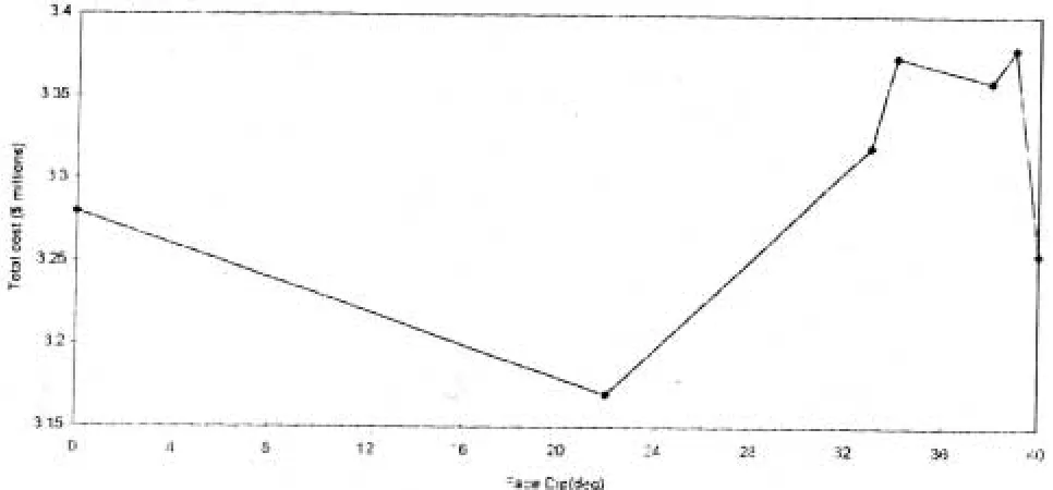
CT = C1 + C2 + C3 +2(C4 + C5) + C6 + C7 The above models are summarized in table 1. The graph shown in Figure 4 shows the total cost of developing the typical panel, at different gradients of the face and hence that of the entries’. This graph shows that the minimum cost of developing the panel occurs when the face line dips at 22 degrees.
13. GENERAL MODEL
The procedure described shows how to locate
longwall panels with respect to dip, so that the total cost is minimum. In other words, the seam gradient and consequently those of the face and the entries’ vary while all other parameters are kept constant. If other variables are allowed to change simultaneously, we could obtain models for other panels that have different characteristics from the typical panel assumed earlier. For this purpose some variables have been added to the original model and therefore the general model has been devised as follows: CT = S1C1…S5C1 [C1] + S1C2…S5C2 [C2] + S1C3…S5C3 [C3] + S1C4…S5C4 [C4] × 2 + S1C5…S5C5 [C5] × 2 + S1C6…S5C6 [C6] + S1C7…S5C7 [C7]
S1C1…S1C7 are sensitivity coefficients with respect to panel length (original panel length is 1,200m) S2C1…S2C7 are sensitivity coefficients with respect to face length (original face length 200m)
S3C1…S3C7 are sensitivity coefficients with respect to seam thickness (original seam thickness is 2m) S4C1…S4C7 are sensitivity coefficients with respect to seam gradient (original seam gradient is 40°) S5C1…S5C7 are sensitivity coefficients with respect to the cost of energy (original energy cost is assumed to be 0.30 $US per KW hours).
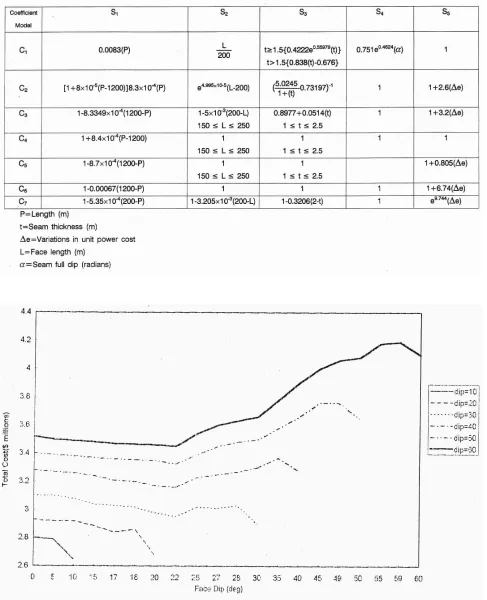
TABLE 2. Sensitivity Coefficient Models.
The resulting models for sensitivity coefficients are summarized in Table 2.
14. CONCLUSIONS
Since the variations in seam gradient are of primary interest here, the general model is subject to sensitivity analysis with respect to variations of seam gradient, that is, the coefficient S. The graphs of Figure 5 are hence obtained. Figure 5 shows that when the seam gradient is higher than 50 degrees (steep seams), an alternative route to finding optimum panel location has to be adopted. This implies that in such cases other methods of working than longwall should be applied.
It is concluded that if the seam full dip is less than 30 degrees, as is shown on the graph of Figure 5, it is most economical to design the panels in a way that full gradient is transferred to the face and the entries are near horizontal. If, on the other hand the seam dips at 30-50 degrees, it is most economical that the gradient is divided between the face and
the entries. For this purpose the model introduced earlier could be used to determine the exact position of the panel.
The model and the analyses described could prove useful in planning and development of longwall panels.
15. REFERENCES
1. Deepak, D., “Longwall Face Support Design – A Microcomputer Model”, Journal of Mines, Metals and Fuels, March (1986).
2. Peng, S. S. and Chiang, H. S., “Longwall Mining”, John Willey & Sons, New York, (1984).
3. Goodman, R. E., “Introduction to Rock Mechanics”, New York: Wiley, New York, (1986).
4. U.S. Bureau of Mines, Cost Estimating System Handbook, Edited by A. Misra, (1987).
5. Robert, B. H., “A Review of the Performance of Various Powered Supports Types”, Mining Science and Technology, New York, (1990).
6. Bickel and Kuesel, Tunnel Engineering Handbook, VNB, Vol. 68, (1982).
7. U.S. Longwall Census, Coal Journal, Vol. 16, (1993),