Perfect Tracking of Supercavitating Non-minimum Phase Vehicles Using a New Robust and Adaptive Parameter-optimal Iterative Learning Control

Please cite this article as: M. Yahyazadeh, A. Ranjbar Noei, Perfect Tracking of Supercavitating Non-minimum Phase Vehicles Using a New Robust and Adaptive Parameter-optimal Iterative Learning Control. International Journal of Engineering (IJE) Transactions A: Basics, Vol. 27, No. 7, (2014): 1071-1080

International Journal of Engineering

J o u r n a l H o m e p a g e : w w w . i j e . i r

Perfect Tracking of Supercavitating Non-minimum Phase Vehicles Using a New

Robust and Adaptive Parameter-optimal Iterative Learning Control

M. Yahyazadeh, A. Ranjbar Noei*

Faculty of Electrical Engineering, Noshiravani University of Technology, Babol, Iran,

P A P E R I N F O

Paper history: Received 24 June 2013

Received in revised form 29 October 2013 Accepted 07 November 2013

Keywords:

Iterative Learning Control Convergence

Supercavitating Vehicle Model

A B S T R A C T

In this manuscript, a new method is proposed to provide a perfect tracking of the supercavitation system based on a new two-state model. The tracking of the pitch rate and angle of attack for fin and cavitator input is our aim. The pitch rate of the supercavitation with respect to fin angle is found as a non-minimum phase behavior. This effect reduces the speed of command pitch rate. Control of such non-minimum phase in a specific time interval and improving the speed response with respect to fin control reaction is still an open problem. To overcome the problem a feed-forward control is proposed to apply on the cavitator as a control in the feed-forward configuration. The idea of this paper is to provide a certain signal for the cavitator in order to improve the tracking performance in presence of uncertainty using iterative learning control. Moreover, this paper proposes a new method based on parameter-optimal iterative learning control to solve a perfect tracking problem of systems for indefinite (not sign-definite) system. This technique provides an updating control law through applying adaptive Lyapunov gain for monotonic zero convergence of tracking error in sense of 2-norm. The simulation results verify performance and robustness of the proposed modification of iterative learning control in comparison with classical controller of the supercavitating vehicle.

doi:10.5829/idosi.ije.2014.27.07a.08

1. INTRODUCTION1

Velocity of underwater vehicles is extremely constrained by friction. But, in rigid conditions, super cavitation can separate liquid flow through the gas emanating from nose and thus decrease the drag between the vehicle and the liquid. Thus, the possibility of obtaining high velocities is provided for the vehicle and the cavity number is calculated using the following equation [1].

0 2 ₂.

c

P P

V s

r

-= ₍₁₎

where P₀ is static pressure contrary to liquid flow, Pc

pressure of cavity, r liquid density and V vehicle velocity. At high velocities, real supercavitation phenomenon will occur; but, at low velocities, another mechanism is needed to produce this phenomenon. Producing this phenomenon at high velocities

1_{*Corresponding Author Email: [email protected] (A. Ranjbar)}

considerably changes dynamics of the vehicle because contact with the confining liquid only exists in the nose (of the cavitator) and on each of the control surfaces [2]. Control surfaces are the fins that produce lift and moment forces necessary for the control and are symmetrically placed. A series of these fins is used for affecting longitudinal dynamics and are called elevators. Another fin called radar is used for affecting latitudinal dynamics. Coupling between these two dynamics is usually thought to be negligible [3]. However, non-minimum phase behavior of vehicle exists in pitch or yaw channel using fin inputs.

The lift force generated by fins helps to provide better band width and more limit disturbances. On the one hand, the adequate force needed for controlling underwater vehicle cannot be provided solely from supercavitation phenomenon, and lift and fin moment forces are also necessary; therefore, control fins are needed for the vehicle. On the other hand, the non-minimum phase behavior of vehicle exists in the pitch (or yaw) rate of fin inputs, which leads to slow reaction

of the system to the fin input and limits efficiency [4]. Disturbance mortality is slight and limited in this situation which will limit tracking. To compensate for this situation, a cavitator can be used, which provides enough force for feed-forward control in order to compensate for the slow reaction of fin's non-minimum phase behavior in the output [5].

The existence of a cavitator in supercavitating vehicles supplies the feed-forward force necessary for compensating the non-minimum phase behavior of the vehicle, which can be an advantage for supercavitating vehicles over other non-supercavitating underwater ones; this advantage is the control necessary for solving the problem of non-minimum phase behavior of the system. The exact amount of this control can be calculated using iterative learning control (ILC) which will provide a new space for solving the problem of calculating feed-forward control in order to compensate for the slow reaction. This technique is widely used in different applications such as those listed by [4-6]. The modified ILC is used to control supercavitating vehicle for the first time. ILC is an efficient controlling tool for improving transient state and efficacy of tracking in systems. The systems which work within ILC framework act repetitively by nature. Using ILC is not limited to this case, but includes all the cases in which repetition can help to obtain the desired dynamic of even a part of the system dynamics (see [7, 8]). So, repetition may depend on time, state, trajectory, etc. or their combination. On the other hand, in different studies, repetition has different concepts such as trials [9], passes [10] or iterations [11]. Although control theory provides many designing tools for improving response of dynamic system, given the un-modeled dynamics or parametric uncertainties, which occur during the operation of a real system, or lack of appropriate designing techniques, obtaining the desired performance is usually challenging [12]. Thus, it will not be easy to obtain perfect tracking using control theory. ILC is a new complement for control areas which may be useful in solving some conventional feedback design problems (like adaptive, robust, PID and other controllers) [13]. On the other hand, it has been proven that ILC is very effective for controlling minimum phase systems because of using non-causal filters. In the conventional control theory, if the system is non-minimum phase, perfect tracking will not be possible using causal filters [14-16].

In the ILC algorithm, as the number of iterations is increased, tracking error would decrease in a given time interval. Iterative learning control is a functional approach for improving efficiency of tracking and transient response, in which the control input in the current iteration is calculated through inputs and tracking errors in past iterations. In fact, the main viewpoint of iterative learning control is that it uses

information of past trials. This trend is done for improving control efficiency so that tracking error decreases in subsequent iterations.

Some of the primary studies in this regard can be seen in [17, 18]. In 2003, Owens and Feng for the first time invented a new optimal method for obtaining the input that had many advantages over conventional ILC methods including simple designing and other considerations of scientific implementation [19] and [20]. Nevertheless, making perfect tracking (convergence of tracking error to zero) largely depends on plant transfer function G. If the sign-definite condition is not satisfied in the system (sign-definite means _{G G+} T_>0 _{or G G+} T_{<0,G is a matrix of}

Markov parameters), then convergence of error to zero (as a norm) does not occur [21]. In other words, the sufficient condition for obtaining perfect tracking is that system G _{is sign-definite, which is a very constraining} condition because a vast range of systems might lack the mentioned condition. In [19], two methods were proposed for monotonous convergence to zero for indefinite systems which included using adaptive weights and exponential function. In literature [20, 21], inverse non-causal functions and system transpose system were used to provide monotonous convergence to zero tracking error for some systems. In [22], by using high order iterative learning mode control and adding special basis functions in the control input, it was shown that these basis functions could be chosen so that sign-definite condition of ideal system was satisfied. Nevertheless, an alternative method can be used to somehow improve parameter optimization so that sufficient conditions for convergence to zero could be more constrained.

In the present study, a novel updating rule was proposed using adaptive compensation learning gain strategy, in which learning gain in every iteration was updated so that the system would be sign-definite. Thus, monotonic convergence of tracking error to zero was guaranteed. This strategy is based on the point that learning gain was updated in every iteration so that the adaptive Lyapunov (Riccati) equation became as follows:

(1)

T T

j j d

GX +X G = -Q

d

2. PROBLEM of TRACKING PITCH RATE OF SUPERCAVITATING VEHICLE

In this section, first, a new model of supercavitating vehicle is briefly presented. In the next section, problem of pitch rate tracking of the vehicle is presented.

The longitudinal motion equations of a supercavitating vehicle can be reduced to a two-state longitudinal model: attack angle (α) and pitch rate (q) are stated as radiant and radiant per second 2. The new model which was obtained in this study considered thrust, gravity and fin forces in addition to the forces and moments of the vehicle under non-planning conditions of cavitator forces and used the results of [23, 24] in this regard. For this purpose, Newton laws were used to rewrite motion equations through forces (F ) and moments (M) applied to the vehicle as follows:

(2)

(

)

1

.

x x x x

c T g

u F F F F wq

m d = + + + -& (3)

(

)

1

z z z

c g

w F F F uq

m d = + + + & (4)

(

)

1 _. y y c yy

q M M

I d

= +

&

in which indexes c, T, g _and d _{show cavitator, thrust,} gravity and fin angle, respectively. Also, u _and w _are components of linear speeds of the vehicle in body coordinates and show pitch rate q (rotation rate around y _{axis) in the direction of} xand y _{axes of the vehicle.} Also, m and Iyy are mass and moment of inertia,

respectively. Supercavitating vehicle has usually constant linear velocity in the direction of x axis [1]; in other words, u&=0. Using attack angle of the vehicle,

i.e.a&»( ) ( )w& u , and also using the Taylor expansion,

the model is reduced to two state, in which case the following relations show longitudinal motion equations of system in the vehicle [1].

(5)

(

)

1

z z z

c g

F F F q

mu d

a&= + + +

(6)

(

)

1 . y y c yy

q M M

I d

= +

&

in which terms F_dzand M_dzare as follows:

(7)

(

2

)

z L fin e fin

F_d = -rc S_a ud +u w x uq

-(8)

(

2

)

y L fin fin e fin

M_d =rc S x_a ud +uw x u q

-fin

x , r, S_finand cLaare respectively distance of mass center to fin, liquid density, fin surface and the

coefficient resulting from changes of lift coefficient with respect to attack angle.

2. 1. Linearization and Trim Conditions Equations (5) and (6) show vehicle model with two dynamic and nonlinear states in longitudinal axis which are presented in terms of force and moment for the cavitator, gravity and fin. By placing a& &,q=0, trim points are obtained [1]. Nonlinear equations can be converted into linear ones about trim points or working points. Thus, the new two-state equation is linearized as follows: (9) 1 1 1 1 1 1 1 1 1

z z z z

y y y y

z z y y c c c c yy yy c c e c

yy c yy e

F F F F

mu mu q q

M M M M q

q

I I q q

F F mu mu M M I I d d d d d d a a a a a a d d d d

é æ¶ ¶ ö æ¶ ¶ ö ù

+ + +

ê ç_{¶ ¶} ÷ ç_{¶ ¶} ÷ ú

è ø è ø

é ù₌ê ú é ù

ê ú ê _{æ¶ ¶ ö æ¶ ¶ ö ë û}ú ê ú

ë û ê _{ç + ÷ ç + ÷}ú

ç ÷ ç ÷

ê _{è ¶ ¶ ø è ¶ ¶ ø}ú

ë û

¶ ¶

æ ö æ ö

ç_¶ ÷ ç_¶ ÷

è ø è ø

+

¶ ¶

æ ö æ ö

ç ÷ ç ÷

ç_¶ ÷ ç_¶ ÷

è ø è ø

& & c e d d é ù ê ú é ù ê ú ê ú ê ú ë û ê ú ê ú ë û

Each of these derivatives is in the following way:

(10)

(

2

)

3 2 2 3 1

2( ) (3 ) ( )

z c

c c c c

F

qA a d k k a k k k

a ¶ = ´ - + + -¶ (11) z L fin F c S d a r a ¶ = -¶ (12)

(

2

)

3 2 2 3 1

2( ) (3 ) ( )

z

c c c

c c c

F l q A

k k k k k

q u a d a

¶ ₌- _{´ - + +}

-¶

(13)

z

L fin fin

F

c S x u q d a r ¶ = ¶ (14) 2 z L fin e F

c S u d a r d ¶ = -¶ (15)

(

2

)

3 2 3 2 3

2( ) ( 2 )

z c

c c c c

c

F

qA a d k k a k k k

d ¶ = ´ - + + + ¶ (16)

{

}

, , , y z

y fin z fin e

M F

M x F x x q

x x

d d

d d a d

¶ ¶

= - Þ = - =

¶ ¶ (17)

{

}

, , , y z y z c c

c c c c c

M F

M l F l x q

x x a d

¶ ¶

= - Þ = - =

¶ ¶

c

l is distance from vehicle's gravity center to cavitator and Acis cavitator effective contact surface with liquid

which is equal to:

(18)

2 4

c c

A =pd

(19)

(

) (

)

z

c c c c c c c c

F = -d -D +La + -Da -L

(20)

2

1

, , .

2

c c

c D c c c L c c c

D =C q A L =C q A q » ru

Meanwhile:

(21)

2

2 1, 3 .

c c

D c L c

C » -ka +k C » -ka

Finally, acas cavitator attack angle is obtained in the

following way:

(22)

c

c c

l q u

a =d + -a

Constants k1, k2and k3depend on cavity number s ,

for whichs =0.08 _[23]:

(23)

( )2 ( )

1 0.875, 2 0.0002 180 , 3 0.0126 180

k = k = p and k = p

x

g

F and F_gz are components of the force gravity along with the x and z axis. In contrast with regular underwater robot the supercavitating robot is covered by vapor which makes the two mentioned forces negligible [25]. Meanwhile, the trust is also constant or varies slowly with time. This, also provides derivation of the trust with respect to parameters zero [1].

Form (9) can be rewritten in the following state space form:

(24) x&=Ax+Bu

(25)

[

]

, 0 1

y Cx C= =

Matrices A and Bare found here as:

(26)

11 12 11 12 21 22 21 22

, ,

A A B B

A B

A A B B

é ù é ù

=_{ê ú} =_{ê ú}

ë û ë û

where:

(

)

(

2

)

11 3 2 2 3 1

1 _{2( ) (3 ) ( ) ,}

c c c c L fin

A qA k k k k k c S

mu a d a r a

= ´ - + + -

-(

2

)

3 2 2 3 1

12

2( ) (3 ) ( )

1

1,

c c

c c c

L fin fin

l q A _{k k k k k}

A u

mu _{c S x u} a

a d a

r

-æ _{´ - + + -} ö

ç ÷

= _{ç ÷}+

ç₊ ÷

è ø

(27)

(

)

(

)

(

)

2

3 2 2 3 1

21

2

3 2 2 3 1

22

2( ) (3 ) ( )

1

,

2( ) (3 ) ( )

1

.

c c c c c

yy fin L fin

c c

c c c c

yy

fin L fin fin

l qA k k k k k

A

I x c S

l q A

l k k k k k

u A

I

x c S x u a

a

a d a

r

a d a

r

æ- ´ - + + - ö

ç ÷

= _{ç ÷}

+

è ø

æ_- æ- _{´ - + + -} öö

ç ç_è ÷_ø÷

= ç ÷

ç_- ÷

è ø

and:

(

)

(

)

2

11 3 2 3 2 3

2 12

2( ) ( 2 ) ,

1

,

c

c c c

L fin

qA

B k k k k k

mu

B c S u

mu a

a d a

r

= ´ - + + +

=

-(28)

(

2

)

21 3 2 3 2 3

2 22

2( ) ( 2 ) ,

.

c c

c c c

yy

fin

L fin

yy

qAl

B k k k k k

I x

B c S u

I a

a d a

r

= - ´ - + + +

=

Coefficients of the linear state form of (17) are seen in (18-19). Considering state Equations (24) and (25), supercavitating vehicle's tracking problem will be explained below.

2. 2. Describing Tracking Problem of Supercavitating Vehicle High performance tracking is an important goal in supercavitating vehicles. Pitch rate is commonly accurate, available, and low-noise sensor measurement for feedback [1]; therefore, pitch rate control has attracted much attention. The goal of pitch rate control is that system pitch rate could perfectly track command pitch rate as far as possible. In other words:

(29)

(q_com( )t -q t( )) 0 for= " Îét _ë0,Tù_û

in which qcom and Tare respectively command pitch

rate and time period for the vehicle. To make use of micro-processor systems, formulation of vehicle's discrete time is considered in the general form of (30)

(30) ( 1) ( ) ( ), 0,1, 2,...,

x k+ =Ax k Bu k k+ =é_ë Mù_û

(31)

( ) ( )

y k =Cx k

kis time during a trial, _xΡn _{is state vector, uÎ}

¡ and yÎ_{¡ are system input and output, respectively.}

Moreover, the system initial conditions are equal tox0,

Mnumber of sampling in the time interval and A, B and C matrices are also real with appropriate dimensions. Problem (29) is rewritten as follows

(32)

{

}

(qcom( )k -q k( )) 0 for= " Îk 0, 1, ...,M

Then, it is demonstrated that iterative learning control can provide a desired feed-forward control for reaching perfect tracking of pitch rate command.

3. ITERATIVE LEARNING CONTROL

Assume that equation of iterative discrete time state space is as follows:

(33)

( 1) ( ) ( )

j j j

x k+ =Ax k +Bu k

(34)

( ) ( )

j j

y k =C x k

describing this system [22]. In general, ILC problem is that the system's control law (33) should be designed so that increase iterations reduce the error between y k_j( )

and y kd( )or, in other words, q kj( ) and qcom( )k using

the following definition:

(35)

lim( ( )_j®¥ y kd -y kj( )) 0 for= k l l= , +1,...,M

in which l _{is relative degree as calculated in the} following way:

(36)

{

1

}

0 0

min : s 0 0

s

D l

s CA B- D

¹ ìï

= í _{Î ¹ =}

ïî ¥

At time kÎ

{

0, 1, ...,l-1

}

, system output is not influenced by system input because its corresponding relating coefficient between input and output (Markov parameters) is zero [13]. Therefore, lifted plant model of Markov parameters matrix can be used for other times as shown below:

(37)

1

1 2 3

1 2

0 0 0

0 0

0 , 0

l

l l

M M M

M M M l

h

h h

H

h h h

h h h h

+

- -

--

-é ù

ê ú

ê ú

ê ú

=

ê ú

ê ú

ê ú

ë û

L L

M M M L

O L

This matrix can be also calculated for time-variant systems (like supercavitating vehicle) and nonlinear systems (h_l ¹0) and, then, use lifted plant matrix H instead of Markov parameters matrix G without losing generality. Suppose that the system is controllable and observable with Equations (33) and (34). The designing idea of ILC is that an iterative control law should be formed so that:

(38)

lim _j 0 .

j®¥ e =

which, in other words, means:

(39) *

lim _j 0

j®¥ u -u =

where . denote 2-norm. Also,uj=ëéuj(0), (1),..., (uj u Nj -1)ùûT,

( ), ( 1), ..., ( )T

j j j j

e =é_ëe l e l+ e Mù_û and e k y k y kj( )= d( ) ( )- ( 1

N M l= - + ). Feed-forward control law is defined as follows:

(40)

1 1

j j j j

u₊ = +u a₊e

in which ajis scalar learning gain which may change

from one iteration to another. To calculate the input

1 j

u ₊ in ₍j+1₎th iteration, at the end of every_jth_iteration,

learning gain aj+₁will be obtained by solving the

following quadratic optimization problem:

(41)

( )

(

)

1

1 min 1 1

j

j _u Jj j

a a

+

+ = + +

in which:

(42)

1 1

j j

y+ =H u+

To satisfy energy limitation, performance index

( )

1 1

j j

J ₊ a ₊ is defined as:

(43)

( )

2 ₂

1 1 1, 0

j j j

J a₊ = e₊ +wa₊ w>

The first part of the equation on the right is related to reducing tracking error and the second part is about reducing learning gain in every iteration due to practical limitations. If performance index is minimized compared with learning gain, then learning gain in every iteration is obtained as follows:

(44)

1 2

,

k k

j

k

e H e w H e a+ =

+

in which the operator .,. indicates standard internal product. Closed loop tracking error in iterations will be obtained as:

(45)

(

)

1 1

j j j

e+ = I-a +H e

N N

I _´ identity matrix of size N. By selecting the recent learning gain, i.e. (44) in every iteration, performance index is minimized and errors are monotonically reduced. In other words, the following relation will hold:

(46)

1 .

j j

e+ < e

By substituting closed loop error dynamic and also learning gain (44) in performance index, the final index relation will be as:

(47)

( )

2 2

1 ₂ 2

,

j j

j j

j

e He

J e

w He

a+ =

-+

which shows that error norm is monotonically decreasing e_j+1 <J_j+1< e_j .

The main and most important aim of ILC is that error norm tends to zero. This will be absolutely possible only if the matrix _{H H+} T_{is sign-definite [16].}

Otherwise, tracking error norm convergence to zero (zero convergence) cannot be expected for this method (with such learning gain). Then, a new method was used for solving this problem using adaptive gain.

systems (in the sense of _{H H+} T_{); so, another alternative}

should be found for learning gain. Thus, the following control law can be proposed:

(48)

1 1 1

j j j j j

u₊ = +u a₊ P e₊

where Pj+₁is a matrix with appropriate dimension

which is called adaptive compensation matrix. By substituting new control law, i.e. (43), the relation of closed loop error will become:

(49)

(

)

1 1 1 ,

j j j j

e+ = I-a+H P+ e

Also, learning gain and performance index are:

(50) 1

1 2

1

,

.

k j k

j

j k

e H P e

w H P e

a₊ +

+

= +

(51)

( )

2 1 2

1 2

1

,

.

j j j

j j

j j

e H P e

J e

w H P e

a+ +

+

=

-+

As a result, the new perfect convergence condition is

that 1 1

T T

j j

H P₊ +P H₊ is sign-definite. Then, it is shown that if the following relation holds:

(52)

T T

j j d

H P P H+ =Q

in which Q_d is a desired sign-definite matrix with appropriate dimensions; then, zero convergence will be guaranteed. Equation (52) is similar to Lyapunov equation and, in every iteration, it is solved so that matrix _jT T

j

H P +P H is sign-definite. Solving the proposed Lyapunov equation will be explained in the following chapter.

3. 2. Solving Lyapunov Equation Using Iteration Consider the following matrix equation:

(53) .

T

AX X B F+ =

in which _AΡn m´ _{, XΡ}m n´ _{, BΡ}m n´ _{and FΡ}n n´

. There are several algorithms for solving Equation (53) by iteration which include gradient-based iterative algorithm (GI) as follows [26]:

(54)

1 2

1

2

( ) ( )

( ) ,

2

( ) ( 1) ( 1) ( 1) ,

( ) ( 1) ( 1) ( 1) .

T T

T T

X j X j X j

X j X j A F AX j X j B

X j X j B F AX j X j B

m

m

+ =

é ù

= - + _ë - - - - _û

é ù

= - + _ë - - - - _û

This algorithm is a new method for obtaining unknown matrix X _{iteratively in Equation (53). Also, [26] proved} that, if m _{stands in the following range, then ( )}X j will converge to desired X.

(55)

( )

( )

0

max max 2

0 : _{T T}

AA BB

m m

l l

< < =

+

where l_max

( )

. denotes the largest Eigenvalue. Considering the above relations, it can be concluded that, if A H= , _{B H=} T_{, ( )}

j

X j =P and F Q= d are

substituted, then X1=X2; also, m is selected so that the

following relation holds:

(56)

max

1 0

(_{H H}T)

m l

< <

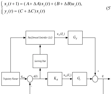
Then, tracking error convergence to zero will occur. One of the properties of the mentioned method is monotonic convergence to zero. Given the above explanation, diagram block in Figure 1 clearly illustrate problem of finding feed-forward control for supercavitating system through d_c. In this figure,K_fb denotes the controller gain whilst Gff and Ge the

feed-forward and feedback time varying transfer function, respectively. Indeed these function are found in terms of

e

d and dc.

3. 3. Systems with Uncertainty One of the properties of this method is that, in spite of system uncertainty, zero convergence is uniformly possible. This is an important advantage over other conventional methods because the possibility of turning sign-definite systems to indefinite ones still exists in the presence of uncertainty. In this section, monotonic convergence is proved with the existence of uncertainty and then zero convergence is discussed. To clarify this point, the following two propositions are first presented:

Proposition 1. Assume the following system with uncertainty:

(57)

( 1) ( ) ( ) ( ) ( ),

( ) ( ) ( )

j j j

j j

x t A A x t B B u t y t C C x t

+ = + D + + D

ìï

í _{= + D}

ïî

( ) fb e

u d

-com

q e t( ) q

fb K

ff G

e G

+

( )

ff c

u d

The closed loop error equation in iterations can be summarized as lumped uncertainty [13].

(58)

1 .

j j

e₊ =H e¢

where H¢ =H + DH and D are matrix of uncertainty coefficients. Also, if DH satisfies the following condition, then, closed loop error will be convergent.

(59) 1

s

D £ <

Proof: Given that a positive part is added to positive statement of ej+1 2 in performance index relation, then

( )

2

1 1

j j

e+ <J a+ . On the other hand, by substituting error relation (58) and learning gain (50) in index (43), the following can be obtained:

( )

2 1 2

1 2

1

2

1 1

1 2

1 ,

,

, j j j j j

j j j j j j

j j j j j

e H P e

J e

w H P e

H P e H P e

e H P e

w H P e

a +

+

+

+ +

+ +

< -+

æ _{D D} ö

ç ÷

+ ç_{ç +} ÷_÷

è ø

(60)

(

)

2

2 2 1

2 1

2 1 2

2 2 1 ,

(1 )

,

j j j

j

j j

j j j

j j

e H P e e

w H P e

e H P e w

w H P e

s

s

+

+

+

+

<

-+

-+

If s<1, then

( )

2 1

j j

J a+ < e ; as a result,

( )

2 2

1 1

j j j

e+ <J a+ < e . In fact, convergent is monotonous. Otherwise, there is no guarantee for convergence. Condition of zero convergence will be investigated in the following proposition.

Proposition 2. According to the previous conditions, in addition to providing monotonic convergence, matrix

j

H P should be sign-definite for zero convergence.

Proof: Consider index relation in (60). Using induction, the following relation can be obtained:

(61)

(

)

2 2

2

2 2 1 2 1

0 2 ₂2

1 ₁

, ,

(1 ) j j j j j j 0

j

j j _{j j}

e H P e e H P e

e e w

w H P e _{w H P e}

s + s +

+ ₊

> - - - >

+ ₊

In other words, index relation is always limited per iteration. One of the necessary conditions for limiting the index in infinite iteration is that the following term should be zero.

(62)

2 1

2 1

,

lim j j j 0 .

j

j j

e H P e

w H P e +

®¥

+

= +

Thus, similar to the previous state, if H Pj is

sign-definite, then this zero convergence will occur. It is enough for the relation to be obtained using Lyapunov

equation in every iteration in order to be sign-definite at the end. Proposition 2 states that uncertainty conditions in the presence of convergence condition in the proposed method are similar to conditions without uncertainty. In other words, by providing conditions of Proposition 1, zero convergence condition will be also provided using the proposed method.

4. SIMULATIONS

In this section, for better efficacy and efficiency of the proposed method, simulation is done. Pitch rate was measured as a supercavitating output and then was used in the feedback loop. The complexity of this system was in its nonlinearity, in which uis constant under supercavitation conditions. Nevertheless, changing pitch rate and attack angle led supercavitation and state matrices to partially change about trim points. So, the system would be time-variant which more complicated its control. Anyway, suppose the desired pitch rate as follows [27]. Here, initial conditions were considered zero. Also, working conditions were considered similar to those in [1]. For the first state, the model with no uncertainty was supposed. Uncertain model was studied in the second case.

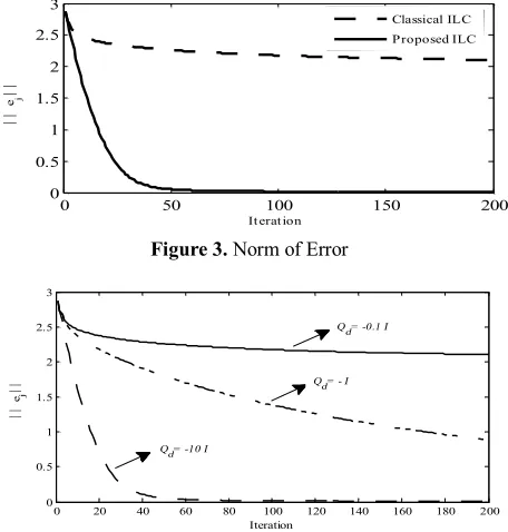
4. 1. Case 1: Perfect Model This case was divided into two parts. The first part showed error improvement trend for different iterations. Figure 2 demonstrates system output for several iterations. Some eigenvalues of matrix H (composed of Markov parameters) were positive and some others were negative. So, this matrix is not sign-definite and norm convergence of closed loop error to zero in iteration using conventional methods was challenging. However, by selecting the proposed method and Qd= -I, monotonic convergence

of error norm to zero can be obtained. Figure 3 indicates error norm for 200 iterations. With more number of iterations, errors were reduced and the system's pitch rate followed the command pitch rate. The second part was related to different values of proposed Q_d for Lyapunov equations. Figure 4 shows the results for different values of proposed Qd. As can be seen in this

figure, the bigger the Qd size, the faster the convergence

Figure 2. Pitch rate Command Tracking for different iteration

Figure 3. Norm of Error

Figure 4. Norm of Error for Different Desired Lyapunov Matrices

Figure 5. Comparison of outcome the proposed ILC in two iterations with respect to the conventional LQR

Figure 6. Norm of the Error

Figure 7. Norm of the Error

As can be seen in this figure, the bigger the Qd, the

faster the convergence to zero would be. For obtaining more convergence, more iteration should be selected. One of the advantages of this method was that it provided one more degree of freedom for designing control necessities, which resulted in bigger Qd for

more convergence without any need to utilize more iteration (in here). Thus, faster convergence would be possible without using more iteration. To show the performance of the proposed technique of modification, the outcome is compared with an optimal LQR method used in [27]. The following figure clarifies preference of the proposed method in comparison with the LQR method.

4. 2. Case 2: System with Uncertainty Consider system (57). There are system's matrix parameters as 10% within nominal value in uncertainty parameters [27]_. Thus, system's uncertainty matrix holds in the following relation:

(63) 0.2 ,

D <

where s =0.2. Figure 6 shows error norm for 100 iterations. As seen in the figure, error norm converged monotonically to zero as iterations increase. But, if

1.2

s= were selected, there would be no guarantee for convergence. Figure 7 clearly illustrates that in 10 iterations. As can be observed in Figure 7, error norm is divergent; in other words, it is not convergent. For this uncertainty bound, there would be no guarantee for convergence. The study is adequate enough for bounded uncertainty, specially for D <1. However, as shown by the unsatisfactory result in Figure 8, for the uncertainty greater than one, there is no guarantee for convergence. Figure 6 is shown to confirm the achievement for provided bound of uncertainty, whereas Figure 7 for the wider uncertainty ( D >1) which is not converging.

5. CONCLUSION

In this article, a new two-state model based on attack angle and pitch rate was presented for more

0 1 2 3 4 5 6 7 8

-30 -20 -10 0 10 20

Time(Sec)

q

(

de

g/

s)

j=5 j=20 j=40 j=100

0 50 100 150 200

0 0.5 1 1.5 2 2.5 3

It erat ion

½

½

ej

½

½

Classical ILC Proposed ILC

0 20 40 60 80 100 120 140 160 180 200 0

0.5 1 1.5 2 2.5 3

Iteration

½½

ej

½½ Qd= - I

Q_d= -0.1 I

Q_d= -10 I

0 0.1 0.2 0.3 0.4 0.5

0 0.5 1 1.5

Time(Sec)

q

(d

eg

/s)

Proposed ILC (k=5) LQR

Proposed ILC (k=10)

0 20 40 60 80 100

0 0.5 1 1.5 2 2.5 3

Iteration

½½

ej

½½

1 2 3 4 5 6 7 8 9 10

2 3 4 5 6 7 8

Iteration

½½

ej

½½

simplification of equations of supercavitating systems for two fin input and cavitator input. The cavitator force could not provide the lift force needed for underwater vehicles; on the other hand, the force produced by the fin was non-minimum phase and slowed the system reaction down. So, for excluding the non-minimum phase part produced by the fin, cavitator feed-forward control was used. For calculating the force needed for the cavitator, iterative learning control was applied. It was also shown that perfect tracking by iterative learning control depended more on the system including supercavitating system.

For this reason, a new model was proposed for solving perfect tracking problem using adaptive compensation matrix in learning gain, and then its calculation in every iteration by solving Lyapunov equation. It was shown that, in the presence of uncertainty in the systems using the new proposed method, monotonic convergence to zero would be possible if uncertainty bound did not exceed the determined value. In Simulation, results verify the tracking of the output to the command trajectory improves with the iterations.

Figure 2 confirms that applying cavitator controller as feed-forward controller increases speed of control reaction with respect to using just the fin angle feedback control. Recently modified ILC converges the norm of tracking error to zero whilst traditional ILC fails to provide zero tracking as depicted in Figure 3. Efficacy of using the proposed method in iterative learning control was shown for calculating feed-forward control for perfect tracking of command pitch rate in the supercavitating system and zero convergence occurred. It was also shown in the simulation that the higher the desired Matrix of the Lyapunov equation, the faster the zero convergence would be. Moreover, in the presence of uncertainty, if uncertainty bound guaranteed the conditions, error norm would tend to zero; otherwise, there would be no guarantee for tracking error norm convergence to zero. Some of the restrictions and relevant improvements are listed here:

- Zero convergence of tracking error may be weakened by existence of measurement noise especially if it is of a random. This effect may be coped with using some filters.

- Misuse of initial condition may cause a problem to achieve zero convergence.

- Basically underwater vehicles under rigid condition are two-dimensional symmetric. The non-minimum phase phenomena of yaw with respect to the fin angle restrict the control reaction and reduce the performance of the system. To overcome this problem, traditional ILC is modified to construct the cavitator control in yaw channel.

]

۱

-۲۷

[

6. REFERENCES

1. Mokhtarzadeh, H., Balas, G. and Arndt, R., "Effect of cavitator on supercavitating vehicle dynamics", Oceanic Engineering,

IEEE Journal of, Vol. 37, No. 2, (2012), 156-165.

2. Vanek, B., Bokor, J., Balas, G.J. and Arndt, R.E., "Longitudinal motion control of a high-speed supercavitation vehicle", Journal

of Vibration and Control, Vol. 13, No. 2, (2007), 159-184.

3. Cao, Z., "Control of supercavitating vehicles based on robust pole allocation methodology", Modern Applied Science, Vol. 5, No. 2, (2011).

4. Tsai, J.S.-H., Chen, F.-M., Yu, T.-Y., Guo, S.-M. and Shieh, L.-S., "Efficient decentralized iterative learning tracker for unknown sampled-data interconnected large-scale state-delay system with closed-loop decoupling property", ISA

Transactions, Vol. 51, No. 1, (2012), 81-94.

5. Tsai, J.S.-H., Du, Y.-Y., Huang, P.-H., Guo, S.-M., Shieh, L.-S. and Chen, Y., "Iterative learning-based decentralized adaptive tracker for large-scale systems: A digital redesign approach",

ISA transactions, Vol. 50, No. 3, (2011), 344-356.

6. Hakvoort, W., Aarts, R.G., van Dijk, J. and Jonker, J., "A computationally efficient algorithm of iterative learning control for discrete-time linear time-varying systems", Automatica, Vol. 45, No. 12, (2009), 2925-2929.

7. Chen, W., Chen, Y.-Q. and Yeh, C.-P., "Robust iterative learning control via continuous sliding-mode technique with validation on an srv02 rotary plant", Mechatronics, Vol. 22, No. 5, (2012), 588-593.

8. Roopaei, M., Shabaninia, F. and Karimaghaee, P., "Iterative sliding mode control", Nonlinear Analysis: Hybrid Systems, Vol. 2, No. 2, (2008), 256-271.

9. Wu, H., Chen, J.-S., Li, M.-F., Durrett, R.P., Chen, W. and Moore, K.L., "Iterative learning control for a fully flexible valve actuation in a test cell", SAE International Journal of

Passenger Cars-Electronic and Electrical Systems, Vol. 5, No.

1, (2012), 55-61.

10. Azevedo-Perdicoúlis, T.-P. and Jank, G., "Disturbance attenuation of linear quadratic ol-nash games on repetitive processes with smoothing on the gas dynamics",

Multidimensional Systems and Signal Processing, Vol. 23, No.

1-2, (2012), 131-153.

11. Hou, Z., Yan, J., Xu, J.-X. and Li, Z., "Modified iterative-learning-control-based ramp metering strategies for freeway traffic control with iteration-dependent factors", Intelligent

Transportation Systems, IEEE Transactions on, Vol. 13, No.

2, (2012), 606-618.

12. Moore, K.L., "Iterative learning control for deterministic systems, Springer, (1993).

13. Yang, S., Qu, Z., Fan, X. and Nian, X., "Novel iterative learning controls for linear discrete-time systems based on a performance index over iterations", Automatica, Vol. 44, No. 5, (2008), 1366-1372.

14. Cai, Z., Freeman, C.T., Lewin, P.L. and Rogers, E., "Iterative learning control for a non-minimum phase plant based on a reference shift algorithm", Control Engineering Practice, Vol. 16, No. 6, (2008), 633-643.

15. Ghosh, J. and Paden, B., "A pseudoinverse-based iterative learning control", Automatic Control, IEEE Transactions on, Vol. 47, No. 5, (2002), 831-837.

16. Owens, D.H. and Chu, B., "Modelling of non-minimum phase effects in discrete-time norm optimal iterative learning control",

International Journal of Control, Vol. 83, No. 10, (2010),

17. Arimoto, S., Kawamura, S. and Miyazaki, F., "Bettering operation of robots by learning", Journal of Robotic systems, Vol. 1, No. 2, (1984), 123-140.

18. Arimoto, S., Kawamura, S. and Miyazaki, F., "Bettering operation of dynamic systems by learning: A new control theory for servomechanism or mechatronics systems", in Decision and Control, 1984. The 23rd IEEE Conference on, Vol. 23, No. Issue, (1984), 1064-1069.

19. Owens, D.H. and Hätönen, J., "Iterative learning control—an optimization paradigm", Annual Reviews in Control, Vol. 29, No. 1, (2005), 57-70.

20. Owens, D., Tomas-Rodriguez, M. and Daley, S., "Limit sets and switching strategies in parameter-optimal iterative learning control", International Journal of Control, Vol. 81, No. 4, (2008), 626-640.

21. Owens, D. and Daley, S., "Iterative learning control— monotonicity and optimization", International Journal of

Applied Mathematics and Computer Science, Vol. 18, No. 3,

(2008), 279-293.

22. Hätönen, J., Owens, D.H. and Feng, K., "Basis functions and parameter optimisation in high-order iterative learning control",

Automatica, Vol. 42, No. 2, (2006), 287-294.

23. Mokhtarzadeh, H., "Supercavitating vehicle modeling and dynamics for control", university of minnesota, (2010), 24. Prestero, T.T.J., "Verification of a six-degree of freedom

simulation model for the remus autonomous underwater vehicle", Massachusetts institute of technology, (2001), 25. Vanek, B., "Control methods for high-speed supercavitating

vehicles, ProQuest, (2008).

26. Xie, L., Ding, J. and Ding, F., "Gradient based iterative solutions for general linear matrix equations", Computers & Mathematics

with Applications, Vol. 58, No. 7, (2009), 1441-1448.

27. Goel, A., "Robust control of supercavitating vehicles in the presence of dynamic and uncertain cavity", University of Florida, (2005),

Perfect Tracking of Supercavitating Non-minimum Phase Vehicles Using a New

Robust and Adaptive Parameter-optimal Iterative Learning Control

M. Yahyazadeh, A. Ranjbar Noei

Faculty of Electrical Engineering, Noshiravani University of Technology, Babol, Iran,

P A P E R I N F O

Paper history: Received 24 June 2013

Received in revised form 29 October 2013 Accepted 07 November 2013

Keywords:

Iterative Learning Control Convergence

Supercavitating Vehicle Model

هﺪﯿﮑﭼ

وﭻﯿﭘخﺮﻧﺐﺴﺣﺮﺑﻪﺘﻟﺎﺣودﺪﯾﺪﺟلﺪﻣسﺎﺳاﺮﺑﯽﻧﻮﯿﺳﺎﺘﯾوﺎﮐﺮﭘﻮﺳﻢﺘﺴﯿﺳﻖﯿﻗدﯽﺑﺎﯾدرياﺮﺑيﺪﯾﺪﺟشور،ﻪﻟﺎﻘﻣﻦﯾارد

ﯽﻣﻪﺋارارﻮﺗﺎﺘﯾوﺎﮐوﮏﻟﺎﺑيدوروودياﺮﺑﻪﻠﻤﺣﻪﯾواز

ددﺮﮔ

.

تاﺮﯿﯿﻐﺗﻪﺑﺖﺒﺴﻧنﻮﯿﺳﺎﺘﯾوﺎﮐﺮﭘﻮﺳﻢﺘﺴﯿﺳﭻﯿﭘخﺮﻧﯽﺟوﺮﺧ

ﻪﯾواز

زﺎﻓﻢﻤﯿﻨﯿﻣﺮﯿﻏ،ﮏﻟﺎﺑ

،ﺖﺳا

نآ ﻦﻤﺿ

ﺲﮑﻋﻪﮐ

ﯽﻣﺪﻨﮐنﺎﻣﺮﻓﭻﯿﭘخﺮﻧلﺮﺘﻨﮐياﺮﺑنآﻞﻤﻌﻟا

ﺪﺷﺎﺑ

.

ﯽﻤﺘﺴﯿﺳﻦﯿﻨﭼلﺮﺘﻨﮐ

ﺲﮑﻋﻪﺑﺖﺒﺴﻧﻢﺘﺴﯿﺳﺦﺳﺎﭘﺖﻋﺮﺳﺶﯾاﺰﻓاوﻦﯿﻌﻣﯽﻧﺎﻣزهزﺎﺑﮏﯾرد

ﺖﺳازﺎﺑﻞﺋﺎﺴﻣءﺰﺟنﺎﻨﭽﻤﻫﮏﻟﺎﺑﯽﻟﺮﺘﻨﮐﻞﻤﻌﻟا

.

ياﺮﺑ

ﯽﻣﻞﮑﺸﻣﻦﯾاﻊﻓر

ﺶﯿﭘلﺮﺘﻨﮐزاناﻮﺗ

زاورﻮﺧ

ﺑﻖﯾﺮﻃ

ﻪ

ﺑرﻮﺗﺎﺘﯾوﺎﮐيﺮﯿﮔرﺎﮐ

ﻪ

ﺶﯿﭘﺮﯿﺴﻣردلﺮﺘﻨﮐناﻮﻨﻋ

دﺮﮐهدﺎﻔﺘﺳا،رﻮﺧ

.

ﺑﻪﻟﺎﻘﻣﻦﯾاهﺪﯾا

ﻪ

ﺑرﻮﺗﺎﺘﯾوﺎﮐيدوروﻖﯿﻗدندروآﺖﺳد

ﻪ

لﺮﺘﻨﮐزاهدﺎﻔﺘﺳاﺎﺑﺖﯿﻌﻄﻗمﺪﻋرﻮﻀﺣردﯽﺑﺎﯾدرﻞﻤﻋدﻮﺒﻬﺑرﻮﻈﻨﻣ

ﺖﺳاهﺪﻧﻮﺷراﺮﮑﺗﺮﯿﮔدﺎﯾ

.

لﺮﺘﻨﮐﺮﺑﯽﻨﺘﺒﻣيﺪﯾﺪﺟشورﻪﻟﺎﻘﻣﻦﯾا،ﻦﯾاﺮﺑهوﻼﻋ

ﺮﺘﻣارﺎﭘهﺪﻧﻮﺷراﺮﮑﺗﺮﯿﮔدﺎﯾ

-ﺑﻪﻨﯿﻬﺑ

ﻪ رﻮﻈﻨﻣ

ﻢﺘﺴﯿﺳﻖﯿﻗدﯽﺑﺎﯾدرﻪﻠﺌﺴﻣﻞﺣ

ﺖﻣﻼﻋﻂﯾاﺮﺷﺪﻗﺎﻓﻪﮐﯽﯾﺎﻫ

-ﯽﻣﻢﺘﺴﯿﺳندﻮﺑﻦﯿﻌﻣ

ﺑﺎﺑ؛ﺪﻨﺷﺎﺑ

ﻪ

ردﻒﻧﺎﭘﺎﯿﻟﯽﻘﯿﺒﻄﺗهﺮﻬﺑيﺮﯿﮔرﺎﮐ

ﯽﻣﻪﺋاراهﺪﻧﻮﺷزوﺮﺑلﺮﺘﻨﮐ

ﺪﯾﺎﻤﻧ

.

ﯽﯾاﺮﮕﻤﻫﻞﮑﺸﻣ،راﺮﮑﺗﺮﺑﯽﻨﺘﺒﻣﻒﻧﺎﭘﺎﯿﻟﻪﻟدﺎﻌﻣﻞﺣزاهدﺎﻔﺘﺳاﺎﺑنآرد

يﺎﻄﺧﻪﺑﺖﺧاﻮﻨﮑﯾ

مﺮﻧمﻮﻬﻔﻣ ﻪﺑﺮﻔﺻ ﯽﺑﺎﯾدر

2

ﯽﻣ ﻊﻔﺗﺮﻣ

ددﺮﮔ

.

ﻪﯿﺒﺷ ﺞﯾﺎﺘﻧ

يزﺎﺳ ،

ﺮﯿﮔدﺎﯾلﺮﺘﻨﮐ ياﺮﺑ ار رﻮﮐﺬﻣ شور ﺮﺛا ﯽﯾارﺎﮐودﺮﮑﻠﻤﻋ

هﺪﻨﻨﮐلﺮﺘﻨﮐﻪﺑﺖﺒﺴﻧهﺪﻧﻮﺷراﺮﮑﺗ

ﯽﻣنﺎﺸﻧ،نﻮﯿﺳﺎﺘﯾوﺎﮐﺮﭘﻮﺳتﺎﺑرياﺮﺑلواﺪﺘﻣيﺎﻫ

ﺪﻫد

.