AN EFFICIENT ALGORITHM TO INTER AND INTRA-CELL
LAYOUT PROBLEMS IN CELLULAR MANUFACTURING
SYSTEMS WITH STOCHASTIC DEMANDS
R. Tavakoli-Moghadam*
Department of Industrial Engineering, Faculty of Engineering Tehran University, P.O. Box 11365/4563, Tehran, Iran, [email protected]
B. Javadi
Department of Industrial Engineering, Mazandaran University of Science and Technology Babol, Iran
F. Jolai and S.M. Mirgorbani
Department of Industrial Engineering, Faculty of Engineering Tehran University, P.O. Box 11365/4563, Tehran, Iran
*Corresponding Author
(Received: January 31, 2005 - Accepted in Revised Form: August 9, 2006)
Abstract In the design of a cellular manufacturing system (CMS), one of the important problems is the CMS layout. This paper presents a new mathematical model concerning inter-cell and intra-cell cost in layout problems in cellular manufacturing systems with stochastic demands. The objective of the model is to minimize the total cost incurred by the inter-cell and intra-cell movements. The proposed model determines the location of each machine in each cell and the location of cells on the shop floor with respect to the confidence level determined by the decision maker. The proposed model is a non-linear model which cannot be easily optimally solved. Thus, a linearization approach is used and the linearized model is then solved by a linear optimization software. Even after linearization, the large-sized problems are still difficult to solve, there fore a Simulated Annealing (SA) method is developed. To verify the quality and efficiency of the SA algorithm, a number of test problems with different sizes are solved and the results are compared with solutions obtained by Lingo 8 in terms of objective function values and computational time.
Key Words Machine/Cellular Layout, Intra/Inter-Cell Movement, CMS, Stochastic Demands, Simulated Annealing
ﻩﺪﻴﻜﭼ
ﻲﻟﻮﻠﺳﺪﻴﻟﻮﺗﻢﺘﺴﻴﺳﻲﺣﺍﺮﻃﺭﺩ (CMS)
ﻞﻳﺎﺴﻣﻦﻳﺮﺘﻤﻬﻣﺯﺍﻲﮑﻳ،
ﻱﺪـﻴﻟﻮﺗﻱﺎـﻫﻝﻮﻠـﺳﻥﺎﻣﺪﻴﭼﻩﻮﺤﻧ
ﺖﺳﺍ
.
ﻪﻨﻳﺰﻫﺎﺑﻪﻄﺑﺍﺭﺭﺩﺪﻳﺪﺟﻲﺿﺎﻳﺭﻝﺪﻣﮏﻳ،ﻪﻟﺎﻘﻣﻦﻳﺍ ﻭﻲﻟﻮﻠﺳﻥﻭﺭﺩﺕﺎﮐﺮﺣﻱﺎﻫ
ﻞﻳﺎﺴـﻣﺭﺩﻲﻟﻮﻠـﺳﻦﻴـﺑ
ﻢﺘﺴﻴﺳﻥﺎﻣﺪﻴﭼ
ﻲﻣﻪﻳﺍﺭﺍﻲﻟﺎﻤﺘﺣﺍﻱﺎﺿﺎﻘﺗﺎﺑﻲﻟﻮﻠﺳﺪﻴﻟﻮﺗﻱﺎﻫ ﻫﺩ
ﺪ
.
ﻤﮐﻝﺪﻣﻑﺪﻫ ﻪﻨﻴ
ﻪﻨﻳﺰﻫﻱﺯﺎﺳ
ﻩﺪﺷﺩﺎﺠﻳﺍﻱﺎﻫ
ﺯﺍ
ﻲﻟﻮﻠﺳﻦﻴﺑﻭﻲﻟﻮﻠﺳﻥﻭﺭﺩﺕﺎﮐﺮﺣ ﺖﺳﺍ
.
ﺭﺍﻝﺪﻣ
ﻪﻳﺍ ﺷ
ﻦﻴﺷﺎﻣﺯﺍﮏﻳﺮﻫﻥﺎﮑﻣ،ﻩﺪ
ﺎﻫ
ﺮـﻫﻥﺎﮑﻣﻭﺎﻫﻝﻮﻠﺳﺭﺩ
ﻝﻮﻠﺳﺯﺍﮏﻳ
ﺑﺍﺭﻩﺎﮔﺭﺎﮐﻒﮐﺭﺩﺎﻫ
ﻥﺎﻨﻴﻤﻃﺍﺢﻄﺳﻪﺑﻪﺟﻮﺗﺎ
ﺺﺨﺸﻣ ﺷ ﺪ
ﻂﺳﻮﺗﻩ ﻩﺪﻧﺮﻴﮔﻢﻴﻤﺼﺗ
ﻲﻣﻦﻴﻌﻣ ﺪـﻳﺎﻤﻧ
.
ﻭﻩﺩﻮﺑﻲﻄﺧﺮﻴﻏﻩﺪﺷﻪﻳﺍﺭﺍﻝﺪﻣ ﻪﻨﻴﻬﺑ
ﺳ ﻥﺁﻱﺯﺎ ﻧﺮﻳﺬﭘﻥﺎﮑﻣﺍﻲﺘﺣﺍﺮﺑ ﺖﺴﻴ
.
ﻦﻳﺍﺮﺑﺎﻨﺑ ﺍﺪﺘﺑﺍ ﻄﺧﺵﻭﺭﮏﻳ ﻱﺯﺎﺳﻲ
ﻪﺘﻓﺮﮔﺭﺎﮑﺑﻥﺁﺩﺭﻮﻣﺭﺩ ﺪﺷ
ﻩ
ﺲﭙﺳﻭ
ﻲﻄﺧﻱﺯﺎﺳﻪﻨﻴﻬﺑﺭﺍﺰﻓﺍﻡﺮﻧﮏﻳﺯﺍﻩﺩﺎﻔﺘﺳﺍﺎﺑ ﻪﻟﺎﺴﻣ
ﻞﺣ ﺖﺳﺍﻩﺪﻳﺩﺮﮔ
.
ﻲﻟﻭ
ﺭﺩﻩﺪﺷﻲﻄﺧﻝﺪﻣﻲﺘﺣﻪﮑﻴﻳﺎﺠﻧﺁﺯﺍ ﻩﺯﺍﺪﻧﺍ
ﻲﮔﺪﻴﭽﻴﭘﻱﺍﺭﺍﺩﻻﺎﺑ ﺖﺳﺍ
، ﻦﻳﺍﺮﺑﺎﻨﺑ
ﻪـﻳﺎﭘﺮﺑﻢﺘﻳﺭﻮﮕﻟﺍﮏﻳ Simulated
Annealing
ﻞﺣﻱﺍﺮﺑ ﺴﻣ
ﺎ ﻪﻟ
ﺪﺷﻩﺩﺍﺩﻪﻌﺳﻮﺗ ﺖﺳﺍﻩ
. ﻢﺘﻳﺭﻮـﮕﻟﺍﻲﻳﺍﺭﺎﮐﻭﺩﺮﮑﻠﻤﻋﺪﻴﻳﺎﺗﻱﺍﺮﺑ SA
ﺭﻮـﺑﺰﻣ
ﻞﻳﺎﺴـﻣ،
ﻲﻧﻮﮔﺎﻧﻮﮔ ﻩﺯﺍﺪﻧﺍﺎﺑ
ﻳﺎﺘﻧﻭﻩﺪﺷﻞﺣﻒﻠﺘﺨﻣﻱﺎﻫ ﺞ
ﻩﺪﻣﺁﺖﺳﺪﺑ ﺏﺍﻮﺟﺎﺑ
ﻱﺎﻫ
ﻞـﺻﺎﺣ
ﻡﺮـﻧﺯﺍ
ﺭﺍﺰـﻓﺍ Lingo 8
ﺎـﺑ
ﻪﺴﻳﺎﻘﻣﻲﺗﺎﺒﺳﺎﺤﻣﻥﺎﻣﺯﻭﻑﺪﻫﻊﺑﺎﺗﺭﺍﺪﻘﻣﻪﺑﻪﺟﻮﺗ ﺷ
ﺪ ﺖﺳﺍﻩ
.
1. INTRODUCTION
Cellular manufacturing (CM) is the application of group technology (GT) in manufacturing systems.
design functions.
The design for cellular manufacturing involves three stages [1] which follow: (1) cell formation by grouping parts into families and machines into cells, (2) creating a layout of the cells within the shop floor (i.e., inter-cell layout); (3) creating a layout of machines within each cell (i.e., intra-cell layout).The realization of benefits expected from cellular manufacturing largely depends on how effectively the three stages of the design have been performed [2].
In the first stage, Tavakkoli-Moghaddam et al. [3] proposed a generalized linear-mixed integer programming approach to simultaneously group machines and part families under a dynamic environment by assuming inter-cell movement, alternative process plan, machine relocation, replicate machines, sequence operation, cell size and machine capacity limitation. Tavakkoli-Moghaddam et al. [4] presented a new mathematical model of a cell formation problem (CFP) for a multi-period planning horizon where the product mix and demand are different in each period. They proposed a memetic algorithm (MA), in which a simulated annealing (SA) is the local search engine, to find the optimal number of cells at each period as well.
The cellular Manufacturing System (CMS) layout problems have not received adequate attention from researchers in comparison to cell formation in the past two decades [5]. For this lack of information on layouts, the benefits of CMS can not be validated [6]. A key element to exploit the benefits of CM is efficient layout designs. A poor physical layout will offset some or all expected benefits. The right solution to plant layout problems is important because material handling costs have been estimated to range from 20% to 50% of the total manufacturing operating expenses. An efficient facility layout can reduce these costs by at least 10% to 30% [7].
There are a number of approaches for layout problems in CMS. Alfa et al. [8] formulated a model for solving only intra-cell layout problems. However, Das [9] formulated a model for solving inter-cell layout problems. Bazargan-Lari et al. [2] presented the application of an integrated approach to the three phases of cellular design manufacturing to White-goods manufacturing company in Australia. Ho and Moodie [10]
addressed a cell layout problem combining a search algorithm and linear programming model to design a cell layout and its flow paths. Salum [6] proposed a two-phase method to design a cell layout that reduces the total manufacturing lead time.
Wang et al [5] formulated a model to solve the facility layout problem in CMS with a deterministic variable demand over the product life cycle. Their objective minimizes the total material handling cost and solves both inter and intra-cell facility layout problems simultaneously. Wu et al. [11] applied a genetic algorithm for cellular manufacturing design and layout. Solimanpur et al. [12] proposed ant colony optimization algorithm to inter-cell layout problems in cellular manufacturing. The performance of the proposed algorithm is compared with other heuristics developed for facility layout problems as well as many other ant algorithms recently developed for the quadratic assignment problem (QAP).
Usually, facility layout studies result from changes that occur in the requirements for space, equipment and people. If requirements change frequently, then it is desirable to plan for the change and to develop a flexible layout that can be modified, expanded, or reduced easily [13]. Flexibility can be achieved by utilizing modular equipment, general-purpose production equipment and material handling devices, etc. The change in the design of and, the processing sequences for existing products, quantities of production and associated schedules, and the structure of organization and/or management philosophies (e.g. centralized, decentralized, hierarchical, etc.) can lead to changes in the layout. When these changes occur frequently, it is important for the layout to accommodate them. Such layouts (called flexible layout) [14] impact on the change of the design of the facility pointed to the need for a facility that can respond to change. An important part of the response to change is the need to rearrange workstations or modify the system structure based on changing functions, volumes, technology, product mix and so on.
determined [15]. With the introduction of new parts and changed demands, new locations for the facilities might be necessary in order to reduce excessive material handling costs (for a detailed discussion on DLP, the reader can refer to [16]). Some authors approached the layout problem with uncertain parameters by generating a stochastic model, Rosenblatt and Lee [17] consider a scenario where contracts of negotiation exist between the producer and the customer, but exact order levels are not clearly defined. Therefore Rosenblatt and Lee [17] proposed, as an alternative, an interesting robust approach to the problem, considering all the scenarios corresponding to different levels of market demand: highest (H) most likely (M) and lowest (L). The above-mentioned authors measure the robustness of an alternative by the number of times that its solution lies within a pre-specified percentage of the optimal solution for every scenario. This approach does not take the limitation in the facility capacity, into account this constraint, in fact, causes some combinations of levels product to overcome the production capacity, and therefore to be unfeasible. Rosenblatt and Kropp [18] studied a stochastic single period for the QAP formulation. Kouvelist et al. [19] also used the QAP model to study single and multi-period layout problems. Norman and Smith [20] introduced a mathematical model of the block layout problem while considering uncertainty in material handling costs on a continuous scale by the use of expected value and standard deviation from product forecast.
For covering the lack of information on CMS layouts, the aim of this paper is to present a new mathematical model for inter and intra-cell layout problems in cellular manufacturing systems with stochastic demands. The objective is to minimize the total costs of inter and intra-cell movements in both machine and cell layout problems simultaneously.
The novelty of the proposed model is arranging machines within each cell as well as cells within the shop floor with respect to the confidence level determined by the decision maker.
This paper is organized as follows: the problem formulation is described in Section 2. In Section 3 the simulated annealing (SA) algorithm has been used and designed to solve the proposed model.
The computational results are reported in Section 4 and the conclusion is given in Section 5.
2. PROBLEM FORMULATION
In this section, we formulate the nonlinear mathematical model for both dynamic machine (i.e., intra-cell) and cell (i.e., inter-cell) layout problems with stochastic demands in cellular manufacturing systems. This proposed model deals with the minimization of the integrated (intra-cell and inter-cell) cost function. The machine layout problem seek to find the optimal arrangement of machines within each cell as well as cells within the shop floor. This model can be considered as a bi-quadratic assignment problem.
2.1. Assumptions of the Model The assumptions are described as follows:
1- Cell formation is first completed and known as a prior, i.e. which machines belong to which cells.
2- Part demands are independent with the normal probability distribution.
3- Parts are moved in batches between/inside cells.
4- Inter/intra cell batch sizes are constant for all productions.
5- The money time value is not considered. 6- Shapes and dimensions of the shop floor are
not restricted.
7- Equal-sized machines or cells are considered.
8- Each cell is laid out in a U-shape. The length and width of which are is known. Besides, material handling flows along the U-shape. 2.2.The Mathematical Model To build the model, the following symbols are used.
2.2.1. Indices
i, j index for machines ( i, j= 1,…, M ), i # j c, l index for cells ( c, l = 1,…, C ), c # l
p, q index for machine locations ( p, q=1,…, M ),
p # q
2.2.2. Input Symbols
K number of part types.
M number of machine locations.
C number of cell locations.
Dk demand for part k for a given planning
horizon.
Bk transfer batch size for part k. COk cost of trips part k.
Nki operation number for the operation done on
part k by machine i.
dpq distance between machine locations p , q. dtu distance between cell locations t, u.
aic equal to 1, if machine type i assign to cell c, 0, otherwise.
ZP standard normal Z for percentile P.
E( ) expected value. Var( ) variance value
2.2.3. Decision Variables
Xiph equal to 1, if machine i is in location
machine 0, otherwise:
Xcth equal to 1, if cell c is in location cell t 0,
otherwise.
2.2.4. The Mathematical Model
The nonlinear mathematical formulation for the facility layout problem in cellular manufacturing systems is presented below:cell inter cell intra
minz= +
∑ = ∑= ∑= ⎟ ⎟ ⎠ ⎞ ⎜ ⎜ ⎝ ⎛ ∑ = ∑= ⎟ ⎠ ⎞ ⎜ ⎝ ⎛ + ∑ = ∑= ∑= ∑= ∑= = C c M 1 i M j M p M q jq X ip X pq d ijc F P Z jq X C c M i M j M p M q ip X pq d ijc F 1 1 2 1 1 Var
1 1 1 1 1
) ( E cell intra jc a ic a ij F ijc
F )=E( )× × (
E
∑ = = K
k fijk ij
F
1E ( )
) ( E ⎪ ⎪ ⎩ ⎪⎪ ⎨ ⎧ = − × = otherwise. 0 1, if ) ( E ) (
E Bk COk Nki N kj k D ijk f 2 2 ) ( Var ) (
Var Fijc = Fij ×aic × a jc
∑ = = K
k fijk
ij F
1Var ( ) ) ( Var ⎪ ⎪ ⎩ ⎪⎪ ⎨ ⎧ = − × = otherwise. 0 1, if 2 2 ) ( Var ) (
Var Bk COk Nki Nkj k D ijk f ∑ = ∑= ⎟ ⎟ ⎠ ⎞ ⎜ ⎜ ⎝ ⎛ ∑ = ∑= + ∑ = ∑= ∑= ∑= = C c C l C t lu X ct X C u tu d cl F P Z lu X ct X C c C l C t C u tu d 1 1 2 1 1 ) ( Var
1 1 1 1
) cl F ( E cell inter s.t. ∑ = = ∀ M
i 1xip 1 p (2)
∑
= = ∀
M
p 1xip 1 i
(3) ∑ = = ∀ C c t ct x 1
1 (4)
∑
= = ∀
C
t 1xct 1 c
(5)
{ }
0,1 and integer ∈ ct x , lu x , jq x , ipx (6)
The objective function (1) consists of two terms: The first term (1.1) is equal to the intra-cell movement cost. In this Equation, Fijc shows the
number of trips made by the equipment which handles the material between machines i and j
within cell c. The second term (1.2) is equal to the inter-cell movement cost. In this Equation Fcl shows the number of trips made by the equipment which handles the material between cells c and l.
2.2.5. Linearization of the Mathematical
Model
It is obvious that Equations 1.1 and 1.2 are nonlinear functions. In fact, these functions can be linearized in two stages. In the first stage, define new binary integer variables Xijpq and Xcltu, whichare computed by the following Equations:
jq X ip X ijpq
X = ∀i,j,p,q
lu X ct X cltu
X = ∀c,l,t,u
By considering the above Equations, the following should also be added to the proposed model by enforcing these four linear inequalities simultaneously: 0 1.5≥ + − −xip xjq ijpq
X (7)
0
1.5Xijpq−xip−xjq ≤ (8)
0 1.5≥ + − −Xct Xlu cltu
X (9)
0
1.5 Xcltu−Xct−Xlu≤ (10)
In the second stage, we define new integer variables Yij and Wcl:
ij Y ijpq X M p M q pq d = ∑ =1 ∑=1
∀i,j (11)
cl W cltu X C t C
u dtu
= ∑
=1 ∑=1 c,l
∀ (12)
Naslund’s approximations [21] to linearize such nonlinear functions are to substitute Equations 1.1 and 1.2 into the following two inequalities:
(1.1) Intra cell
⎢ ⎢ ⎢ ⎢ ⎢ ⎣ ⎡ ⎪⎭ ⎪ ⎬ ⎫ ⎪⎩ ⎪ ⎨ ⎧ ∑ = ∑= ∑= + ∑ = ∑= ∑= 2 1
1 1 1
) ( VAR )
1 1 1
( E C c M i M j ijc F P Z ij Y C c M i M j ijc F ⎢ ⎢ ⎢ ⎣ ⎡ ⎪⎭ ⎪ ⎬ ⎫ ⎪⎩ ⎪ ⎨ ⎧ ∑ = ∑= ∑= ∑ = ∑= ∑= ⎩⎨ ⎧ ⎟ ⎠ ⎞ ⎜ ⎝ ⎛ − − 2 1
1 1 1
) ( VAR 1 1 1
1 C c M i M j ijc F C c M a M b ab Y ⎥ ⎥ ⎥ ⎥ ⎥ ⎦ ⎤ ⎪ ⎪ ⎭ ⎪ ⎪ ⎬ ⎫ ⎥ ⎥ ⎥ ⎥ ⎥ ⎦ ⎤ ⎟⎟ ⎟ ⎠ ⎞ ⎜⎜ ⎜ ⎝ ⎛ − ⎟ ⎟ ⎠ ⎞ ⎜ ⎜ ⎝ ⎛ ∑ = ∑= ∑= − 2 1 ) ( VAR
1 1 1VAR( ) Fabc
C
c M
i M
j Fijc
(1.2) Inter cell
⎥ ⎥ ⎥ ⎥ ⎦ ⎤ ⎪ ⎪ ⎭ ⎪⎪ ⎬ ⎫ ⎥ ⎥ ⎥ ⎦ ⎤ ⎟ ⎟ ⎠ ⎞ − ⎜ ⎜ ⎝ ⎛ ⎟ ⎟ ⎠ ⎞ ⎜ ⎜ ⎝ ⎛ ∑ = ∑= − ∑ = ∑= ⎪⎩ ⎪ ⎨ ⎧ ⎢ ⎢ ⎣ ⎡ ⎪⎭ ⎪ ⎬ ⎫ ⎪⎩ ⎪ ⎨ ⎧ ∑ = ∑= ⎟ ⎠ ⎞ ⎜ ⎝ ⎛ − − ⎢ ⎢ ⎢ ⎢ ⎣ ⎡ ⎪⎭ ⎪ ⎬ ⎫ ⎪⎩ ⎪ ⎨ ⎧ ∑ = ∑= + ∑ = ∑= 2 1 ) ( Var 1 1 ) ( Var 2 1
1 1 1 1
) ( Var 1 2 1 1 1 ) VAR( ) 1 1 ( E eo F C c C l cl F C e C o C c C l cl F eo W C c C l cl F p Z cl W C c C l cl F
3. THE PROPOSED ALGORITHM The proposed model falls in a class of NP-Hard problems. In another words, to find a final optimum solution under these conditions and constraints becomes difficult or even impossible in action or in a reasonable amount of computational time. In this paper, SA algorithm has been used and designed to solve the proposed model.
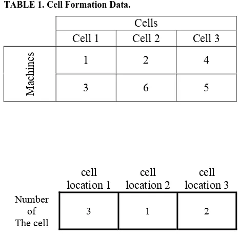
TABLE 1. Cell Formation Data. Cells
Cell 1 Cell 2 Cell 3
1 2 4
Machines 3 6 5
cell location 1
cell location 2
cell location 3
Number of
The cell 3 1 2
Figure 1. A representation of the cells location. algorithmic feature of simulated annealing is that it
provides a means to escape local optima by allowing hill-climbing moves (i.e., moves which worsen the objective function value). SA begins with an initial solution (init_sol) and an initial temperature (T), and an iteration number (E1).
Temperature (T) controls the possibility of the acceptance of a deteriorating solution, and an iteration number (E1) decides the number of
repetitions until it reaches a stable state under the necessarg temperature. Temperature provides a means of flexibility while at high temperatures (early in the search), there is some flexibility to the situation to deteriorate; but at lower temperatures (later in the search) less flexibility exists.
A new neighborhood solution (Φ′) is generated based on T and E1 through a heuristic perturbation
on the existing solutions. The neighborhood solution (Φ′) becomes the current solution (Φ) if the change of an objective function (ΔTC=TC(Φ′)−TC(Φ)
)
is improved (i.e.TC(Φ′) ≤ TC(Φ)). Even though it is not improved, the neighborhood solution becomes a new solution with an appropriate probability basedon )
Δ
(
e T
TC
.
This lowers the possibility of being trapped in a local optimum. The algorithm terminates upon reaching a predetermined temperature (Tc) or if there is no improvement in the objective function after repetition.
3.1.1. Solution representation
Suppose ahypothetical problem in which there are 3 cells and 6 machines. Each of the cells is located in one of the 3 cell locations and each of the machines is in one of the 6 machine locations related. (The number of call locations and machine locations in each cell is respectively equal to the total number of cells and machines).
As we have assumed, cell formation is performed beforehand, so the allocation of machines to cells are known.
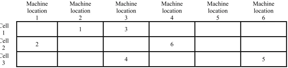
Table 1 displays information about cell formation. A possible representation of the problem can be shown by forming a 3 × 6 array to illustrate the location of each machine in machine locations of their respective cell as is shown in Figure 2.
To represent the assignment of cells to cell location, a 1 × 3 array is formed. Each permutation
of the numbers from 1 to 3 is a possible assignment of the cells to cell locations. Figure 1 shows a sample single row array for the assumed problem: According to Figure 1, cell location 1 is assigned to cell 3, Cell location 2 is assigned to cell 1 and cell location 3 is assigned to cell 2.
3.1.2. Proposed SA algorithm
In this paper, a meta-heuristic algorithm based on simulated annealing (SA) [22] is proposed. The pseudo code of this algorithm is illustrated in Figure 3. The main steps of the proposed SA are as follows: Step 1. Initial solution generationThe initial Solution is randomly generated. For this purpose, as mentioned in secretion 3.1.1, a multi-row, multi-column array is formed and each machine is located randomly in one of the machine locations of its respective cell. Moreover, a random permutation of the numbers of the cells is used as the initial location of the cells in cell locations according to what was described in section 3.1.1.In addition, Initial temperature, Tf, frozen
temperature, Tc, epoch length, E1, the number of
Machine location
1
Machine location
2
Machine location
3
Machine location
4
Machine location
5
Machine location
6 Cell
1 1 3
Cell
2 2 6
Cell
3 4 5
Figure 2. A representation of the machines location.
objective function of the initial solution will be calculated.
Step 2. Temperature updating
The temperature is decreased according to the following Equation:
i T
β
1 i
T + = ×
where, β is the cooling rate and is equal to 0.95. If the updated temperature is not less than frozen temperature, Tc, go to Step 3, otherwise go to Step
6, set counter = 1.
Step 3. Neighborhood generation
In order to obtain the neighborhood solution from the current solution, a cell is randomly chosen, and then a swapping between two machines or a vacant location and a machine in that cell will be performed randomly. In addition two of the available cells are also swapped in the single-row array relating the location of the cells. Step 4. Acceptance criteria
In this step, we decide whether to replace the current solution with the neighborhood solution or not. The current solution will be replaced with the neighborhood solution if its related cost (TC(Φ′)) is less than or equal to the cost of the current solution (TC(Φ)). Even if the neighborhood solution is not better than the current solution, in order to allow the algorithm to leave a local optimum, the neighborhood solution will be accepted if the Metropolis Condition is met. According to Metropolis condition, a worst solution will be accepted as the current solution with the probability of )
Δ
( e )
( Ti
TC A
r P
−
= where
) ( ) (
ΔTC =TC Φ′ −TC Φ .
Step 5. Counter updating
The counter counts the maximum number of solutions generated in each temperature. In this step it is decided whether we have reached the maximum number of solutions in each iteration or not. If the limit is not met (i.e. counter < E1) go to
Begin
Initialize (init_sol, T) Φ=Φ∗=sol
Repeat
For i = 1 to El
Φ′=PERTURB(Φ)
ΔTC = TC(Φ′)−TC(Φ)
if (TC(Φ′) < (TC(Φ) or )>
Δ
(
e T
TC
u~ (0, 1) then Φ=Φ′
if (TC(Φ) < (TC∗(Φ) then Φ∗ =Φ end for
UPDATE (T) Until (Stop-Criterion) End,
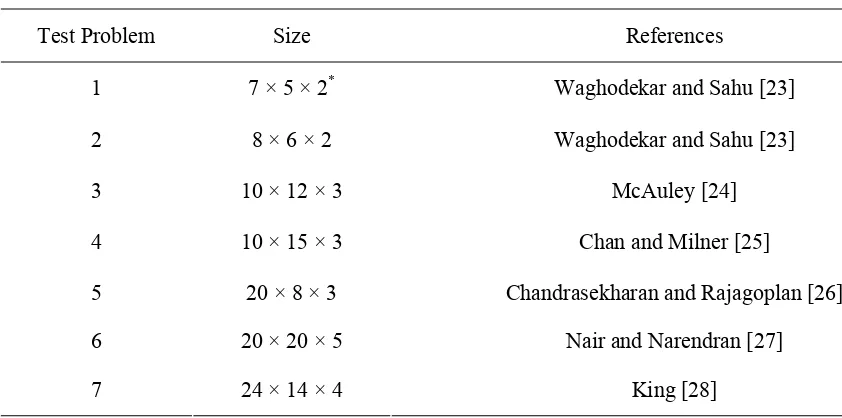
TABLE 2. Sources of Problems.
Test Problem Size References
1 7 × 5 × 2* Waghodekar and Sahu [23]
2 8 × 6 × 2 Waghodekar and Sahu [23]
3 10 × 12 × 3 McAuley [24]
4 10 × 15 × 3 Chan and Milner [25]
5 20 × 8 × 3 Chandrasekharan and Rajagoplan [26]
6 20 × 20 × 5 Nair and Narendran [27]
7 24 × 14 × 4 King [28]
*7 × 5 × 2 ( No. parts × No. machines × No. cells ). Step 4, otherwise, go to Step 2.
Step 6. Termination
The algorithm will be terminated if the current temperature reaches a predetermined temperature of (Tc). Please note that to prevent losing an
optimal solution, the best solution found so far (Φ∗) is kept. A better solution generated from the current solution will be compared with Φ∗and if
better than Φ∗, Φ∗ will be replaced. In the initializing step, Φ∗ is initialized and will be the same as the random initial solution.
4. COMPUTATIONAL RESULTS
The performance of the proposed simulated annealing algorithm (SA) is compared with the Lingo software. This algorithm is coded into the visual basic 6 and run on a Pentium 4, processor at 3 GHz and Windows XP using 512 MB of RAM. To validate and verify the proposed model, six sets of data (problems) have been chosen from the literature (given in Table 2) and then these problems are solved with respect to the different
values of the confidence level. However, we tune other parameter sets as shown below:
E (D) = (1000, 3000) Var (D) = (500-700) Batch size = 10 Cost of trips = 2
Distance between machines = U~ (1, 5) Distance between cells = U~ (5, 30)
We also consider the following SA algorithm assumptions:
(a) Initial temperature 3000 (b) Frozen temperature 10 (c) Cooling rate 0.95 (d) Maximum number of solutions
for each temperature: C×M×P where, C is the number of cells, M is the number of machines and
P is the number of parts.
TABLE 3. Computational Results of 7× 5 ×2 Problem with Different Confidence Levels.
Confidence
Level inter-cell layout intra-cell layout Cost Values
intra-cell inter-cell OFV
cell 2 : 3 - 1 0.6 Cells : 2 - 1
cell 1: 5 - 2 - 4
6194.41 10156.18 16350.59
cell 2 : 1 - 3 0.7 Cells : 2 - 1
cell 1: 5 - 2 - 4
6209.37 10193.74 16403.11
cell 2 : 3 - 1 0.8 Cells : 2 - 1
cell 1: 5 - 2 - 4
6227.10 10238.27 16465.37
cell 2 : 3 - 1 0.9 Cells : 2 - 1
cell 1: 2 - 5 - 4
6251.49 10299.49 16550.98
CPU Time: 00:00:13 Number of variables: 805 and Number of constraints: 857.
TABLE 4. Computational Results of 8× 6 ×2 Problem with Different Confidence Levels.
Confidence
Level inter-cell layout intra-cell layout Cost Values
intra-cell inter-cell OFV
cell 2 : 3 - 1 - 6 0.6 Cells : 2 - 1
cell 1: 5 - 2 - 4
8066.36 22059.90 30126.26
cell 2 : 3 - 1 - 6 0.7 Cells : 2 - 1
cell 1: 5 - 2 - 4
8093.73 22122.11 30215.84
cell 2 : 1 - 3 - 6 0.8 Cells : 2 - 1
cell 1: 2 - 5 - 4
8126.18 22195.83 30322.01
cell 2 : 3 - 1 - 6 0.9 Cells : 2 - 1
cell 1: 2 - 5 - 4
8170.78 22297.19 30466.98
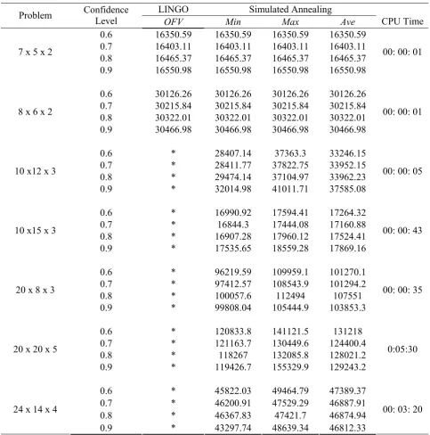
TABLE 5. Computational Results Obtained from Optimal Solution and SA.
LINGO Simulated Annealing
Problem Confidence Level
OFV Min Max Ave CPU Time
0.6 16350.59 16350.59 16350.59 16350.59
0.7 16403.11 16403.11 16403.11 16403.11
0.8 16465.37 16465.37 16465.37 16465.37
7 x 5 x 2
0.9 16550.98 16550.98 16550.98 16550.98
00: 00: 01
0.6 30126.26 30126.26 30126.26 30126.26
0.7 30215.84 30215.84 30215.84 30215.84
0.8 30322.01 30322.01 30322.01 30322.01
8 x 6 x 2
0.9 30466.98 30466.98 30466.98 30466.98
00: 00: 01
0.6 * 28407.14 37363.3 33246.15
0.7 * 28411.77 37822.75 33952.15
0.8 * 29474.14 37104.97 33962.23
10 x12 x 3
0.9 * 32014.98 41011.71 37585.08
00: 00: 05
0.6 * 16990.92 17594.41 17264.32
0.7 * 16844.3 17444.08 17160.88
0.8 * 16907.28 17960.12 17524.41
10 x15 x 3
0.9 * 17535.65 18559.28 17869.16
00: 00: 43
0.6 * 96219.59 109959.1 101270.1
0.7 * 97412.57 108543.9 101294.2
0.8 * 100057.6 112494 107551
20 x 8 x 3
0.9 * 99808.04 105444.9 103853.3
00: 00: 35
0.6 * 120833.8 141121.5 131218
0.7 * 121163.7 130449.6 124400.4
0.8 * 118267 132085.8 128021.2
20 x 20 x 5
0.9 * 119426.7 155329.9 129243.2
0:05:30
0.6 * 45822.03 49464.79 47389.37
0.7 * 46200.91 47529.29 46887.91
0.8 * 46367.83 47421.7 46874.94
24 x 14 x 4
0.9 * 43297.74 48639.34 46812.33
00: 03: 20
* denotes that lingo cannot solve the problem.
can effect inter and intra-cell layouts and corresponding costs. The computational results shown in Table 5 reveal that the proposed SA has the ability to compete the Lingo from a quality
point of view.
solution of the five runs in different confidence levels is the same as the optimal solution solved by the Lingo software. This result reveals that the SA algorithm has the ability to find the optimal solution. That is clearly true for large-sized problems in which the Lingo software cannot produce any results.
6. CONCLUSION
In this paper, a new nonlinear mathematical model is proposed for inter and intra-cell layout problems in cellular manufacturing systems with stochastic demands. The proposed model determines the optimal inter and intra-cell layouts for each confidence level with the aim of minimizing the total costs of inter and intra-cell movements simultaneously.
We solved typical examples in small and large-sized problems under different values of confidence levels and showed how confidence levels can effect the terms of objective function and the inter and intra-cell layouts.
An approximate approach is used to linearize the above nonlinear model. Since even after linearization, the conventional and traditional optimization methods cannot be used for the large-sized problems in reasonable time. Hence, a meta-heuristic efficient algorithm known as simulated annealing (SA) is used and designed to solve the mathematical model.
In the end, different-sized problems involving number of parts, number of machines and number of cells for each confidence level are tested and solved. This is done to show the efficiency of the proposed algorithm. The formulated mathematical model is still open for considering other issues such as cells/machines dimensions, aisles, closeness relationships, and unrestricted locations.
7. REFERENCES
1. Sing, N., “Design of cellular manufacturing systems: an invited review”, European Journal of Operation
Research, Vol. 69, (1993), 284-291.
2. Bazargan-Lari, M., Kaebernick, M. and Harraf, H., “Cell formation and layout design in a cellular manufacturing”,
International Journal of Production Research, Vol. 38,
(2000), 1689-1709.
3. Tavakkoli-Moghaddam, R., Aryanezhad, M. B., Safaei, N. and Azaron, A., “Solving a dynamic cell formation problem using meta-heuristics”, Applied Mathematics
and Computation, Vol. 170, No. 2, (2005), 761-780.
4. Tavakkoli-Moghaddam, R., Safaei, N. and Babakhani, M., “Solving a dynamic cell formation problem with machine cost and alternative process plan by memetic algorithms”,Lecture Notes in Computer Science, Vol. 3777, (2005), 213-227.
5. Wang, T. Y., B. Wu, K. and Liu, Y. W., “A simulated annealing algorithm for facility layout problems under variable demand in cellular manufacturing systems”,
Computers in Industry, Vol. 46, (2001), 181-188.
6. Salum, L., “The cellular manufacturing layout problem”,
International Journal of Production Research, Vol. 38,
(2000), 1053-1069.
7. Tompkins, J. A. and White, J.A., “Facilities Planning”, New York, Wiley, (1984).
8. Alfa, A.S.; Chen, M. and Heragu, S. S., “Integrating the grouping and layout problems in cellular manufacturing systems”, Computers and Industrial Engineering, Vol.
23, (1992), 55-58.
9. Das, S. K., “A facility layout method for flexible manufacturing systems”, International Journal of
Production Research, Vol. 31, (1993), 279-297.
10. Ho, Y. C. and Moodie, C. L., “A hybrid approach for concurrent layout design of cells and their flow paths in a tree configuration”, International Journal of
Production Research, Vol. 38, (2000), 895-928.
11. Wu, X., Chu, C.H., Wang, Y. and Yan, W., “A genetic Algorithm for cellular manufacturing design and layout”,
European Journal of Operational Research, Article in
Press, (2006).
12. Solimanpur, M., Vrat, M. and Shankar, R., “Ant colony optimization alghorithm to the inter-cell layout problem in cellular manufacturing“, European Journal of
Operational Research, Vol. 157, (2004), 592-606.
13. Tompkins, J. A White, J. A., Bozer, Y. A., Frazelle, E. H., Tanchoco, J. M. A. and Trevino, J., “Facilities planning”, New York, Wiley, (1996), 137–285.
14. Abedzadeh, M. and Brien, C., “The potential for virtual cells in a rapid reconfigurable environment”,
Proceedings of the First International Conference on
Industrial Engineering Applications and Practice,
Texas, USA, (1996).
15. Discol, J. and Sawyer, J. H. F., “A computer model for investigating the relayout of batch production areas”,
International Journal of Production Research, Vol. 23,
(1985), 783-794.
16. Balakrishnan, J. and Cheng, C. H., “Dynamic layout algorithms: a state-of-the-art survey”, International
Journal of Management Science, Vol. 26, (1998),
507-521.
17. Rosenblatt, M. J. and Lee, H., “A robustness approach to facilities design”, International Journal of Production
Research, Vol. 25, (1987), 479-486.
19. Kouvelis, P., Kurawarwala, A. A. and Gutierrez, G. J., “Algorithms for robust single and Multiple period layout planning for manufacturing systems”, European
Journal of Operation Research, Vol. 63, (1992),
287-303.
20. Norman, B. A. and Smith, A. E., “A continuous approach to considering uncertainty in facility design”, Computers and Operations Research, Vol. 33, (2006), 1760-1775.
21. Olson, D. L. and Swenseth, S. R., “A linear approximation for chance-constrained programming”,
Journal of Operation Research Society, Vol. 38, (1987),
261-267.
22. Kirkpatrick, S., Gelatt, C. D. and Vecchi, M. P., “Optimization by simulated annealing”, Science, Vol.
220, (1983), 671-680.
23. Waghodekar, P. H. and Sahu, S., “Machine-component cell formation in GT: MACE”, International Journal of
Production Research, Vol. 22, No. 6, (1984), 937–948.
24. McAuley, J., “Machine grouping for efficient production”, Production Engineer, Vol. 51, No. 2, (1972), 53–57.
25. Chan, H. and Milner, D., “Direct clustering algorithm for group formation in cellular manufacturing”, Journal of
Manufacturing Systems, Vol. 1, No. 1, (1982), 65–67.
26. Chandrasekharan, M. P. and Rajagopalan, R., “MODROC: an extension of rank order clustering for group technology”, International Journal of Production
Research, Vol. 24, No. 5, (1986), 1221–1233.
27. Nair, G. J. and Narendran, T. T., “A clustering algorithm for cell formation with sequence data”, International
Journal of Production Research, Vol. 36, No. 1, (1998),
157-179.
28. King, J. R., “Machine-component grouping in production flow analysis: an approach using a rank order clustering algorithm”, International Journal of
Production Research, Vol. 18, No. 2, (1980), 213–