Optimum Shape Design of a Radiant Oven by the Conjugate Gradient Method and a Grid Regularization Approach

International Journal of Engineering

J o u r n a l H o m e p a g e : w w w . i j e . i r

Optimum Shape Design of a Radiant Oven by the Conjugate Gradient Method and a

Grid Regularization Approach

M. Jahanbakhsh Rostamia,_{, S.M. Hosseini Sarvari}b*_{, A. Behzadmehr}a

a

Mechanical Engineering Department, The University of Sistan & Baluchestan, 98135-161, Zahedan, Iran

b

Mechanical EngineeringDepartment, Shahid Bahonar University of Kerman,76175-133, Kerman, Iran

A R T I C L E I N F O

Article history:

Received 9June2011

Accepted in revised form 17May2012

Keywords:

Inverse Geometry Design Radiation

Optimization

A B S T R A C T

This study presents an optimization problem for shape design of a 2-D radiant enclosure with transparent medium and gray-diffuse surfaces. The aim of the design problem is to find the optimum geometry of a radiant enclosure from the knowledge of temperature and heat flux over some parts of boundary surface, namely the design surface. The solution of radiative heat transfer is based on the net radiation method,where the configuration factors are obtained by the Hottel’s crossed-string approach by treating blockage and convex surfaces. The conjugate gradient method is used for minimization of an objective function, which is expressed as the sum of square residuals between estimated and desired heat fluxes over the design surface, and the sensitivity coefficients are calculated by the finite difference method. A regularization approach is proposed to numerically regularize the ill-ordered grids, which are commonly found during the iterative optimization process. Some example problems are presented to show the performance and accuracy of the method. The results show that the optimization procedure can successfully generate the optimum geometry of radiant enclosure.

doi:10.5829/idosi.ije.2012.25.02c.10

1. INTRODUCTION1

Optimum design of radiant enclosures has gained considerable interest in semi conductor and food industries. The main goal of the design problem is to satisfy the uniform heat flux and temperature distributions over the surface of product, namely the design surface. This goal may be attained by regularization of the strengths or the locations of heat sources over the heater surface [1-4]. However, when setting a number of heaters with variable strengths or locations over the heater surface is difficult, expensive or non-practical, optimization of enclosure shape design may be the final solution. The shape optimization may also be combined with other optimization problems in order to achieve the best solution.

In recent years, shape optimization problems have received much attention in a number of engineering applications. Practical applications are found from the optimization of mechanical structures [5-7] to aerodynamic design [8, 9]. In the field of heat transfer,

*_{Corresponding author: Email-[email protected]}

many efforts have been made to optimize the design of fin profiles to produce the maximum heat loss for a specified fin volume. Malekzadeh et al. [10, 11] used a combination of the differential quadrature element method and the golden section search method for maximizing the heat dissipation for any given fin volume with combined convective–radiative heat transfer. Kundu and Das [12] developed a generalized methodology for the optimum design of longitudinal fins, pin fins, and radial fins with uniform volumetric heat generation using the variational method.

by improving the location of a number of control points

representing the B-spline curve of the radiant oven to

achieve the desired goal. Because the GA searches from a population of points, the probability of the search getting trapped in a local minimum is limited. However, the large size of the population makes it very poor in terms of convergence performance so that the iterative procedure, even for micro genetic algorithm which uses a population of five chromosomes, is time consuming. Another tool for optimization of thermal systems is the gradient-based methods such as the Newton method or the conjugate gradient method (CGM) [17]. The main drawback of gradient-based methods is that the result depends on the initial guess. If there is more than one local optimum in the problem, the result will depend on the choice of the starting point, and a global optimum cannot be guaranteed. Another drawback of gradient-based methods is that they depend on the existence of derivatives. For cases where the derivatives of the known parameter with respect to the unknown variables can be found in a straightforward manner, these methods have a good performance, but in most cases it is difficult or extremely expensive to calculate these derivatives precisely. In spite of the above-mentioned drawbacks, the gradient-based methods are more

efficient in convergence rate. This advantage

compensates the drawbacks of the gradient-based methods, and hence even today these methods are widely used for inverse design of complex systems. For example Daun et al. [18, 19] used the gradient based optimization methods for geometry design of a radiant oven through the optimization of locations of a few

control points for the B-spline curves representing the

geometry. Lan et al. [20] reported an approach combining the curvilinear grid generation and conjugate gradient methods for shape design of heat conduction problems. They proposed a redistribution approach to regularize the ill-ordered grids which are commonly generated during the iterative optimization procedure. In the present work, we attempt to find the optimum geometry of a radiant oven to produce the uniform thermal conditions over the design surface. A uniform heat flux is maintained over the heater surface, and the design surface is considered to be isothermal. Then, the aim of the design problem is to produce uniform heat flux distribution over the design surface through optimizing the profile of an adiabatic wall. The radiation transfer equation is solved by the net radiation method and the conjugate gradient method is used to optimize the locations of the nodal points which represent the profile of the adiabatic wall. An efficient regularization approach is used to remove the ill-ordered points which are generated during the iterative procedure and replacing them with new points in alignment. The performance of the optimization method is examined by some numerical experiments and the effects of the initial guess are discussed.

2. DESCRIPTION OF PROBLEM

Figure 1 shows a schematic shape of a radiant enclosure. The design surface is placed horizontally,

and the heater surface has a deviation angle



with the

design surface. The nodal points shown in Figure 1 by

)

,

(

m m

m

x

y

z

are the dynamic nodal points that represent

the shape of the adiabatic wall. Both the design surface and the heater surface are diffuse-black, and the medium is transparent. A uniform heat input is maintained over the entire heater surface. The aim of the design problem is to optimize the geometry of the adiabatic wall by optimizing the locations of dynamic nodal points to produce a uniform heat flux distribution over the temperature-specified design surface.

Figure 1.Schematic shape of the radiant oven and dynamic nodal points at the adiabatic surface

3. DIRECT PROBLEM

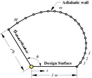
Consider a radiant enclosure with K discrete internal

surfaces as shown in Figure 2a. The objective is to analyze the radiation exchange between the surfaces involving two types of boundary conditions; the surfaces with specified emissive power and the surfaces with specified heat flux.

The net radiation method is used to solve the radiation exchange in the radiant enclosure. In this method, the boundary is subdivided into surface elements. The equation of radiation exchange for surface elements with specified emissive power can be described by the following equation:









, 1

1

1 ,

1 F Jj kEbk k K

K

j

j k k

kj    



 

 

 (1a)

whereas,the radiative transfer equation for other surface

elements with specified heat flux is given by [21]:



F



J q K k K

K

j

k j j k

kj     





 , 1 1

1

 (1b)

where



_kj is the Kronicker delta defined by:

  

  

j k

j k

kj

0 1

 (2)

1 2

3 m

M



x 1 m

1 m

Design Surface

H ea

te_r S

ur_fa ce

here,

J

,

q

and

E

_b denote the radiosity, heat flux and the emissive power, respectively. The set of Eq. (1) is solved to calculate the outgoing heat fluxes,

K j

t

Jj(), 1,, , then the unknown boundary condition

(emissive power or heat flux) is determined by the following equation:

K k E

J

qk k bk

k

k    

 1 , 1 ,   (3) (a) (b)

Figure 2.(a) Schematic shape of a radiant enclosure and (b) parameters in the Hottel’s crossed-string method

The configuration factors are calculated by the Hottel’s crossed-string method (see Figure 2b).

k bc ad bd ac j k A A A A A F 2      (4)

Some considerations must be employed to treat the configuration factors of convex elements, and blockages. Figure 3a and b show these cases.

As shown in Figure 3a, the configuration factor of

j k

F between the element kand the convex element j

must be vanished. However, the Hottel’s crossed-string

method do not predict the zero value for F_k_j. In order to

treat this case, the view between two elements kand j

must be checked before calculating the configuration factor. The configuration factor

k j

F  exists if the value

of cross product of a counterclockwise vector along the

element k with a connecting vector from any point on

element k to any point on element j be positive, or

1 2

VV 0(see Figure 3a).

(a)

(b)

Figure 3. (a) Schematic shape of a radiant enclosure with convex surface elements and (b) schematic shape of a radiant enclosure with a blockage surface element

In Figure 3b the element m makes a blockage

between elements kand j. In such cases, we draw a line

from the midpoint on element kto the midpoint point on

element j (line

ac

). If this line intersects with element

mat point b (ab ac), the value of

F

kj is zero.

4. CONJUGATE GRADIENT METHOD

For the inverse problem considered here, the desired heat flux distribution over the design surface is available for the analysis, and the coordinates of the points constructing the adiabatic wall is regarded as unknowns. The desired and estimated heat flux distributions over the design surface may be expressed as vectors of discrete elemental values, such as:









T

, T , , , 1 , , , 1 N n q N n q n e n d       e d q q (5)

where Nis the number of surface elements on the design

surface. The vector of unknown coordinates of the nodal points constructing the adiabatic wall is expressed as:





T

, , 1 ) ,

(x y m M

zm m m  



Z (6)

where M is the number of nodal points over the

adiabatic wall.

The solution is based on the minimization of the objective function given by:



( )

 

( )



)

(Z  qdqe Z Tqdqe Z

G (7)

The minimization procedure is performed using the conjugate gradient method. The CGM is an iterative procedure in which at each iteration a suitable step size, is taken along a direction of descent in order to minimize the objective function so that:

    d Z

Z 1 β

(8)

where the superscript



is the iteration number. Here



d

is the direction of descent vector and

β

k is the

search step size. The direction of descent can be determined as a conjugation of the gradient direction,

G



, and the direction of descent from the previous

iteration as follows:

 

 1



  



d Z

d G α (9)

where



 is the conjugation coefficient given by:

0 ) ( ) ( ) ( ) ( 0 T T     

 with α

G G G G α Z Z Z Z  (10)

The gradient direction is determined by differentiating 1 2 K1 K k j qk Jk J j a A ac A bc

Abd

A a d Ak Aj c b d In Out k

j V1

Eq. (7) with respect to the unknown parameter:



( )



2 )

(Z STqd qe Z

 _

 

G (11)

where

S

is the sensitivity (or Jacobian) matrix. The

elements of the sensitivity matrix are calculated by the finite difference approach such as:

m m n e m m n e m n e m n

x

x

x

q

x

x

x

q

x

q

S





   

)

,

,

,

(

)

,

,

,

(

_{1 , 1}

, , ) 1 2 (





















 (12a) m m n e m m n e m n e m n y y y q y y y q y q S





    ) , , , ( ) , , ,

( _{1 , 1}

, , ) 2 (           (12b)

The estimated heat fluxes can be linearized with a Taylor series expansion and then minimization with respect to step size is performed to yield the following expression for the step size:



 





 

 

 



    d S d S Z q q d

S _{d e}

T T ) (   β (13)

The iterative procedure is stopped when the objective function becomes less than a pre-defined small value or the number of iterations reaches to a specified value.

5. IMPROVEMENT OF TH

E ILL-ORDERED

POINTS

During the iterative solution procedure of the shape optimization, it is possible to generate unphysical shapes because of ordered nodal points. The ill-ordered nodal points at the adiabatic wall represent abrupt changes in shape or unphysical profiles. Some various types of ill-ordered patterns, including out of alignment, twisted, and crossed grids are shown in Figures 4a-c, respectively.

A regularization approach is used to regularize the ill-ordered grids for the subsequent iterations, where the location of the nodal points at the adiabatic wall can be adjusted in order to have a smooth and continuous profile. The regularization approach considered in this study includes three steps: (i) detection, (ii) alignment, and (iii) redistribution. Next section represents the detailed description of the regularization approach.

5.1. Detection of Ill-ordered Grid

To recognize the ill-ordered nodal points due to the out of alignment and twisted grids (see Figures. 4a and b), a deviation coefficient is defined as:

(a) (b)

(c)

Figure 4. Ill-ordered grids (a) out of alignment grid, (b) twisted grid and (c) crossed grid

    AC AC BC AB (14)

where _AB denotes the length of element

AB

. The

value of



is selected by trial and error process.

According to [20], the deviation coefficient is set to 0.3

in this study. A larger



means a higher tolerance level

for the ill-ordered points. The twisted and out of

alignment grids may be detected using Eq.(14). These

detected points must be replaced by new nodal points. For detection of crossed grid, first the intersections of all non-successive elements are determined. Let the

point P represents the intersection of the element

AB

with the element

CD

(see Figure 4c), then the location

of the intersection point is given by:

AB CD CD AB P a a b b x    (15a) AB CD AB CD CD AB P

a

a

b

a

b

a

y







(15b)

where

a

and

b

denote the slope and the intercept of

line, respectively. Now, the intersection point lies within

both elements AB and CD if PAPB  AB and

CD PD

PC   .

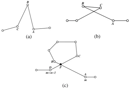
5.2. Alignment Let the point Bbe the point detected

by Eq. (14) which lies between two nodal points Aand

C(see Figure 4a and b). This ill-ordered point is to be

removed, and a new nodal point in alignment is created to replace it. The new nodal point is assigned to be located as:

2

)

(

* C A

B

z

z

z





(16)

A B C A B C A B C D m m+ n+ 1

where

z

may be xor y, and superscript * denotes the new value. Figure 5a and b show the shape of grids after alignment.

(a)

(b)

(c)

Figure 5. Ill-ordered grids (a) out of alignment grid, (b) twisted grid and (c) crossed grid, after alignment

For the case of a crossed grid, as depicted in Figure 4c, the starting point of the first crossed element is connected to the ending point of the second crossed element, and the ill-ordered nodal points are distributed equally over the connecting line. Hence, the locations of ill-ordered points are modified according to the following equation:

n

i

n

z

z

i

z

z

m n m

m i

m

,

1

,

,

1

1

*

























 

 (17)

where n is the number of ill-ordered nodal points. The

modified shape of crossed grid is shown in Figure 5c. In addition to existence of a crossed grid at the adiabatic wall, during the iterative procedure it is possible that the dynamic elements at the adiabatic wall profile cross the static elements at either the design surface or the heater surface. Figure 6a shows such a case where the adiabatic wall profile crossed the design surface. In order to remove the ill-ordered points, the nodal point just before the first cross is connected to the nodal point just after the last cross at the adiabatic wall profile, and the locations of ill-ordered nodal points are

updated based on Eq. (17). Figure 6b shows the

modified grid after alignment.

(a) (b)

Figure 6.Crossing the adiabatic wall with the design surface (a) before alignment, and (b) after alignment

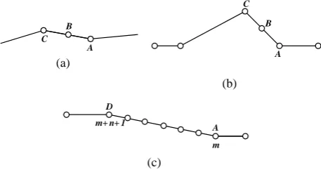
5.3. Redistribution After the alignment step, the nodal points may be distributed in a non-uniform manner, and thus the rate of convergence for iterative procedure may be decreased accordingly. In order to achieve a near uniform grid, we use a redistribution approach. First, the average length of elements is calculated by:

) 1 ( 1

1











M

M

m m

ave 

 (18)

where



_m is the length of the m-th element restricted to

dynamic nodal points m1 and

m

. Then,the number

of segments over the m-th element is determined by:









,

1

,

,

1

NINT







m

M

S

_m



_m



_ave





(19)

here the operator “NINT” rounds its argument to the

nearest integer number, and



is the coefficient of

segmentation. The value of



is selected based on trial

and error process. The value of



is set to be 10 in this

study. Finally, the location of artificial nodal point i at

the m-th element is calculated by:

1

, 1 , 1, , , 1, , 1

m m

m i m m

m

z z

z z i i S m M

S

 

  

  _ _   

    (20)

Therefore, the new number of artificial sub-elements which must be laid between two dynamic nodal points is given by:

  

 _









) 1 ( NINT

1

1 M S

M

m m

 (21)

By defining

1

,

1

, 1, , , 1, , 1 , 1, ,

M

p i j m m

m

w z p S i M j S





  _



 _   _ (22)

The new location of the m-th dynamic nodal point

becomes:

M

m

w

z

m m

,

1

,

,

*







 (23)

with

z

₀*



z

₀ and

z

_M*_1



z

_M1.

Figure 7 shows the locations of the dynamic nodal points at the adiabatic wall before and after redistribution.

Figure 7.The schematic shape of the adiabatic wall profile before and after redistribution

A B C

A B C

A D

m m+ n+ 1

m m+ n+ 1

z3

m m+ n+ 1

(a)

(b)

Figure 8.The geometry of the radiant oven for iteration 13 (a) before regularization and (b) after regularization

Typical regularization procedures for different number of iterations are shown in Figures 8-10. As seen, although the dynamic nodal points are seriously twisted or out of alignment at the start of the regularization procedure, a well-ordered grid distribution can be obtained after few iterations. It is also observed that the uniformity of the element length could be improved through the redistribution.

5.4. The Stopping Criterion The stopping criterion for the iterative procedure of nodal regularization is given by:













M

m

m

m

z

z

1

2

*



(24)

where



is a pre-defined small value.

(a)

(b)

Figure 9.The geometry of the radiant oven for iteration 82 (a) before regularization and (b) after regularization

(a)

(b)

Figure 10.The geometry of the radiant oven for iteration 471 (a) before regularization and (b) after regularization

6. GRID REFINEMENT FOR THE DIRECT PROBLEM

The surface elements of the adiabatic wall may be stretched during the regularization procedure, in such a way that the direct problem of solving the radiative transfer equation is influenced by the discretization error. In order to reduce the discretization error, the surface grid at the adiabatic wall must be refined in each iteration. The refinement approach used in this study is based on the segmentation of surface elements into a number of elements so that the number of sub-elements can be found by:

M m

kmNINTm ave , 1,, (25)

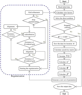
7. OVERALL COMPUTATIONAL ALGORITHM

The overall computational algorithm for shape optimization of a radiant enclosure is shown in Figure 11. The flowchart shows the overall solution procedure containing the direct problem, conjugate gradient method and the nodal regularization approach.

8. RESULTS AND DISCUSSION

The optimization technique based on the CGM and the regularization approach is now demonstrated by applying it for design of a radiant oven as depicted in

Figure 1, for different values of



angle. All the

surfaces are considered to be diffuse-black and the medium is transparent. A uniform heat input,

2

W/m 1 

h

q is posed over the heater surface. The aim of

the design problem is to optimize the geometry of the adiabatic wall to produce a uniform heat flux

x

y

-0.6 -0.3 0 0.3 0.6 0.9 1.2 0

0.3 0.6 0.9 1.2

Design Surface H

ea ter_S

ur_fa ce

x

y

-0.6 -0.3 0 0.3 0.6 0.9 1.2 0

0.3 0.6 0.9 1.2

Design Surface

H ea_te

r_S u rfa ce

x

y

-0.6 -0.3 0 0.3 0.6 0.9 1.2 0

0.3 0.6 0.9 1.2

Design Surface H

ea_te r_S

ur_fa ce

x

y

-0.6 -0.3 0 0.3 0.6 0.9 1.2 0

0.3 0.6 0.9 1.2

Design Surface H

ea_te r S

ur_fa ce

x

y

-0.9 -0.6 -0.3 0 0.3 0.6 0.9 1.2 1.5 1.8 2.1 0

0.3 0.6 0.9 1.2 1.5 1.8 2.1 2.4

H ea_te

r Su

rf_ac e

Design Surface

x

y

-0.9 -0.6 -0.3 0 0.3 0.6 0.9 1.21.5 1.8 2.1 0

0.3 0.6 0.9 1.2 1.5 1.8 2.1 2.4

Design Surface H

distribution of 2

W/m 1  

d

q over the

temperature-specified design surface with an emissive power of

2

W/m 1 

b

E . The design and the heater surfaces are

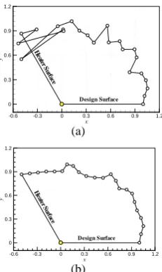
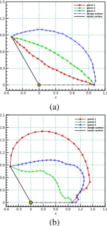
discretized into 10 surface elements, and the adiabatic wall is represented by a suitable number of dynamic nodal points. Figure 12a shows three initial guesses for the adiabatic wall profile of a radiant oven with a

deviation angle of





120

o. The final shapes of the

adiabatic wall for three cases with different initial guesses are shown in Figure 12b. As shown, the obtained profile of adiabatic wall is highly dependent to the initial guess. This conclusion is verified by considering other case with a deviation angle of

o

150





as shown in Fig. 13.

The accuracy of the optimization method is measured by the relative error and the root mean square error which are defined as follows:



_{, ,}



_, 100 ,n dn en dn

rel q q q

Err (26a)





100

1 2 1/2

1

,

,  

  

  









N

n

n e n d

rms q q

N

Err (26b)

The relative error measures the deviation between desired and estimated values on each node, whereas the root mean square error measures the deviation between desired and estimated values over entire extent of the design surface.

The distributions of relative error over the design surface are shown in Figure 14a and b for the cases shown in Figures 12 and 13.

As demonstrated in Figure 14, the accuracy of the optimum shape is highly dependent to the initial guess. However, using a suitable initial guess, the optimum profile may be generated in an acceptable range of error.

Figure 11. The flowchart of the overall computational algorithm

Yes

Start

Read initial data

Solve the direct problem

Yes

End

Existence of ill-ordered grid

Stop regularization

Alignment

Regularization n

Starting the regularization redistribution Existence

of crossed

Grid refinement

Yes Yes

Existence of ill-ordered grid

Yes

Yes

No

No

Alignment

Calculate view factors

No

No

Save the data for iteration



) ( )

(  _ 1

) G Z

Z

Calculate G

Calculate 

Calculate d

Calculate 

No

Save the output data Generate a new set of parameters

No

Calculate sensitivity matrix Stopping

The values of maximum relative error, the root mean square error, the objective function, and the CPU time per iteration for cases with different values of angles of deviation are shown in Table 1. As seen in Table 1, although the maximum relative error for some cases is large, but the values of root mean square error for almost all cases are acceptable.

(a)

(b)

Figure 12.(a) Three initial guesses for adiabatic wall profile, (b) the obtained profiles of the adiabatic wall for three initial guesses, o

120 



(a)

(b)

Figure 13.(a) Three initial guesses for adiabatic wall profile, (b) the obtained profiles of the adiabatic wall for three initial guesses, o

150 



(a)

(b)

Figure 14.The distribution of relative error of estimated heat flux over the design surface for (a) o

120 

 and (b) o

150  

TABLE 1.The maximum relative error, the root mean square error, the objective function and the CPU time per iteration for cases with different angles of deviation and different initial guesses

 Guess Errrel,max

(%)

Errms

(%)

G CPU time (s)

120o

1 3.87 0.018 0.003 1.89

2 65.03 0.413 0.171 1.13

3 4.66 0.029 0.008 1.78

150o

1 3.28 0.017 0.003 2.78

2 14.58 0.0763 0.058 2.54

3 0.96 0.006 0.003 29.33

Moreover, the CPU time is highly dependent to the number of nodal points, and the number of iterations for regularization of the locations of nodal points.

9. CASE STUDY

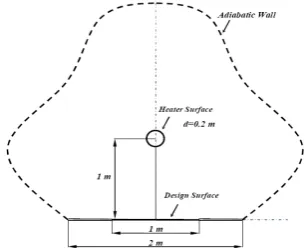
In order to check the performance of shape optimization method for reconstruction of a practical enclosure, we

now consider a design problem of an oven with a 1-m

design surface which is located horizontally at a distance of h1mfrom a cylindrical heater (d=0.2 m), as depicted in Figure 15. The design surface is a

diffuse-gray surface with an emissivity of d0.7 which has a

specified uniform emissive power of 2

/ 1W m

E_d . The

cylindrical heater is diffuse-black and produces a

constant heat flux ofq_h1/(d) W/m2. All other

surfaces are adiabatic. The goal of the design problem is to identify the enclosure configuration to produce the

uniform desired heat flux of 2

/

1W m

qd  over the

design surface.

x

y

-0.6 -0.3 0 0.3 0.6 0.9 1.2 0

0.3 0.6 0.9 1.2 1.5

guess 1 guess 2 guess 3 design surface heater surface

x

y

-0.6 -0.3 0 0.3 0.6 0.9 1.2 1.5 1.8 0

0.3 0.6 0.9 1.2 1.5 1.8 2.1

guess 1 guess 2 guess 3 design surface heater surface

x

y

-1 -0.8 -0.6 -0.4 -0.2 0 0.2 0.4 0.6 0.8 1 1.2 0

0.2 0.4 0.6 0.8 1 1.2 1.4 1.6 1.8

guess 1 guess 2 guess 3 design surface heater surface

x

y

-2.5 -2 -1.5 -1 -0.5 0 0.5 1 1.5 2 2.5 0

0.5 1 1.5 2 2.5 3 3.5 4

4.5 guess 1 guess 2 guess 3 design surface heater surface

x (m)

E

rrre

l

(%

)

0 0.2 0.4 0.6 0.8 1

0 10 20 30 40 50 60 70

guess 1 guess 2 guess 3

  

x (m)

E

rrre

l

(%

)

0 0.2 0.4 0.6 0.8 1

0 2 4 6 8 10 12 14 16

guess 1 guess 2 guess 3

Figure 15.Schematic shape of an enclosure consisting of a cylindrical heater and a design surface located horizontally

Because of symmetry, only half the points constructing the adiabatic wall are considered to be optimized during the iterative regularization approach. The final shape is indicated in Figure 16. The values of objective function, maximum relative error, root mean square error, and the

CPU time per each iteration are reported in Table 2.

Figure 17 shows the distribution of relative error over the design surface. As seen, the desired uniform heat flux distribution over the design surface is well satisfied by optimization of the adiabatic wall.

Figure 16. The obtained geometry for the case shown in Figure 15

Figure 17.The distribution of relative error of estimated heat flux over the design surface for the geometry shown in Figure 16

TABLE 2.The maximum relative error, the root mean square error, the objective function, and the CPU time per iteration for the case described by Figure 15

Errrel,max (%) Errms (%) G CPU time (s)

0.76 0.003 0.0003 14.74

10. CONCLUSION

This article overviewed a gradient-based approach for geometric design of a radiant oven. The primary objective of the work was to find the optimal shape of a radiant enclosure to satisfy the uniform heat flux distribution over the temperature-specified design surface. The radiative transfer equation in the radiant enclosure with diffuse-gray walls, containing a transparent medium was solved by the net radiation method and the view factors were found by the Hottel’s crossed string method. The optimal shape of the enclosure was found by optimizing the locations of dynamic nodal points at the adiabatic wall. The optimization problem was solved by the conjugate gradient method. A regularization approach was posed to the nodal points in order to remove the ill-ordered nodal points and generate a smooth profile. The results show that the optimum shape can be successfully generated by the present method in an acceptable range of error. However, the final solution is highly dependent to the initial guess.

11. REFERENCES

1. Hosseini Sarvari, S.M., Mansouri, S.H. and Howell, J.R., “Inverse boundary design radiation problem in absorbing-emitting media with irregular geometry”, Numerical Heat

Transfer, Part A, Vol. 43, (2003), 565-584.

2. Hosseini Sarvari, S.M., Mansouri, S.H. and Howell, J.R., “Inverse design of three-dimensional enclosures with transparent and absorbing-emitting media using an optimization technique”,

International Communications in Heat and Mass Transfer,

Vol. 30, No. 2, (2003), 149-162.

3. Hosseini Sarvari, Howell, J.R., S.M. and Mansouri, S.H., “Inverse boundary design conduction-radiation problem in irregular two-dimensional domains”, Numerical Heat Transfer,

Part B, Vol. 44, (2003), 209-224.

4. Bayat, N., Mehraban, S. and Hosseini Sarvari, S.M., “Inverse boundary design of a radiant furnace with diffuse-spectral design surface”, International Communications in Heat and Mass

Transfer, Vol. 37, (2010), 103-110.

5. Kirsch, U., “Efficient reanalysis for topological optimization”,

Structural Optimization, Vol. 6, (1993), pp. 143-150.

6. Rodrigues, H. and Fernandes, P., “A material based model for topology optimization of thermoelastic structures”, International

Journal of Numererical Methods in Engineering, Vol. 38,

(1995), 1951-1965.

7. Lampinen, J., “Cam shape optimisation by genetic algorithm”,

Computer-Aided Design, Vol. 35, (2003), 727–737.

8. Yamamoto, K. and Inoue, O., “Applications of genetic algorithm to aerodynamic shape optimization”, Technical Report

AIAA-95-1650-CP, AIAA, (1995).

9. Peigin, S. and Epstein, B., “Robust optimization of 2-d airfoils driven by full navier-stokes computations”, Computational

Fluids, Vol. 33, (2004), 1175–1200.

10. Malekzadeh, P., Rahideh, H. and Karami, G., “optimization of convective–radiative fins by using differential quadrature element method”, Energy Conversion and Management, Vol. 47, (2006), 1505-1514.

11. Malekzadeh, P., Rahideh, H. and Setoodeh, A.R., “Optimization of non-symmetric convective–radiative annular fins by differential quadrature method”, Energy Conversion and

Management, Vol. 48, (2007), 1671-1677.

x

y

-2 -1.5 -1 -0.5 0 0.5 1 1.5 2

-0.5 0 0.5 1 1.5

Design Surface Heater Surface

x (m)

E

rrre

l

(%

)

-0.5 -0.4 -0.3 -0.2 -0.1 0 0.1 0.2 0.3 0.4 0.5

12. Kundu, B. and Das, P.K., “Optimum profile of thin fins with volumetric heat generation: a unified approach”, ASME Journal

of Heat Transfer, Vol. 127, (2005), 945-948.

13. Fabbri, G., “A genetic algorithm for fin profile optimization”,

International Journal of Heat and Mass Transfer, Vol. 72,

(1997), 2165-2172.

14. Fabbri, G., “Heat transfer optimization in internally finned tubes under laminar flow conditions”, International Journal of Heat

and Mass Transfer, Vol. 41, (1998), 1243-1253.

15. Azarkish, H., Hosseini Sarvari, S.M. and Behzadmehr, A., “Optimum geometry design of a longitudinal fin with volumetric heat generation”, Energy Conversion and Management, Vol. 51, (2010), 1938-1946.

16. Hosseini Sarvari, S.M., “Optimal geometry design of radiative enclosures using the genetic algorithm”, Numerical Heat

Transfer, Part A, Vol. 52, (2007), 127-143.

17. Fletcher, R., “Practical methods of optimization” 2nd_{Ed., John}

Wiley & Sons, New York, (2001).

18. Daun, K. J., Howell, J. R., and Morton, D. P., “Geometric optimization of radiative enclosures through nonlinear programming”, Numerical Heat Transfer, Part B, Vol. 43, (2003), 203–219.

19. Daun, K. J., Morton, D. P., and Howell, J. R., “Geometric optimization of radiant enclosures containing specular surfaces”,

ASME Journal of Heat Transfer, Vol. 125, (2003), 845–85.

20. Lan, C.H., Cheng, C.H., and Wu, C.Y., “Shape design for heat conduction problems using curvilinear grid generation conjugate gradient, and redistribution methods”, Numerical Heat Transfer,

Part A, Vol. 39, (2001), 487-510.

21. Siegel, R. and Howell, J.R., “Thermal radiation heat transfer”, 4th Ed., Taylor and Francis, (2002).

Optimum Shape Design of a Radiant Oven by the Conjugate Gradient Method and a

Grid Regularization Approach

M. Jahanbakhsh Rostamia_{, S.M. Hosseini Sarvari}b *_{, A. Behzadmehr}a

a

Mechanical Engineering Department, The University of Sistan & Baluchestan, 98135-161, Zahedan, Iran Mechanical Engineering

b_{Department, Shahid Bahonar University of Kerman,76175-133, Kerman, Iran}

A R T I C L E I N F O

Article history:

Received 9 June 2011

Accepted in revised form 17May2012

Keywords:

Inverse Geometry Design Radiation

Optimization

هﺪﯿﮑﭼ

ﯽﺸﺨﭘ حﻮﻄﺳ و فﺎﻔﺷ ﻂﯿﺤﻣ ﺎﺑ ﯽﺸﺑﺎﺗ ﻪﻈﻔﺤﻣ ﮏﯾ ﯽﺣاﺮﻃ ﺖﻬﺟ يزﺎﺳ ﻪﻨﯿﻬﺑ ﻪﻠﺌﺴﻣ ﮏﯾ ﻪﻌﻟﺎﻄﻣ ﻦﯾا رد

-ﺖﺳا هﺪﺷ ﻪﺋارا يﺮﺘﺴﮐﺎﺧ .

تﺎﻋﻼﻃا زا هدﺎﻔﺘﺳا ﺎﺑ ﯽﺸﺑﺎﺗ ﻪﻈﻔﺤﻣ ﮏﯾ ﻪﻨﯿﻬﺑ ﻪﺳﺪﻨﻫ ﻦﺘﻓﺎﯾ ﯽﺣاﺮﻃ ﻪﻠﺌﺴﻣ فﺪﻫ

ﺢﻄﺳ زا ﯽﯾﺎﻫ ﺖﻤﺴﻗ يور ﯽﺗراﺮﺣ رﺎﺷ و ﺎﻣد ﺪﺷﺎﺑ ﯽﻣ دراد مﺎﻧ ﯽﺣاﺮﻃ ﺢﻄﺳ ﻪﮐ يزﺮﻣ

. تراﺮﺣ لﺎﻘﺘﻧا ﻞﺣ

ﺎﺑ ﻞﺗﺎﻫ ﻊﻃﺎﻘﺘﻣ يﺎﻫرﺎﺗ شور زا هدﺎﻔﺘﺳا ﺎﺑ ﻞﮑﺷ ﺐﯾاﺮﺿ نآ رد ﻪﮐ ﺖﺳا ﺺﻟﺎﺧ ﺶﺑﺎﺗ شور سﺎﺳاﺮﺑ ﯽﺸﺑﺎﺗ ﺪﻨﯾآ ﯽﻣ ﺖﺳﺪﺑ بﺪﺤﻣ حﻮﻄﺳ و ﻊﻧاﻮﻣ ﻦﺘﻓﺮﮔ ﺮﻈﻧرد .

،فﺪﻫ ﻊﺑﺎﺗ ﮏﯾ ندﺮﮐ ﻪﻨﯿﻤﮐ رﻮﻈﻨﻤﺑ جودﺰﻣ ﺐﯿﺷ شور

ﺘﺧا تﺎﻌﺑﺮﻣ عﻮﻤﺠﻣ ترﻮﺼﺑ ﻪﮐ ﻒﯾﺮﻌﺗ ﯽﺣاﺮﻃ ﺢﻄﺳ يور هﺪﺷ ﯽﺑﺎﯾزرا و بﻮﻠﻄﻣ ﯽﺗراﺮﺣ يﺎﻫرﺎﺷ ﻦﯿﺑ فﻼ

دﺮﯿﮔ ﯽﻣ راﺮﻗ هدﺎﻔﺘﺳا درﻮﻣ ،دﻮﺷ ﯽﻣ .

ﺪﻧﻮﺷ ﯽﻣ ﻪﺒﺳﺎﺤﻣ دوﺪﺤﻣ فﻼﺘﺧا شور زا هدﺎﻔﺘﺳا ﺎﺑ ﺖﯿﺳﺎﺴﺣ ﺐﯾاﺮﺿ .

ﯽﻣ ﻞﻤﻋ يراﺮﮑﺗ ﺪﻨﯾآﺮﻓ ﮏﯾ رد ﻪﮐ ﺖﺳا هﺪﺷ ﻪﺋارا ﻪﺘﺨﯾر ﻢﻫرد يﺎﻫ هﺮﮔ ﻢﯿﻈﻨﺗ ﺖﻬﺟ ﯽﻤﯿﻈﻨﺗ رﺎﮑﻫار ﮏﯾ ﺪﻨﮐ . ﻈﻨﻤﺑ ﺖﺳا هﺪﯾدﺮﮔ ﻪﺋارا ﯽﯾﺎﻫ لﺎﺜﻣ شور ﺖﻗد و دﺮﮑﻠﻤﻋ ﺶﯾﺎﻤﻧ رﻮ .

ﻪﻨﯿﻬﺑ ﻪﺳﺪﻨﻫ ﻪﮐ ﺪﻫد ﯽﻣ نﺎﺸﻧ ﺞﯾﺎﺘﻧ

دﻮﺷ ﺪﯿﻟﻮﺗ ﺪﻧاﻮﺗ ﯽﻣ ﺰﯿﻣآ ﺖﯿﻘﻓﻮﻣ يا ﻪﻧﻮﮕﺑ ﯽﺸﺑﺎﺗ ﻪﻈﻔﺤﻣ .