TECHNICAL NOTE
RELIABILITY ANALYSIS OF K-OUT-OF N: G MACHINING
SYSTEMS WITH MIXED SPARES AND MULTIPLE
MODES OF FAILURE
Madhu Jain*, G. C. Sharma and Ranjeet Singh Pundhir Department of Mathematics, Institute of Basic Science Dr. B. R. Ambedkar University, Khandari, St. John’s College
Agra-282002, India
[email protected] - [email protected]
*Corresponding Author
(Received: November 30, 2006 - Accepted in Revised Form: September 13, 2007)
Abstract This paper deals with the transient analysis of K-out-of-N: G system consisting of N-operating machines. To improve system reliability, Y cold standby and S warm standbys spares are provided to replace the failed machines. The machines are assumed to fail in multiple modes. At least K-out-of-N machines for smooth functioning of the system. Reliability and mean time to failure are established in terms of transient probabilities.
Keywords K-Out-of-N: G System, Mixed Spares, Reliability, MTTF, Multiple Failure Modes
ﻩﺪﻴﮑﭼ
ﺩﺭﻮﻣﺭﺩﻪﻟﺎﻘﻣﻦﻳﺍ
ﻱﺍﺭﺬﮔﻞﻴﻠﺤﺗﻭﻪﻳﺰﺠﺗ
ﻢﺘﺴﻴﺳﻚﻳ
K
ﺯﺍ
N:G
ﻞﻣﺎﺷ
N
ﯽﺗﺎﻴﻠﻤﻋﻦﻴﺷﺎﻣ ﻲﻣ
ﺪﺷﺎﺑ
.
ﺭﻮﻈﻨﻣﻪﺑ
ﺩﻮﺒﻬﺑ ﻲﻳﺎﻳﺎﭘ
،ﻢﺘﺴﻴﺳ
Y
ﻭﻝﺎﻌﻓﻭﺭﺯﺭﻦﻴﺷﺎﻣ
S
ﻲﻨﻳﺰﮕﻳﺎـﺟﻱﺍﺮﺑﻝﺎﻌﻓﺮﻴﻏﻭﺭﺯﺭﻦﻴﺷﺎﻣ ﺎﻣ
ﻦﻴـﺷ
ﻱﺎـﻫ
ﻩﺪﺷﺏﺍﺮﺧ
ﺖﺳﺍﻩﺪﺷﻢﻫﺍﺮﻓ
.
ﻦﻴﺷﺎﻣﻲﺑﺍﺮﺧ
ﺪﻨﭼﺭﺩﺎﻫ ﺖﻟﺎﺣ
ﻩﺪﺷﺽﺮﻓ
ﺍ ﺖﺳ
ﻞﻗﺍﺪﺣﻭ
K
ﺯﺍ
N
ﻦﻴﺷﺎﻣ ﯼﺍﺮـﺑ
ﻲﻣﺯﺎﻴﻧﺩﺭﻮﻣﻢﺘﺴﻴﺳﻱﺯﺎﺳﺭﺍﻮﻤﻫ
ﺪﺷﺎﺑ
. ﺍﺭﺬـﮔﺕﻻﺎـﻤﺘﺣﺍﺯﺍﻩﺩﺎﻔﺘﺳﺍﺎﺑﻢﺘﺴﻴﺳﻲﺑﺍﺮﺧﺎﺗﻥﺎﻣﺯﻂﺳﻮﺘﻣﻭﻲﻳﺎﻳﺎﭘ
ﻩﺪﺷﻒﻳﺮﻌﺗ ﺪﻧﺍ
.
1. INTRODUCTION
The performance of any machining system is highly influenced by machine failure. The machine failure may be balanced either by providing spare part support or by facilitating better repair or both so that the production may not suffer. Reliability indices of K-out of-N: G machining system with spares has been studied by many researchers. Teixeirade [1] presented multi-criteria decision models for two maintenance problems in which one is a repair contract selection and other one is a spares provisioning. Arulmozhi [2] developed a closed form solution for the system reliability of an M-out of-N warm standby system with R repairmen. Amri et al. [3]
considered optimal design of k-out-of-n: G subsystems subjected to imperfect fault-coverage. Zhang et al. [4] obtained availability and reliability of k-out-of-(M+N): G warm standby systems.
Sharma [7] considered M/M/R machine repair problem with spares and three modes of failure. Wang and Lee [8] developed the Cold-standby M/M/R machine repair problem where a group of identical and independent operating machines have K(K ≥1) failure modes. The cost analysis of the M/M/R machine repair problem with two modes of failure was provided by Wang and Wu [9] and Jain et al. [10]. Levitin [11] developed a model, which generalizes the linear consecutive k-out-of-r-from-n system to the case of multiple failure criteria. Assessment of reversible multi-state k-out-of-n: a G/F load-sharing system was discussed by Jenab and Dhillon [12] by using flow-graph models.
2. MODEL DESCRIPTION
A K-out-of N: G machining systems was considered with mixed spares and multiple modes of failure. The following assumptions and notations have been used for mathematical formulation of the problem:
• The system consists of N operating machines and Y cold standbys and S warm standbys.
• The life time and repair time of the machines are exponentially distributed. • There is a provision of cold standbys and
warm standbys to replace the failed machines.
• The total number of machines in the system is given by L = N + Y + S.
• Whenever a machine is repaired, it becomes as good as a new one.
• The system works if at least K machines are working.
• The machine may fail in any one of M modes of failure. Repair times of the machine failed in mth (m = 1, 2, …, M)
mode are exponentially distributed with rates μm.
• mth (m = 1, 2, …, M) failure mode of
operating machines are independent Poisson processes. The state dependent rates are given by
⎪ ⎪ ⎩ ⎪⎪ ⎨ ⎧
− < ≤ + −
+ +
+ < < −
+ +
≤ ≤ +
=
K L j Y S , m λ' j) Y S N (
Y S j Y , m α j) S (Y m λ N
Y j 0 ,
m Sα m λ N
λ(j) (1)
where λm and αm are mean failure rates of
operating and warm standby machines in mth
mode (m = 1, 2, …, M), respectively; λ'm (m = 1, 2,…, M) is the degraded mean failure rate of operating machines in mth mode when there are less than N operating machine in the system.
3. SYSTEM WITH REPAIR
The mathematical model for the relevant system can be formulated as a continuous time parameter. The Morkov chain with states (jem) (j = 0, 1, …,
N-K+1) representing the number of failed components due to mth failure mode; here em is a
unit row of dimension M having unity at the mth
position and zero elsewhere. Let Pt (jem) denote the
probability of this state at time t. Also denote
∑ =
= M
1
m m
λ
λ , ∑
=
= M
1
m m
α
α .
When the system starts at time t = 0 in the state (0), the set of differential equations are as given below:
[
]
∑= + +
−
= M
1 m
) m (e t P m μ (0)
t P Sα Nλ dt
(0) t dP
(2)
[
]
[
]
(
1 j Y)
, ) m e ) 1 j (( t P m μ 1) (j
) m e 1) ((j t P m α S m λ N
) m (je t P m jμ m Sα m Nλ dt
) m (je t dP
≤ ≤ +
+
+ −
+
+ +
+ −
=
(3)
[
]
[
]
(
Y j Y S)
, ) m 1)e ((j t P
m α ) 1) j ( S Y ( m Nλ
) m 1)e ((j t P m μ 1) (j
) m (je t P m jμ m α ) j S Y ( m λ N dt
) m (je t dP
+ < < −
− − + +
+ +
+
+ +
− + + −
=
[
Nλm (Y S (j 1))αm]
Pt((j 1)em),(j Y S). ) m 1)e j (( t P m μ 1) (j ) m je ( t P m jμ m ' j)λ Y S N ( dt ) m (je t dP + = − − − + + + + + + ⎥⎦ ⎤ ⎢⎣ ⎡ + + − + − = (5)(
Y S j L K)
), m 1)e ((j t P m μ 1) (j ) m 1)e ((j t P m ' 1))λ (j (L ) m (je t P m jμ m ' j)λ (L dt ) m (je t dP − < < + + + + − ⎥⎦ ⎤ ⎢⎣ ⎡ − − + ⎥⎦ ⎤ ⎢⎣ ⎡ − + − = (6)
(
j L K)
), m e 1) j (( t P m ' λ ) 1) (j L ( ) m je ( t P m jμ m ' λ j) L ( dt ) m (je t dP − = − ⎥⎦ ⎤ ⎢⎣ ⎡ − − + ⎥⎦ ⎤ ⎢⎣ ⎡ − + − = (7) 1) K -(L j ), m K)e ((N t P m ' Kλ dt ) m 1)e K ((N t dP + = − = + − (8)
where the initial conditions are: 0 j for 0 ) m (je 0 P and 1 (0) 0
P = = > (9)
The reliability R(t) with repair and mean time to failure (MTTF) of the system can be calculated using ∑− + + = ∑= ∑ − + = ∑= + + ∑ = ∑= + = 1 S Y 1 Y j M 1 m K L S Y j M 1
m Pt (jem) ) m je ( t P Y 1 j M 1 m ) m je ( t P (0) t P repair) (with t R (10) and ∫ ∞ = 0 dt repair) (with t R MTTF (11)
4. SYSTEM RELIABILITY WITHOUT REPAIR
If μm = 0, then it is a case without repair and the
following recursive formulae can be derived. It can be denoted that the Laplace transforms of Pt (jem)
by Pˆs( jem); 0≤ j≤L-K+1. Taking Laplace transform of Equations 2-8,
[
s Nλ Sα]
1 (0) s Pˆ + +
= , j = 0 (12)
(
)
(
1 j Y)
, j m Sα m λ N s m Sα m Nλ Sα Nλ s 1 ) m (je s Pˆ ≤ ≤ ⎪ ⎭ ⎪ ⎬ ⎫ ⎪ ⎩ ⎪ ⎨ ⎧ ⎥⎦ ⎤ ⎢⎣ ⎡ + + ⎥⎦ ⎤ ⎢⎣ ⎡ + + + = (13)
(
)
(
)
[
]
(
)
[
]
(
Y j Y S)
, j 1 Y n m α n S Y m λ N s j 1 Y n m α 1) (n S Y m λ N Y m α S m λ N s m α S m λ N Sα Nλ s 1 ) m (je s Pˆ + < < ∏ + = + + + − ∏ + = + + − − ⎪ ⎭ ⎪ ⎬ ⎫ ⎪ ⎩ ⎪ ⎨ ⎧ ⎥⎦ ⎤ ⎢⎣ ⎡ + + ⎥⎦ ⎤ ⎢⎣ ⎡ + + + = (14)
(
)
(
)
(
)
{
}
(
Y S j L K)
Now inverting the Laplace transforms from Equations 9-12, 0 j , t ) α S λ N ( e (0) t
P = − + = (16)
Using 1)! (n at e 1 n t n a) (s 1 1 L − − − = ⎟ ⎟ ⎠ ⎞ ⎜ ⎜ ⎝ ⎛ +
− and convolution
theorem, we have
(
)
(
)
(
1 j Y)
, 2 ) m α α S( ) m λ λ ( N 1 t ) m α (α S ) m λ λ ( N e 1)! (Y ) m α α S( ) m λ λ ( N t ) m α S(α ) m λ λ ( N e 1 Y t ! 1 Y t Sα λ N e Y m α S m λ N ) m je ( t P ≤ ≤ ⎥ ⎥ ⎥ ⎥ ⎥ ⎥ ⎥ ⎥ ⎥ ⎥ ⎥ ⎦ ⎤ ⎢ ⎢ ⎢ ⎢ ⎢ ⎢ ⎢ ⎢ ⎢ ⎢ ⎢ ⎣ ⎡ ⎥⎦ ⎤ ⎢⎣ ⎡ − + − ⎪⎭ ⎪ ⎬ ⎫ ⎪⎩ ⎪ ⎨ ⎧ − − + − − − ⎥⎦ ⎤ ⎢⎣ ⎡ − + − − + − − − + − ⎟ ⎠ ⎞ ⎜ ⎝ ⎛ + = ⎥⎦ ⎤ ⎢⎣ ⎡ ⎥ ⎥ ⎦ ⎤ ⎢ ⎢ ⎣ ⎡ (17)
(
)
[
(
)
]
(
)
(
)
(
)
{
}
(
)
[
]
[
]
[
]
(
)
(
)
(
)
⎪ ⎪ ⎪ ⎪ ⎨ ⎧ × ⎥⎦ ⎤ ⎢⎣⎡ λ+ α − λ + + − α
α − + + λ − ∑ + = + ⎢ ⎢ ⎢ ⎢ ⎢ ⎢ ⎢ ⎢ ⎢ ⎢ ⎢ ⎢ ⎢ ⎢ ⎢ ⎣ ⎡ ⎪ ⎪ ⎪ ⎪ ⎪ ⎪ ⎪ ⎭ ⎪ ⎪ ⎪ ⎪ ⎪ ⎪ ⎪ ⎬ ⎫ ⎪ ⎪ ⎪ ⎪ ⎪ ⎪ ⎪ ⎩ ⎪ ⎪ ⎪ ⎪ ⎪ ⎪ ⎪ ⎨ ⎧ ⎥ ⎥ ⎥ ⎥ ⎥ ⎥ ⎥ ⎥ ⎥ ⎦ ⎤ ⎢ ⎢ ⎢ ⎢ ⎢ ⎢ ⎢ ⎢ ⎢ ⎣ ⎡ α − α + λ − λ ⎪⎭ ⎪ ⎬ ⎫ ⎪⎩ ⎪ ⎨ ⎧ − α − α + λ − λ − − α − α + λ − λ α − α + λ − λ − × ∏ +
= λ + + − α − λ+ α
α + λ − × − ∏ +
= λ + + − − α
α + λ = ⎥ ⎥ ⎦ ⎤ ⎢ ⎢ ⎣ ⎡ ⎥⎦ ⎤ ⎢⎣ ⎡ ⎥⎦ ⎤ ⎢⎣ ⎡ } m n S Y m N { S N t m n S N m N e j 1 Y n 2 ) m ( S ) m ( N 1 t ) m ( S ) m ( N e )! 1 Y ( ) m ( S ) m ( N t ) m ( S ) m ( N e 1 Y t j 1 Y n S N m n S Y m N t S N e ! 1 Y j 1 Y n m ) 1 n ( S Y m N Y m S m N ) m je ( t P
(
)
(
)
[
]
S Y j Y , 2 m ) n N ( 1 t m ) n N ( e ! ) 1 Y ( m ) n N ( t m ) n N ( e 1 Y t j n p 1 Y n m p S Y m n S Y 1 + < ≤ ⎥ ⎥ ⎥ ⎥ ⎥ ⎥ ⎥ ⎥ ⎥ ⎦ ⎤ ⎪ ⎪ ⎪ ⎪ ⎭ ⎪ ⎪ ⎪ ⎪ ⎬ ⎫ ⎥ ⎥ ⎥ ⎥ ⎥ ⎥ ⎥ ⎥ ⎦ ⎤ α − ⎪ ⎭ ⎪ ⎬ ⎫ ⎪ ⎩ ⎪ ⎨ ⎧ − α − − ⎢ ⎢ ⎢ ⎢ ⎢ ⎣ ⎡ − α − α − − × ∏ ≠ += + − α − + − α
⎥⎦ ⎤ ⎢⎣ ⎡ ⎥ ⎥ ⎦ ⎤ ⎢ ⎢ ⎣ ⎡ ⎥⎦ ⎤ ⎢⎣ ⎡ ⎥ ⎥ ⎦ ⎤ ⎢ ⎢ ⎣ ⎡ (18)
(
)
[
(
)
]
[
]
(
Y 1)
! j S Y n m ' ) 1 n ( L S Y 1 Y n m ) 1 n ( S Y m N Y m S m N ) m je ( t P − ∏ += − − λ
∏+ +
= λ + + − − α
α + λ =
(
)
(
)
{
}
(
)
[
]
[
]
⎪ ⎪ ⎪ ⎭ ⎪ ⎪ ⎪ ⎬ ⎫ ⎥ ⎥ ⎥ ⎥ ⎥ ⎥ ⎥ ⎦ ⎤ α − α + λ − λ ⎪⎭ ⎪ ⎬ ⎫ ⎪⎩ ⎪ ⎨ ⎧ − α − α + λ − λ − ⎢ ⎢ ⎢ ⎢ ⎢ ⎣ ⎡ − ⎥⎦ ⎤ ⎢⎣⎡ λ−λ + α−α
α − α + λ − λ − × ∏ + = ⎥⎦ ⎤ ⎢⎣
⎡ − λ
∏− +
+
= λ + + − α − λ+ α
⎢ ⎢ ⎣ ⎡ ⎩ ⎨
⎧ − λ+ α
(
)
(
)
{
(
)
}
(
)
(
)
(
)
(
)
[
]
⎪⎭ ⎪ ⎬ ⎫ ∏ += − λ − λ − + − α
⎥ ⎥ ⎥ ⎥ ⎥ ⎥ ⎥ ⎦ ⎤ ⎢ ⎢ ⎢ ⎢ ⎢ ⎢ ⎢ ⎣ ⎡ α − ⎪⎭ ⎪ ⎬ ⎫ ⎪⎩ ⎪ ⎨ ⎧ − α − − − α − α − − × ∏− + ≠ + = ⎥⎦ ⎤ ⎢⎣
⎡ + − α − + − α
⎥⎦ ⎤ ⎢⎣
⎡ λ+ α − λ + + − α
⎪ ⎩ ⎪ ⎨
⎧ − λ + + − α
∑− + + = + ⎥⎦ ⎤ ⎢⎣ ⎡ ⎥⎦ ⎤ ⎢⎣ ⎡ ⎥⎦ ⎤ ⎢⎣ ⎡ ⎥⎦ ⎤ ⎢⎣ ⎡ ⎥⎦ ⎤ ⎢⎣ ⎡ j S Y n m n S Y m N m ' n L 2 m ) n N ( 1 t m ) n N ( e )! 1 Y ( m ) n N ( t m ) n N ( e 1 Y t 1 S Y n r 1 Y n m r S Y m n S Y m n S Y m N S N t m n S N m N e 1 S Y 1 Y n
(
) (
)
[
]
(
)
{
}
(
)
(
)
(
)
[
]
K L j S Y , j q n S Y n m ' q L m ' n L 2 m S m N m ' ) n L ( 1 t m S m N m ' ) n L ( e ! ) 1 Y ( m S m N m ' ) n L ( t m S m N m ' ) n L ( e 1 Y t m ' n L m n S Y m N 1 S Y 1 Y n } m ' n L { S N t m ' ) n L ( e j S Y n − ≤ ≤ + ⎥ ⎥ ⎥ ⎥ ⎥ ⎥ ⎥ ⎥ ⎥ ⎦ ⎤ ⎪ ⎪ ⎪ ⎪ ⎭ ⎪ ⎪ ⎪ ⎪ ⎬ ⎫ ∏ ≠ += − λ − − λ
⎥ ⎥ ⎥ ⎥ ⎥ ⎥ ⎥ ⎦ ⎤ α + λ − λ − ⎪⎭ ⎪ ⎬ ⎫ ⎪⎩ ⎪ ⎨ ⎧ − α + λ − λ − − ⎢ ⎢ ⎢ ⎢ ⎣ ⎡ − α + λ − λ − α + λ − λ − − × ⎥⎦ ⎤ ⎢⎣
⎡ λ + + − α − − λ
∏− + + = λ − − α + λ λ − − ⎪⎩ ⎪ ⎨ ⎧ ∑ + = + ⎥ ⎦ ⎤ ⎢ ⎣ ⎡ ⎟ ⎠ ⎞ ⎜ ⎝ ⎛ ⎥ ⎦ ⎤ ⎢ ⎣ ⎡ ⎟ ⎠ ⎞ ⎜ ⎝ ⎛ ⎥ ⎦ ⎤ ⎢ ⎣ ⎡ ⎟ ⎠ ⎞ ⎜ ⎝ ⎛ ⎥ ⎦ ⎤ ⎢ ⎣ ⎡ ⎟ ⎠ ⎞ ⎜ ⎝ ⎛ ⎥⎦ ⎤ ⎢⎣ ⎡ (19)
The transient reliability R(t) and mean time to failure (MTTF) of the system without repair can be calculated by using the similar formulae as given in Equations 10-11.
5. SYSTEM RELIABILITY FOR MODIFIED MODEL WITH REPAIR
In this case, the reliability system is considered with repair as in Section 3 including the assumption that the relations between two failure modes are permissible. Let ∑
= = M 1 m J m e m
j be the state of the system representing the number of failed components due to failure mode-m and Pt(J) be the probability of the system state at time t. For state 0, Equation 2 holds. Now other equations are constructed as follows:
K L j S Y , ) m e J ( t P m μ ) 1 m j ( M
1 m π
) m e J ( t P m 1)) (J L (
) J ( t P m μ m j M
1 m m ' λ ) J L ( dt
(J) t dP
− < < + +
+ ∑
=
+ − ⎥⎦ ⎤ ⎢⎣
⎡ − − λ′
+ ⎥
⎥ ⎦ ⎤ ⎢
⎢ ⎣ ⎡
∑ = + −
− =
(23)
K L j ), m e J ( t P m λ' 1)) (J (L
) J ( t P M
1
m m
μ m j m
λ' ) J L ( dt
) m je ( t P d
− = −
⎥⎦ ⎤ ⎢⎣
⎡ − −
+
⎥ ⎥ ⎦ ⎤ ⎢
⎢ ⎣ ⎡
∑ = + −
− =
(24)
[
]
) 1 K -L ( j )), m e (J L ( t P
m λ' ) m je ( ψ M
1 m 1) (J L dt
(J) t P d
+ =
− −
∑ = − − =
(25)
Where
⎪⎩ ⎪ ⎨ ⎧
> = =
0 m j 1,
0 m j , 0 ) m je
ψ( (26)
⎩ ⎨ ⎧
− <
− = =
π
K N J , 1
K N J , 0
(27)
The initial conditions are same as given by Equation 9.
The reliability R(t) and mean time to failure (MTTF) of the system can be calculated using Equation 10 and 11.
6. SPECIAL CASES
Now consider the special cases by setting appropriate parameters as follows:
Case I
Model With Two Modes Of Failure
Here the
machines are failed in two modes (i.e. M = 2). In this case, the formulae for reliability with and without repair, which coincide with the result
obtained by Moustafa is obtained (1996).
Case II
Model With Multiple Modes of Failure Without Spare
When S = 0, Y = 0, in this case the system
reliability without spares is found. In this case the present model reduces to the model studied by Moustafa.
7. NUMERICAL ILLUSTRION
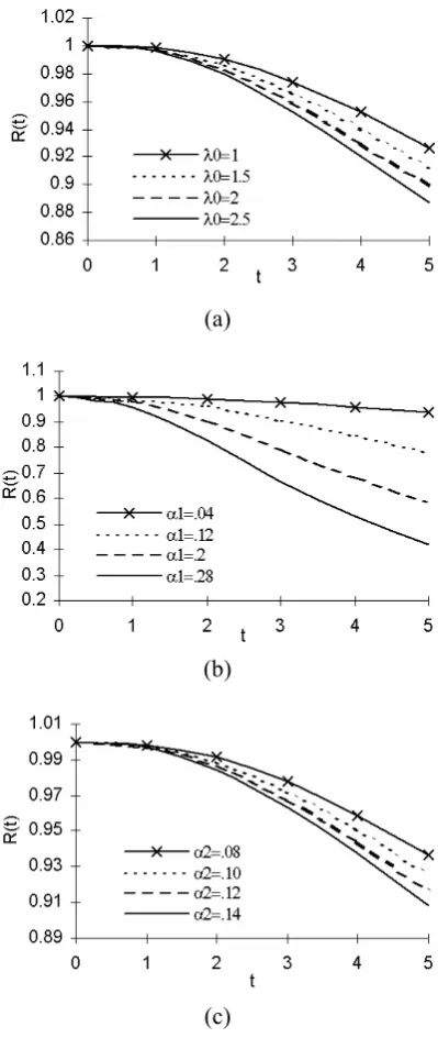
Numerical illustrations have been made to calculate system reliability. The system reliability profiles for the model with repair for different values of λ0, α1 and α2 are displayed in Figures
1(a)-1(c) for heterogeneous Figures 2(a)-2(c) exhibit the system reliability for the model without repair with a heterogeneous rate. In all these figures, the default parameters are fixed as follows: From Figures 1(a)-1(c) and 2(a)-2(c) a lower value of t,R(t) is observed that decreases slowly but as t takes higher values, there is a sharp decrease in R(t). Also as λ0, α1 and α2 increase, the reliability
decreases, the effect is more prominent as time increases.
8. CONCLUSIONS
(a)
(b)
(c)
Figure 1. System reliability for model with repair and
heterogeneous rate by varying (a) λ0 (b) α1 (c) α2.
(a)
(b)
(c)
Figure 2. System reliability for model without repair and
heterogeneous rate by varying (a) λ0 (b) α1 (c) α2.
failures; the average message load may be such that at least two transmitters must be operational at all times otherwise critical messages will be lost. The present study can be extended for linear and consecutive k-r-out-of-n: G system; the other generalization can be done by incorporating
common cause of failure.
9. REFERENCES
maintenance spares and contracts planning”, European Journal of Operational Research, Vol. 129, No. 2,
(2001), 235-241.
2. Arullnozhi, G., “Reliability of an M-out of-N warm standby system with R repair facilities”, OPSEARCH,
Vol. 39, (2002), 77-87.
3. Amari, S. V., Pham, H. and Dill, G., “Optimal design of k-out-of-n: G subsystems subject to imperfect fault-coverage”, IEEE Transaction on Reliability, Vol. 53
No. 4, (2004), 567-575.
4. Zhang, T., Xie, M. and Horigome, M., “Availability and reliability of k-out-of-(M+N): G warm standbys systems”, Reliability Engineering and System Safety,
Vol. 91, No. 4, (2006), 381-387.
5. Goel, L. R. and Sharma, G. C., “Stochastic analysis of a two unit standby system with two failures and slow switch”, Microelectronics and Reliability, Vol. 29, No.
4, (1980), 493-498.
6. Reddy, D. R. and Rao, D. V. B., “Optimization of parallel systems subjects to two modes of failure and repair provision”, OPSEARCH, Vol. 29, (1993),
25-35.
7. Sharma, D. C. and Sharma, G. C., “M/M/R machine repair problem with spare and three modes of failures”,
Ganita Sandesh, Vol. 11, No. 1, (1997), 51-56.
8. Wang, K. H. and Lee, H. C., “Cost analysis of the
cold-standby M/M/R machine repair problem with multiple modes of failure”, Microelectronics and Reliability,
Vol. 38, No. 3, (1998), 435-441.
9. Wang, K. H. and Wu, J. D., “Cost analysis of the M/M/R machine repair problem with spares and two modes of failure”, Journal of Operations Research Society, Vol. 46, (1995), 783-790.
10. Jain, M., Singh, M. and Baghel, K. P. S., “Machine repair problem with spares, reneging, additional repairman and two modes of failure”, Journal of MACT, Vol. 33, (2000), 69-79.
11. Levitin, Gregory, “Consecutive k-out-of-r-from-n system with multiple failure criteria”, IEEE Transaction on Reliability, Vol. 53, No. 3, (2004), 394-400.
12. Jenab, K. and Dhillon, B. S., “Assessment of reversible
multi-state k-out-of-n: G/F/Load-Sharing systems with flow-graph models”, Reliability Engineering and System Safety, Vol. 91, No. 7, (2006), 765-771.
13. Moustafa, M. S., “Transient analysis of reliability with and without repair for k-out-of n: G system with M failure modes”, Reliability Engineering and System Safety, Vol. 59, (1998), 317-320.