RESEARCH NOTE
NONLINEAR SENSITIVITY ANALYSIS OF RCMRF
CONSIDERING BOTH AXIAL AND
FLEXURE EFFECTS
A.R. Habibi
Department of Civil Engineering, University of Kurdistan P.O. Box 416, Sanandaj, Iran
(Received: February 07, 2010 – Accepted in Revised Form: September 15, 2011) doi:10.5829/idosi.ije.2011.24.03a.02
Abstract Sensitivity analysis of structures considering their nonlinear behavior has recently been an important process in optimal design of them based on new design concepts such as Performance-Based Design (PBD). The main objective of this research is to develop an efficient and applicable method for nonlinear sensitivity analysis of Reinforcement Concrete Moment Resisting Frames (RCMRF) considering both axial and flexure effects under seismic loading. For this purpose, sensitivity equations are firstly derived based on pushover method, which is a powerful tool for nonlinear analysis of structures in the PBD context, and then a procedure for nonlinear sensitivity analysis is proposed. The results of the method are compared with nonlinear sensitivity results considering only flexural effect and those of Finite Difference Method (FDM). It is shown that existence of axial forces can affect sensitivity coefficients with respect to the design variables. Keywords Nonlinear, Sensitivity, Analysis, Pushover, RCMRF, PBD, Axial and Flexure Effects, Seismi
1. INTRODUCTION
Considerable part of computational effort in an optimization problem is usually allocated to the sensitivity analysis. Each sensitivity coefficient defines the amount of change in a structural response due to a unit change in a design variable, such as sensitivity of displacement to change in cross-sectional dimensions or reinforcement ratio. In recent years, new design concepts such as performance-based design have become a necessity for design of new structures. Since
nonlinear methods such as pushover analysis are used in these new design concepts, it is necessary that efficient nonlinear sensitivity methods be employed in optimum design.
While considerable research effort has been put on developing the nonlinear sensitivity analysis techniques, there are a few research works in the literature that have focused on the theory of sensitivity analysis for nonlinear-framed structures. Ryu et al. proposed a general nonlinear sensitivity analysis considering geometric and material nonlinearity [1]. They presented the formulation & "' % $ !" !#
.) % 1 : % $ * P ! % M7 "& B % O % N) %2 ! * 2 ! *9 2M "/ 20 ! % C < . 20 ! " 6! 9) ! K & . 2&0 &! '&< J & & % !HI 9 ) 20 ! E% F %G)0 ! , -. ( & % & & % $ & & *% *21 %D %# "/ C9D % ;9 * 'B! @A &7!%) % 2 '! % " .)0 ! <- 9 * 2 !@% :% *% ? * %= > !
& &<- * & 1 & *% * /9 :2!;9 # "7 2 8 6 % % 5% 4)& . %" % 1"+2 2!% % "/)0 ! , -.( % % $ ) )+ * ) % ( %
for a truss example. Choi and Santos developed variational formulations for nonlinear design sensitivity analysis [2]. Gopalakrishna and Greimann differentiated the equilibrium equation in each Newton-Raphson iteration to obtain incremental gradients and this method was used for the nonlinear sensitivity analysis of the plane trusses [3]. Santos and Choi presented a unified approach for shape sensitivity analysis of trusses and beams considering both geometric and material nonlinearities [4]. Ohsaki and Arora presented an accumulative and incremental algorithm for the design sensitivity analysis of elastoplastic structures including geometrical nonlinearity [5]. They performed the sensitivity analysis of trusses but they reported that the method is extremely time consuming for large structures. Lee and Arora developed design sensitivity analysis of structural systems with elastoplastic material behavior using the continuum formulation and performed sensitivity analysis of a truss and a plate by this technique [6]. Barthold and Stein presented a continuum mechanical-based formulation for the variational sensitivity analysis considering nonlinear hyper elastic material behavior using either the Lagrangian or Eulerian description [7]. Szewczyk
and Ahmed presented a hybrid
numerical/neurocomputing strategy for evaluation of sensitivity coefficients of composite panels subjected to combined thermal and mechanical loads [8]. Yamazaki suggested a direct sensitivity analysis technique for finding incremental sensitivities of the path-dependent nonlinear problem based on the updated Lagrangian formulation [9]. Employing this method, they performed the sensitivity analysis of a plate. Bugeda et al. proposed a direct formulation for computing the structural shape sensitivity analysis with a nonlinear constitutive material model [10]. It was reported that their proposed approach was valid for some specific nonlinear material models. Schwarz and Ramm proposed the variational direct method for sensitivity analysis of structural response considering geometrical and material nonlinearity with Prantel-Reuss plasticity model [11]. Gong et al. presented a procedure for sensitivity analysis of planar steel moment frameworks with geometric and material nonlinearity [12]. In their work, analytical
formulations defining the sensitivity of displacement were derived. Habibi A.R. and Moharrami H. developed a comprehensive formulation for sensitivity analysis of planar RCMRFs considering material nonlinearity and P-Δ effects under pushover analysis based on Newton-Raphson method [13]. In their research, only flexure effect was considered to derive sensitivity equations.
The objective of present research is to develop the nonlinear theory of sensitivity analysis for RC frames considering both axial and flexure effects. Also, sensitivity equations are modified to conclude effect of seismic loading that depends on design variables. To do this, pushover analysis that is a simplified nonlinear analysis is employed. The sensitivity equations are derived based on the analysis with incremental-load form. A three-story RCMRF has been used as an example to illustrate the applicability and efficiency of the developed sensitivity formulations.
2. NONLINEAR ANALYSIS
The first step of design optimization is the sensitivity analysis that in turn depends on the method of structural analysis. The simplest recommended method for nonlinear analysis is pushover method which is used in this study. This method of analysis that is recommended by FEMA273 [14] and ATC40 [15] is a popular tool for evaluation of seismic performance of existing and new structures. A proper material behavior model for elements and seismic loads for pushover analysis are explained in the next three sections. 2.1. Moment Curvature Relation
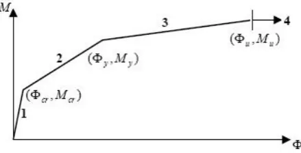
The moment-curvature relation of every Reinforced Concrete (RC) structural element has a definitive effect on the behavior of the structure. In this research the tri-linear moment curvature relation, as shown in Figure 1, is used for expressing the nonlinear behavior of reinforced concrete sections.
various states of behavior of RC elements are used [16,17]:
(a) Cracking state
h y
Nd 6 If
Mcr r (1)
h y
E fr c
cr
(2)
(b) Yielding state
1 β ηn 2 η p η 2βαp
d b 0.5f
My c t 2 0
(3)
1 k
d / cεφy y (4)
(c) Ultimate state
0
y u 1.24 0.15p 0.5n MM (5)
R] S) [(R ε 1.05β
φ 2 0.5
u 1
u (6)
where,
); )d/(1.7f ρf
E ε ρ (
R u s y c S ρεuEsβ1dd/(0.85fc); r
f is the modulus of rupture of concrete; fc is the cylinder strength of concrete; fy is the yield strength of steel;Ec is the modulus of elasticity of concrete; Es is the modulus of elasticity of steel;
u
is the ultimate strain of concrete; y is the yield strain of steel; 1 is a coefficient that depends on the strength of concrete; N is the axial force; d is the depth to rebar; d is the cover depth for compression bars; h is the overall height of section; c is the cover to steel centroid; bt is the top width of section; y is the distance from the
neutral axis of the section to the extreme fiber in tension and is obtained from (7); Iis the moment of inertia of the section and is obtained from Equation 8. Other parameters are defined from Equations 9 to 16.
bt b h t (n 1)(A A )
d A d A 1) (n ) t (h 0.5b t 0.5b y
s s sc b
t
s s sc 2 2 b 2 t
(7)
2
s 2 s sc
2
b 3 b 2 t
3 t
) d (y A y) (d A 1) (n y) 0.5t (0.5h
t h b /12 t) (h b 0.5t) t(y b /12 t b I
(8)
(9)
0.7
0 y y 0
y ε
ε d φ /ε ε 1
0.75
η
(10)
β 1ε ε d φ β 1 α
y y
y
(11)
d /b A ρ d; /b A
ρ s b s b (12)
c y c
y/f ;p ρf /f
f ρ
p (13)
/d d
β (14)
bd N/f
n0 c (15)
0.3 n 0.05 p 0.84
0.45 1.05
c 0
(16)
where nsc is the ratio of the modulus of elasticity of steel to that of concrete; 0is the strain at maximum strength of concrete; bb is the width of the section at the bottom; t is the flange thickness of T or L beam; As is the area of bottom bars and
s
A is the area of top bars. For the case of positive moment, Equations 1 to 16 are valid for all types of sections. For rectangular sections these equations can be simplified by substituting
b b
bb t and t0. Also, for the case of negative
Figure 1. Tri-linear moment curvature curve.
2 2
sc
2
sc
2 2
t t
b b
sc t
b
4α
1 1 1 t
α 2α d
t t
d
b b
d b b
b
t t
d b d
′ ′ ′
p+p + + p − p+p k≤
′ ′
′
− + − −
n (ρ ρ) 1 k>
k= n (ρ+ρ)+ −1 +2n (ρ+ρ β)+ −1
moment, these equations can be used by substituting bt, bb, ht, As and As instead of bb,
t
b , t, As and As, respectively. Ignoring axial effect in beam elements, N, which has been appeared in some above equations, can be considered to be equal to zero. Now by having the moment-curvature relations, the flexural stiffness can be specified for ends of the element as follow:
pm crp crp
p M /φ EI
EI (17)
pm crp
yp crp yp
p (M M )/(φ φ ) EI
EI (18)
pm yp
up yp up
p (M M )/(φ φ ) EI
EI (19)
where Equations 17-19 are used for zones of 1, 2 and 3 of M curve, respectively. In these equations,EIpand EIpm are the stiffness and minimum stiffness of any section; Mcrp, Myp and
up
M are the cracking, yielding and ultimate moments; and crp, yp and up are corresponding curvatures.
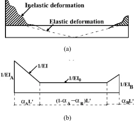
2.2. Material Nonlinearity In this paper, a spread plasticity model that has been proposed by park et al. is utilized [18]. This plasticity model, that considers the cracking behavior of RC, can also consider material nonlinearity of RC elements with a very good approximation. It has been implemented in IDARK software [18]. In this model, for an element subjected to earthquake loading, the distribution of curvature follows Figures 2a,b which is considered for the flexibility distribution in the RC elements, where EIA and
B
EI are the flexural stiffness of the section at end ‘A’ and ‘B’, respectively, and EI0 is the initial stiffness of the element; A and B are the yield penetration coefficients and L is the length of the element.
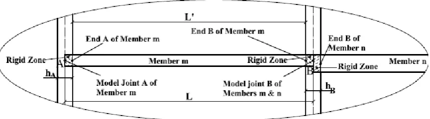
Adopting the above plasticity model for RC elements, the tangent stiffness matrix of each element can be derived. General derivation of tangent stiffness matrix is given by Park et al. [18]. Considering a RC element with six degrees of freedom, with its rigid parts, as shown in Figure 3, the tangent stiffness matrix of element can be
found as follows:
b a
te K K
K (20)
where Ka and Kb are axial stiffness matrix and bending stiffness matrix, respectively and must be assembled in the element stiffness matrixKte. The element stiffness matrix calculated from Equation 20 needs to be transformed to global system:
e te T e
e T K T
K (21)
where Te is the transformation matrix of the element.
a
K can be determined from:
0
1 1
1 1
a
a AK
L EA
K
(22)
where EA/L is the axial stiffness of the element, A is the area of cross section and Ka0 is a constant matrix. Kb, is obtained from the following equation:
T E S E
b R K R
K (23)
(a)
(b)
where:
1
~ ~ ; 1 / 1 0 / 1
0 / 1 1 /
1
K LK L
L L
L L
RTE S S (24)
where L is length of element and L~ can be obtained from the following equation:
B B
A A 1
A B
A B B
A λ 1 λ
λ λ 1 L ; λ 1 λ
λ λ 1 λ λ 1
1
L~ ~
(25) where A and B are the portions of rigid zone at the element ends. The elements of KS in (24) are obtained from the following equation:
b a S11 S22 b c S11 S21 S12
e b B A 0 S11
/f f K K ; /f f K K K
D f L EI EI 12EI K
(26)
where:
L L
L f f f D
S S
S f
S S S f
S S
S f
B A c
b a e
B B A
A c
B B B A
b
B A A A a
) 1
( ;
2 2
2
4 6 4
4 6 4
2 2
3 2 3 3 2 2 1
3 2 3
3 2 1
3 3 3 2 2
1
(27)
where
B A
1 EI EI
S ; S2
EI0EIA
EIB; and
0 B
A3 EI EI EI
S .
The yield penetration parameters used in Equation 27, specify the portion of the element where it cracks. When the moment of the section under consideration is less than cracking moment, the values of these parameters are considered to be equal to zero. For the single curvature of the element, when its moments are greater than cracking moment, the values of the parameters are considered to be equal to 0.5. For other cases, assuming linear moment distribution along the element, these parameters can be determined from:
p crp A B pm
p max min M M M M ,1 ,α
α (28)
where subscript p specifies any general point p and cr represents the cracking state under consideration.
pm is the maximum yield penetration parameter, obtained in previous load steps. Usually, the flexural stiffness at the center of the element is equal to elastic stiffness and is determined from Equation 29. For the case of single curvature if moments are greater than cracking moments, their values can be modified by Equation 30.0 0
0 0 0
2
B A
B A
EI EI
EI EI EI
(29)
B A
B A
EI EI
EI EI EI
2
0 (30)
are the inelastic stiffness at ends ‘A’ and ‘B’, respectively. For a member that yield penetration spreads over the whole element
whenAB 1
,0
EI is obtained from Equation 30. In this case, A
and B and initial flexibility are modified to capture the actual flexibility distribution. These modifications are:
B B A A
B B B A
A f f f f
f f f f
0 0
0
(31)
A
B
1 (32)
A
A AA f f
f
f0 0 / (33)
where:
0 0 1/
; / 1 ; /
1 EI f EI f EI
fA A B B (34)
2.3. Seismic Loading In the pushover analysis, the load vector must incrementally be increased. At each load step, the base shear increment is applied to the structure with a predefined profile over the height of the structure. The incremental lateral load vector can be computed as:
v C b V
ns v c
v cv c
b V E
P .
, 2 ,
1 ,
.
(35)
where Vb is the incremental base shear and Cv is the vector of lateral load distribution factors
s numberof stories
cv,s 1,..., , which is determined
using the following relation [14]:
ns s
ns s
k s H s W
k s H s W s v
c , 1,...,
1
,
(36)
where Ws is the portion of the building seismic weight at story level s; Hs is the vertical distance from base of the building to story level s; ns is the number of stories; and k is a parameter that
has been recommended by FEMA273 as follows [14]:
5 . 2 2
5 . 2 5 . 0 75
. 0 5 . 0
5 . 0 1
T T T
T
k (37)
where T is the fundamental period of the building. 2.4. Nonlinear Responses Since in nonlinear analysis of structure, stiffness isn’t constant and depends on the internal forces of elements and internal forces depend on displacement field, it will be a function of displacement field; on the other hand, displacement depends on stiffness. Then structural analysis is involved in incremental process. The equilibrium equation of the structure is solved using the simple incremental method considering several load steps. No iteration is required within one load step, and thus the numerical algorithm is generally well behaved and exhibits good computational efficiency. In each load step following equation must be solved [19]:
l l l
T u P
K (38)
where l T
K is the tangent stiffness of the structure at load step l; ul is the incremental displacement
vector of the structure at load step land Pl is the
external load vector imposed on the structure at load step l. By having the incremental displacement vector from Equation 38, the displacement vector of the structure at each load step must be updated as follows:
l l
l u u
u 1 (39)
where ul1 and ul are the displacement vector of
the structure at load steps (l1) and (l), respectively. Considering equilibrium of forces for an element, the incremental internal forces of the element at load step
l
can be determined from Equation 40:l e l e l
e K u
F
(40)
where l e
element and ule is the incremental displacement
vector of the element at load step l. By having the incremental internal forces from last mentioned equation, the internal forces of the element at load step l must be updated as follows:
l e l e l
e F F
F 1 (41)
where Fe 1l and Fel are the internal force vectors of the element at load steps (l1) and (l), respectively.
3. NONLINEAR SENSITIVITY ANALYSIS
In the structures undergoing inelastic behavior, incremental methods are usually used to solve equilibrium equation. In this case, displacements are nonlinear function of external loads. Also stiffness is a function of displacements and forces. This causes sensitivity coefficients such as displacement sensitivities to be dependent on stiffness sensitivity, displacement sensitivity, external load sensitivity and internal load sensitivity; while in linear structures, they only depend on stiffness sensitivity and external load sensitivity. Finding sensitivity relations in nonlinear structures is too difficult for this complicacy; on the other hand, applying linear sensitivity theory leads to incorrect results. In the present study, to drive relations for nonlinear sensitivities, equilibrium equations are differentiated at each load step. This is explained in the next section.
3.1. Displacement Sensitivity Considering incremental Equation 38 and differentiating it with respect to design variablexj, we get to:
j l
j l l T l j l T
dx P d dx
u d K u dx
dK (42)
where l T
K is the global tangent stiffness matrix;
l
u
is the incremental displacement vector;
j l T
dx dK
is the sensitivity of the global tangent stiffness
matrix;
j l
dx u
d is the sensitivity of the incremental
displacement vector and
j l
dx P d
is the sensitivity of the incremental external load vector at load step l
with respect to design variablexj. In this study, Equation 42 is used as the basic formulation for obtaining the incremental displacement sensitivities. Assuming that all terms in Equation 42 except
j l
dx u d
are known, it will be rearranged to find:
l
j l T j
l l
T j
l
u dx dK dx
P d K dx
u
d 1
(43)
The total sensitivity of displacement vector can be obtained by summing up the sensitivities in all load steps as follows:
j l
j l
j l
dx u d dx du dx
du 1
(44)
where
j l
dx
du1 and
j l
dx
du are the sensitivities of the incremental displacement vector at load steps
) 1
(l and (l), respectively. The term
j l
dx u
d is the sensitivity of the incremental displacement vector which is obtained from Equation 43. For this, sensitivities of stiffness and external loads need to be determined. In the coming sections, the way each sensitivity item in Equation 43 should be obtained, is explained.
3.1.1. Sensitivity of stiffness The tangent stiffness matrix of the structure at each load step is obtained by properly assembling of the tangent stiffness matrix of elements:
ne
e e l
T K
K
1
(45)
where ne is the number of structural elements and
e
45 with respect to any generalized variable, xj, sensitivity of the tangent stiffness matrix can be obtained from:
ne e j e j l T dx dK dx dK 1 ) ( (46)Based on the last equation, to compute tangent stiffness sensitivity, it is sufficient to calculate sensitivity of tangent stiffness of all elements. Sensitivity of tangent stiffness matrix of each element is obtained by differentiating from Equation 21: e j te T e j e T dx dK T dx dK (47)
In the above equation,
j te
dx
dK is the sensitivity of the tangent stiffness matrix of the element including axial effects sensitivity and bending effects sensitivity in local system and can be obtained by differentiating from Equation 20:
j b j a j te dx dK dx dK dx
dK (48)
It is noted that the first and second terms in the right hand side of Equation 48 must be properly assembled. The first term represents the axial stiffness while the second one represents flexural stiffness. These two sensitivity matrix are obtained by differentiating Equations 22 and 23 noting that matrices of K a 0 and R E utilized in these equations are independent of design variables and can be determined as follow:
0 a j j a K dx dA dx dK (49) T E j S E j b R dx dK R dx
dK (50)
Assuming rigid diaphragm for floors, there will be no change in axial forces of beams. Accordingly, the axial stiffness sensitivity for beams is zero. For column elements by definingAbh, the sensitivity of A with respect to b ish, and with respect to h isb. It is zero with respect to other variables. The
sensitivity of matrix KS utilized in Equation 50 is determined by differentiating from Equation 24:
j S j S S j j S dx L d K L L dx K d L L K dx L d dx
dK ~ ~1 ~ ~1 ~ ~1 (51)
where: j B j B j A j A j j A j B j A j B j B j A B A j dx d dx d dx d dx d dx L d dx d dx d dx d dx d L dx d dx d dx L d 1 ~ ~ 1 1 ~ (52)
In Equation 52, sensitivity of A with respect to
A
h is1/2L; also sensitivity of B with respect to
B
h is1/2L. For a typical beam hA and hB have been shown in Figure 3. Similar definitions can be made for columns between two floor beams. In Equation 51 sensitivities of matrix KS with respect to any design variable can be obtained by differentiation of its elements as follow:
e b j e b j j b e B A A j B B j A B A j e b j S D f L dx dD f dx L d L dx df D EI EI EI EI EI dx dEI EI EI dx dEI EI EI dx dEI D L f dx dK 0 0 0 0 11 12 12 (53) 211 11 11 12 b S c j b b S j c b c j S j S f K f dx df f K dx df f f dx dK dx
dK (54)
2 11 11 11 22 b S a j b b S j a b a j S j S f K f dx df f K dx df f f dx dK dx
dK (55)
1 3 2 2 3 2 2 3 2 3 4 3 8 6 3 4 6 S S dx d S dx d S S dx df A j B B B j A A B B B j b (57)
1 2 3 3 2 3 2 2 3 2 2 2 3 4 2 3 4 2 S dx d S S dx d S S dx df j B B B B B j A A A A A j c (58)
j c b a j c c a j b b j a j e dx L d L f f f L dx df f f dx df f dx df dx dD 2 2 2 2 (59) L dx d dx d dx L d j b j a j (60) where:
j A B A j B j j B A B j A j A j B B j A dx dEI EI EI EI dx dEI dx dEI S dx dEI EI EI EI dx dEI dx dEI S EI dx dEI EI dx dEI S 0 0 3 0 0 2 1 (61)In these equations, the derivative of EI0 with respect to any variable X can be obtained by differentiating from Equation 29 with respect to X. This leads to Equation 62:
j B j A B A B A A j B B j A B A j dx dEI dx dEI EI EI EI EI EI dx dEI EI dx dEI EI EI dx dEI 0 0 2 0 0 0 0 0 0 0 0 0 0 0 ) ( 2 2 (62)
For an element with two end moments greater than cracking moment and single curvature, the sensitivity of EI0 with respect to X should be
modified by Equation 63. Sensitivity of EIA0 and
0
B
EI will be obtained from Equation 64
considering the case ofMp Mcrp:
j B j A B A B A A j B B j A B A j dx dEI dx dEI EI EI EI EI EI dx dEI EI dx dEI EI EI dx dEI 2 0 ) ( 2 2 (63)
In Equations 53 and 61 to 63, to use the sensitivity
A
EI andEIB, it is sufficient to differentiate Equations 17 to 19 with respect to xjas follow:
j crp crp crp j crp crp j p dx d M dx dM dx dEI 2 1 (64) j crp j yp crp yp crp yp j crp j yp crp yp j p dx d dx d M M dx dM dx dM dx dEI 2 ) ( 1 (65) j yp j up yp up yp up j yp j up yp up j p dx d dx d M M dx dM dx dM dx dEI 2 ) ( 1 (66)
where Equations 64, 65 and 66 are used for zones of 1, 2 and 3 of M curve, respectively.
determined by differentiating from Equation 28: j B j A B A crp p j crp p p j p B A j p dx dM dx dM M M M M dx dM M M dx dM M M dx d ) ( 1 (67)
where dMp/dxjis the sensitivity of moment at end 'p' of the element; its value will be presented in section 3.3. In Equation 67, if p>1, its sensitivity is zero and if p<pm, its sensitivity is equal to sensitivity of pm. When AB1, the sensitivity of EI0, A and B must be modified by differentiation of Equations 31 to 33:
2 0 0 0 2 0 0 2 0 0 0 0 2 0 0 B B A A B B B A B B j B B x Bx A A j A A x Ax B B A A B B j B B x Bx Bx Ax j A f f f f f f f f f f dx d f f f f dx d f f f f f f f f dx d f f f f dx d (68) j A j B dx d dx
d (69)
j A A A j A A A A A x Ax Ax j dx d dx d f f f f f dx f d 2 0 0 0 1 ) ( (70) where: 2 0 0 0 2 2 1 ; 1 ; 1 EI dx dEI f EI dx dEI f EI dx dEI f j x B j B Bx A j A
Ax (71)
3.1.2. Sensitivity of loads Since seismic loads depend on the natural period of the structure and the natural period depends on structural stiffness and building mass, any change in the structure
stiffness causes a change in the external loads. Since gravity loads are constant, the sensitivity of external load vector at any load step l comprises only sensitivity of lateral loads.
j E j l E j l dx P d dx dP dx
dP 1
(72)
where the second term in right hand side is the sensitivity of incremental seismic loads and is obtained from j v b j E dx dC V dx P d . (73)
where the components of dCv/dxj vector are found from the following equation:
j ns s k s s s n ns s k s s s n ns s k s s k s s j s v dx dk H W H l H W H l H W H W dx dc
1 1 1 , (74)In the above equation, for T0.5 and T2.5, the sensitivity of k is zero. For other values of T, derivative of Equation 37 gives:
j j 0.5dT/dx
dk/dx (75)
where dT/dxj is the sensitivity of the fundamental period of the structure and can be found from the following relation [20]:
dx dK 8 T -= dx dT j T 2 3 j (76)
where
is the first mode shape of the structure. 3.2. Force Sensitivity Since in nonlinear structures, displacement is an implicit function of internal forces; force sensitivities need to be calculated for computation of displacement sensitivity. Sensitivity of the incremental internal forces of any typical element at load step l can be determined by differentiating from Equation 40:The sensitivity of internal forces of the element is updated by Equation 78:
j l e j 1 l e j l e dx ΔF d dx dF dx
dF (78)
where
j l e
dx
dF 1 is the sensitivity vector of internal
forces at previous load step and
j l e dx F d
is the sensitivity vector of incremental internal forces determined from Equation 77. Components of the sensitivity vector, which is obtained by Equation 78, give sensitivity of forces such as moment sensitivity and axial force sensitivity which are appeared in some sensitivity equations derived in previous sections.
3.3. Moment-Curvature Curve Sensitivity Since moment-curvature relations are functions of design variables and axial forces and sensitivity equations derived in previous sections are dependent on their sensitivities, these sensitivities including cracking moment sensitivity, yielding moment sensitivity, ultimate moment sensitivity, cracking curvature sensitivity, yielding curvature sensitivity and ultimate curvature sensitivity need to be determined. These sensitivities at each load step are variable for existence of axial forces. This causes that nonlinear sensitivity analysis be more difficult than the state in which, sensitivity of axial loads is ignored. Sensitivities of moment-curvature characteristics can be obtained by differentiating from Equations 1 to 6 at various states:
(a) Cracking state
6 ) d(dN/dx 6 ) N(dd/dx y) (h ) dy/dx I(dh/dx f dy/dx dh/dx ) (dI/dx f dx dM j j 2 j j r j j j r j cr (79)
2 c j j r j cr y h E dh/dx dy/dx f dx dφ ( ) (80)
(b) Yielding state
j j j j j j 0 j j j 0 2 c 0 j 2 j c j y dx dα p dx p d α 2β η p α dx dβ 2 dx dη dx dη p dx dp η 2 n dx dη dx dβ dx dn η β 1 d b 0.5f p α 2β η p η 2 n η β 1 dx dd d 2b d dx db 0.5f dx dM (81) y j j j j y d k c k dx dd dc dx dk d k dx dc dx d 2 2 ) 1 ( ) 1 )( / ( ) / ( ) 1 )( / ( (82) (c) Ultimate state
yj j j y j u M dx dn dx dp dx dM n p dx dM 0
0 0.15 0.5
5 . 0 15 . 0 24 . 1 (83)
uj j j j j u R S R dx dR S R dx dS dx dR R c dx dc R S R dx d 1 2 5 . 0 2 5 . 0 2 5 . 0 2 ) ( ) ( 2 5 . 0 ) ( (84) In above equations, unknown sensitivities are obtained by differentiating from Equations 7 to 16 and R aqnd S (the extended form should be used) equations with respect to design variable xj from
the following equations:
j y j y y y y j dx dh dx d d d dxd
7 . 0 0 0 3 . 0 ) / 1 ( 525 . 0 (86)
j dx d j dx dh y j dx y d d y y y d y j dx d j dxd
1 (87)
d t k j dx dh 2 d t j dx dt d 1 1 b b t b j dx b db 2 b b t b j dx t db b b 1 d t j dx ρ d j dx dρ sc n j dx dh 3 d 2 t j dx dt 2 d t 1 b b t b 2 j dx b db 2 b b t b j dx t db b b 1 2 d 2 t j dx dβ j dx ρ d ρ β j dx dρ sc 2n j dx dh 2 d t j dx dt d 1 1 b b t b j dx b db 2 b b t b j dx t db b b 1 d t j dx ρ d j dx dρ sc n 1 b b t b d t ) ρ (ρ sc 2n 0.5 2 d 2 t 1 b b t b sc 2n β ρ ρ 2 1 b b t b d t ) ρ (ρ sc n 0.5 d t k j dx p d j dx dp 2α 1 j dx dα 2 2α p p 2 α p β p j dx dα j dx p d β p j dx dβ j dx dp α 1 j dx dα 3 2α 2 ) p (p 2 2α p p j dx p d j dx dp 0.5 α p β p 2 2α p p 2 1 j dx dk (88)
c s A d s A 1 sc n b 0.5b 2 t 2 h 2 t t 0.5b j dx s A d j dx s dA 1 sc n j dx dh b b t h j dx b db j dx dt t b t j dx t db s A s A 1 sc n t t b t h b b d j dx s A d j dx dh s A d j dx s dA 1 sc n j dx dt t j dx dh h b b 2 t 2 h j dx b db 0.5 j dx dt t t b 2 t j dx t db 0.5 2 c s A d s A 1 sc n 2 t 2 h b 0.5b 2 t t 0.5b 1 j dx dy (89) j b j b b s j s b j dx dh b d dx db d b A dx dA d b dx d 2 2 1 (90) j b j b b s j s b j dx dh b d dx db d b A dx A d d b dx d 2 2 1 (91) j c y j dx d f f dxdp (92)
j c y j dx d f f dx p
d
(93) j 2 j dx dh d d dx
dβ (94)
j jj dx dn p dx dp p n dx dc 0 2 0 3 . 0 1 05 . 0 84 . 0 45 . 0 84 . 0 5 . 1 (95) j j c j c j dx dh b d dx db d b f N dx dN bd f dx dn 2 2
0 1 (96)
j y s u y j s u j c j dx dh f E d f dx d E dx d f dx dR ) ( 7 . 1
j j
c s u
j dx
dh d dx d f
d E dx
dS
85 . 0
1 (98)
In equations presented in this section, values of
j t
dx db ,
j b
dx db ,
j
dx dt and
j
dx
dh are equal to 1 for t
b b
xj t, b, and h, respectively. Values of these parameters for other design variables are equal to zero. Axial load sensitivity
j
dx
dN that exists in some equations is one component of sensitivity vector obtained from section 3.2.
3.4. Summary of Sensitivity Analysis Procedure
The nonlinear sensitivity analysis of RC frames that was developed in this study can be carried out in the following steps:
1. Compute the first mode shape, first period and its sensitivity from Equation 76
2. Calculate the matrixes L~ and L~1 and their derivatives for each element from Equations 25 and 52
3. Compute the lateral load distribution factors and their sensitivities by Equations 36 and 74
4 Set load step index l1 and apply the gravity loads only
5. Determine the moment-curvature relations from Equations 1 to 6 and compute their derivatives from section 3.3
6. Compute the lateral loads and their sensitivities from Equations 35 and 73 7. Compute the flexural stiffness and yield
penetration parameters and their sensitivities for each element from Equations 17 to 19 and Equations 64 to 66
8. Compute the yield penetration parameters and their sensitivities for each element from Equations 28, 31, 32, and Equations 67 to 69 9. Compute the tangent stiffness matrix and its
sensitivity for each element by Equations 21 and 47
10. Assemble the global tangent stiffness matrix and its matrix of sensitivity by Equations 45 and 46
11. Solve Equation 38 for displacements and find their incremental sensitivities from Equation 43
12. Calculate the internal forces and their sensitivities from Equations 40 and 77 13. Set ll1, if the roof lateral displacement
is greater than target displacement, stop the sensitivity analysis and go to step 14; otherwise go to step 5.
14. Compute the total incremental sensitivities coefficients
4. NUMERICAL EXAMPLE
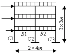
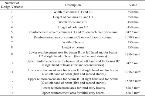
A three-story, two-bay planar frame of Figure 4 is used to illustrate the method of proposed analytical nonlinear sensitivity analysis. The concrete is assumed to have a cylinder strength of 30 MPa, a modulus of rupture of 3.45 MPa, a modulus of elasticity of 27,400 MPa, a strain of 0.002 (unit?) at maximum strength and an ultimate strain of 0.003. The steel has yield strength of 300 MPa and a modulus of elasticity of 200,000 MPa. A uniformly distributed gravity load of 12 KN/m is applied on the beams of each story. Reinforcements have the cover to the steel centroid of 50 mm. It is assumed that columns and beams have rectangular cross sections. Fourteen design variables which have been given in Table 1 are defined in this frame. In order to allow the structure to enter to the inelastic behavior, target displacement of 2% has been chosen as a stop criterion for load steps of sensitivity analysis. The pushover (capacity) curve of this frame is shown in Figure 5 and target point has specified on it for two cases namely (i) flexural effect only, C0 and (ii) both flexural and axial effects, C1. Nonlinear sensitivity analysis is performed on this frame by the proposed Analytical Method (AM)
for cases of (i) and (ii) and compared to the results from central Finite Difference Method (FDM). As a sample, sensitivity analysis of the overall drift that may indirectly represent the sensitivity of internal forces to change in some design variables is considered. The results have been briefed in Table 2. For interpreting the results, for example, consider the design variable No.7. The overall drift sensitivity shows that its value will be decreased by 1.1499% and -1.3875% for a unit change in the design variable No.7 for cases i and ii, respectively. Values of nonlinear sensitivity coefficients predict that if the value of width of beams increases from 250mm to 260mm; overall drift decreases 2% to 1.9885% and 1.9861% for C0 and C1, respectively. This prediction is very important in optimal performance-based design process. Sensitivity results for cases (i) and (ii) show that sensitivity coefficients of C0 and C1 are
not the same. This difference is considerable for some design variables such as variable No.1. Therefore, existence of axial forces can affect sensitivity coefficients with respect to the design variables. For the present example, it is observed that the values of sensitivity coefficients of C1 are smaller than those of C0 for most of design variables. That is existence of axial loads decreases the displacement sensitivity in most of cases. In Table 2, percentage of error of FDM compared to AM has been evaluated from:
SFDM SAM
SAMERROR100 / (99)
In Equation 99, SFDM and SAM are the sensitivity
coefficients obtained from FDM and AM, respectively. In the FDM method, the design variables perturbation has been considered to be 1% and 0.001%. Comparing the AM results with
TABLE 1. Design variables.
Number of
Design Variable Description Value
1 Width of columns C1 and C3 350 mm
2 Height of columns C1 and C3 350 mm
3 Width of columns C2 450 mm
4 Height of columns C2 450 mm
5 Reinforcement area of columns C1 and C3 on each face of column 942.5 mm² 6 Reinforcement area of columns C2 on each face of column 1570.8 mm²
7 Width of beams 250 mm
8 Height of beams 350 mm
9 Lower reinforcement area for beams B1 at left hand and for beams
B2 at right hand of beam (first and second stories) 1256.6 mm² 10 Upper reinforcement area for beams B1 at left hand and for beams B2
at right hand of beam (first and second stories) 942.5 mm² 11 Lower reinforcement area for beams B1 at right hand and for beams
B2 at left hand of beam (first and second stories) 1256.6 mm² 12 Upper reinforcement area for beams B1 at right hand and for beams
B2 at left hand of beam (first and second stories) 1570.8 mm²
13 Lower reinforcement area for third story beams 628.3 mm²
that of FDM shows that by reducing perturbation values from 1% to 0.001% results of FDM for almost all design variables converge to AM results; that is, the AM results are in a good agreement with FDM results in very small perturbation cases. This matter verifies the AM results.
The results of sensitivity analysis by FDM shows
that assuming perturbation of 1% in design variables, this method in all cases generates inaccurate results; while this is not the case in the linear sensitivity analysis. On the other hand, considering small perturbations for some design variables may lead to run-time errors. Hence, the proposed method can efficiently reduce errors of FDM.
Figure 5. Capacity curve of the three-story RCMRF.
TABLE 2. Sensitivity Coefficients of Overall drift at Target Point (%).
Method Sensitivity with Respect to Design Variable
1 4 5 7 8 9 12
AM C0 -0.2688 -10.8864 -3284.1 -1.1499 -46.3542 -2333.1 -2183.6
C1 -0.0064 -7.9053 -1642.1 -1.3875 -41.7281 -1988.7 -1993.5 FDM 1% C0 -0.4757 -10.6962 -3171.2 -1.7722 -61.3068 -2140.8 -2548.7 C1 -2.7673 -9.5303 -2128.5 -0.0931 -56.8434 -3020.5 -3106.0 FDM 0.001% C0 -0.2688 -10.8859 -3284.1 -1.1499 -46.3487 -2332.9 -2183.3 C1 -0.0064 -7.9054 -1641.9 -1.3871 -41.7283 -1988.6 -1993.4
ERROR 1% C0 76.95 -1.75 -3.44 54.12 32.26 -8.24 16.72
C1 42873 20.55 29.62 93.29 36.22 51.88 55.80
ERROR 0.001% C0 -0.03 -0.005 -0.001 -0.001 -0.01 -0.006 -0.01
5. CONCLUSION
In the present study a procedure for exact nonlinear sensitivity analysis of RCMRF was proposed. The procedure includes both flexural and axial effects in the context of pushover analysis. The proposed sensitivity method does not face the difficulties that the FDM method confronts and can reduce errors of FDM.
Sensitivity analysis of a three-story RC frame illustrated the capability and effectiveness of the derived formulations. It was shown that existence of axial forces can affect sensitivity coefficients with respect to the design variables. Results of the case study for a nonlinear structure indicate that sensitivity calculation via FDM method may end up to inaccurate sensitivity results especially if the value of perturbation is high.
6. REFERENCES
1. Ryu, Y.S, Haririan, M., Wu, C.C., and Arora, J.S., “Structural design sensitivity analysis of nonlinear response”, Computers and Structures,Vol. 21, (1985), 245-255.
2. Choi, K.K., and Santos, J.L.T., “Design sensitivity analysis of nonlinear structural systems Part I: Theory”, International Journal for Numerical Methods in Engineering,Vol. 24, (1987), 2039-2055.
3. Gopalakrishna, H.S., and Greimann, F., “Newton-Raphson procedure for the sensitivity analysis of nonlinear structural behavior”, Computers and Structures, Vol. 30, (1988), 1263-1273.
4. Santos, J.L.T, and Choi, K.K., “Shape design sensitivity analysis of nonlinear structural systems”, Structural and Multidisciplinary Optimization, Vol. 4, (1992), 23-35.
5. Ohsaki, M., and Arora, J.S., “Design sensitivity analysis of elasto-plastic structures”, International Journal for Numerical Methods in Engineering, Vol. 37, (1994), 737-762.
6. Lee, T.H., and Arora, J.S., “A computational method for design sensitivity analysis of elastoplastic Structures”, Computer Methods in Applied Mechanics and Engineering, Vol. 122, (1995), 27-50.
7. Barthold, F.J., and Stein, E., “A continuum mechanical-based formulation of the variational sensitivity analysis in structural optimization Part I: Analysis”, Structural and Multidisciplinary Optimization, Vol. 11, (1996), 29-42.
8. Szewczyk, Z.P., and Ahmed, K.N., “A hybrid numerical/-neurocomputing strategy for sensitivity analysis of non-linear structures”, Computers and Structures, Vol. 65, (1997), 869-880.
9. Yamazaki, K., “Sensitivity analysis of nonlinear material and its application to shape optimization”, AIAA Journal, Vol. 36, (1998), 1113-1115.
10. Bugeda, G., Gil, L., and Onate, E., “Structural shape sensitivity analysis for nonlinear material models with strain softening”, Structural and Multidisciplinary Optimization, Vol. 17, (1999), 162-171.
11. Schwarz, S., and Ramm, E., “Sensitivity analysis and optimization for nonlinear structural response”, Engineering Computations, Vol. 18, (2001), 610. 12. Gong, Y., Xu, L., and Grierson, D.E., “Sensitivity
analysis of steel moment frames accounting for geometric and material nonlinearity”, Computers and Structures, Vol. 84, (2006), 462-475.
13. Habibi, A.R., and Moharrami, H., “Nonlinear Sensitivity Analysis of Reinforced Concrete Frames”, Finite Elements in Analysis and Design, Vol. 46, (2010), 571-584.
14. FEMA-273, “NEHRP Guideline for the seismic rehabilitation of buildings”, Federal Emergency Management Agency, Washington, DC, U.S.A., (1997). 15. ATC-40, “Seismic evaluation and retrofit of concrete
buildings”, Applied Technology Council, California Seismic Safety Commission, U.S.A., (1997).
16. Park, R., and Paulay, T., “Reinforced concrete structures”, John Wiley and Sons, Inc., New York, U.S.A., (1974).
17. Park, Y.J., and Ang A.H.S., “Mechanistic seismic damage model for reinforced concrete”, Journal of Structural Engineering, ASCE, Vol. 111, (1985), 722-739.
18. Park, Y.J., Reinhorn, A.M., and Kunnath, S.K., “IDARC: Inelastic damage analysis of frame shear-wall Structures”, Technical report NCEER-87-0008, National center for earthquake engi