A Hybrid Dynamic Programming for Inventory Routing Problem in Collaborative Reverse Supply Chains

Please cite this article as: N. S. Tabrizi, M. Yavari, Adsorption of Methylene Blue from Aqueous Solutions by Silk Cocoon, International Journal of Engineering (IJE), TRANSACTIONS A: Basics Vol. 29, No. 10, (October 2016) 1412-1420

International Journal of Engineering

J o u r n a l H o m e p a g e : w w w . i j e . i r

A Hybrid Dynamic Programming for Inventory Routing Problem in Collaborative

Reverse Supply Chains

M. Moubeda_{, Y. Zare Mehrjerdi}*b

a _{Department of Industrial Engineering, Faculty of Engineering, Ardakan University} b _{Department of Industrial Engineering, Faculty of Engineering, Yazd University}

P A P E R I N F O

Paper history: Received 21 April 2015

Received in revised form 09 August 2016 Accepted 25 August 2016

Keywords: Reverse Supply Chains Collaboration Dynamic Programming Ant Colony Optimization Tabu Search

A B S T R A C T

Inventory routing problems arise as simultaneous decisions in inventory and routing optimization. In the present study, vendor managed inventory is proposed as a collaborative model for reverse supply chains and the optimization problem is modeled in terms of an inventory routing problem. The studied reverse supply chains include several return generators and recovery centers and one collection center. Since the mathematical model is an NP-hard one, finding the exact solution is time consuming and complex. A hybrid heuristic model combining dynamic programming, ant colony optimization and tabu search has been proposed to solve the problem. To confirm the performance of proposed model, solutions are compared with three previous researches. The comparison reveals that the method can significantly decrease costs and solution times. To determine the ant colony parameters, four factors and three levels are selected and the optimized values of parameters are defined by design of experiments.

doi: 10.5829/idosi.ije.2016.29.10a.12

1. INTRODUCTION1

Reverse supply chain consists of a series of activities needed to retrieve a used product from the point of use and either dispose or recover its value. By increasing level of consumption, waste and public awareness about environmental problems, the significance of the reverse supply chains has been quickly identified in academic and business world. Several studies have been conducted in different fields of these chains. However, the great implementation costs as stated by some supply chain members and references [1, 2], caused these chains to work slower in application than theory. Collaboration is an approach to reduce the primary costs and can be employed as a method to make these projects as economic ones. In the present study, a model is proposed to collaborate between components of parallel reverse chains that try to minimize total costs of chains. The costs involve ordering, holding, transportation, loading, unloading costs and penalties for not using raw

1_{*Corresponding Author’s Email:}

[email protected] (Y. Zare

Mehrjerdi)

materials and disposing in non-environmentally friendly ways.

2. LITERATURE REVIEW

Supply Chain Collaboration (SCC) has received great attention in recent years as a key success factor for leaders [3, 4]. Reviewing the SCC literature in 2014 shows that the most talked benefits are cost saving, inventory reduction, visibility increase and reduction in bullwhip effect [5]. Hernández et al. defined SCC as a way that the members of a supply chain actively work together and share their information, risks, knowledge and profits [6]. Content analysis of literature between 1997 and 2006 have shown that the main concentration of previous works were on vertical collaboration between organizations and its suppliers or customers and vertical collaboration is ignored [7]. In another investigation, Hudnurkara et al. [5] identified 28 factors affecting SCC, that information sharing is the most highly talked one.

studied widely. Setak and Daneshfar [8] by reviewing the literature demonstrated that before the second half of 90thVMI was considered just as a flavoring item. By new and update information and communication technology and demand transparency between chain members, it becomes possible to optimize the inventory management for all members. So, the inventory decreases along with the decrease in bullwhip effect. As a result, the required space and various costs of chains will decrease. VMI results in better planning and modification of production and distribution, improving services, better availability of data and improved communication with customers. This system is an automatic integrated replenishment which results in lower costs and higher ability of clients for emphasizing on their competitive advantages [8, 9].

In collaborative reverse supply chains, some researchers paid special attention to the role of communication and others consider the decision support systems and information systems as tools for it [10]. One of the first papers in reverse supply chains, by Zhang and Sun [1], introduced cooperation and synchronization of reverse supply chain partners as a success factor for them. They defined opportunities for cooperation in the processes for waranny, return material authorization, return price rationalization and product returns with damaged packaging. Bai [11] developed a model for collaboration between customers, retailers and producers in order to maximize the return of ink cartridge. In this structure, the OEM and 3rd party refiller collaborate. To examine the impact of this new structure, the results and cost functions are compared with the previous structure and it is found that in the new model returns will increase; all stakeholders concentrate on their own capabilities and costs will reduce. Lambert et al. [12] added integrated information system as a component to the usual framework of open-loop reverse supply chains. This system is known as most important part of model which establishes a relationship between different components of reverse supply chain.

Aras et al. [13] using a heuristic algorithm and tabu search (TS) solved a VRP for planning the collection of durable goods from dealers. They studied the case that a firm wants to collect cores from the dealers and return to the collection center (CC). These dealers charge the company for the collected products. Therefore, the returns can only be taken back if the acquisition price exceeds the dealer charges. A comparison between the report available in the literature [13] and our problem shows that collection is not obliged for every center and just takes place in special conditions.

Le Blanc [2] developed a concept called Collector Managed Inventory (CMI) as a variant for VMI in reverse supply chain. In this system, two levels of inventories: can order (CO) and must order (MO) are introduced.

When inventory reaches MO, collecting trucks must go towards the point and collect returns. CO is the inventory level that is used to profitably fill up the remaining capacity of trucks, but cannot start a collection. Gou et al. [14] developed the previous methods, proposed a new policy for inventory management in open-loop chains. They defined optimal economic parameters to minimize the total system costs. Joint inventory management was introduced by these researchers later and a method was defined for inventory management in central and local collection points. This study minimizes the average long-term costs of chain [15]. However, the study focus is on inventory and not optimizing the routes. Developing [2, 15], a comprehensive model will be provided for managing inventories and routing in the current paper.

By developing VMI, Inventory Routing Problems (IRP) become more significant, since the supplier must make three decisions simultaneously: (a) When should the company send the product to customers? (b) How many products should be sent? (c) Which is the optimal route [16]? Coelho et al. investigated IRP by considering transshipment that means goods can be shipped to a customer either directly from the supplier or from another customer. Large neighborhood search heuristic is used to determine the routes and network flow algorithm to specify the delivery quantities and transshipment moves [17]. In an IRP problem with backlogging, a meta-heuristic method is developed based on parallel genetic algorithms to solve MINLP (mixed integer nonlinear programming). The proposed solutions and previous methods are compared to confirm its performance [18]. Mirzaei et al. [19] studied inventory, production and distribution planning in a two-echelon supply chain with one producer and several retailers in a multi-period, multi-product case. A two-step algorithm including Particle Swarm Optimization (PSO) and linear programming is proposed to solve the problem.

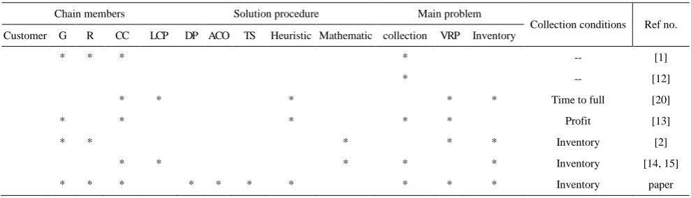
TABLE 1. The relevant literature

Chain members Solution procedure Main problem

Collection conditions Ref no. Customer G R CC LCP DP ACO TS Heuristic Mathematic collection VRP Inventory

* * * * -- [1]

* -- [12]

* * * * * Time to full [20]

* * * * * Profit [13]

* * * * * Inventory [2]

* * * * * Inventory [14, 15]

* * * * * * * * * * Inventory paper

3. PROBLEM DEFINITION

As described earlier, IRP in reverse supply chain is more complex because of aspects such as non-deterministic return production and consumption. We focus on open-loop reverse supply chains, which include the following members and echelons:

 Return Generators (G): Places where returns are produced, gathered or held. They can be wholesalers or retailers who gather customers' returns or manufacturers who hold their scraps to send for recovery centers. If collection does not take place, scraps will be disposed.

 Recovery centers (R): Various options are introduced for returns in a reverse supply chain that differ according to product features, its life cycle phase and other characteristics. These options may be reuse, resale, repair, remanufacture, refurbish and recycle. In order to be applicable for all options, we use the word "recovery" that is more common and can be each of these options.

 CC as an intermediate center is responsible for collecting, holding and transferring returns.

In the non-collaborative case, each chain works in isolation and plans its own collection and delivery of returns that will increase total costs. Our problem is to plan for return collection and delivery, in the case that all members collaborate. Multiple Gs, Rs and one CC are assumed. CC has information about members' inventory levels and plans the vehicle routes to decrease whole supply chain costs. CC also can hold returns for some time when there is no place in any Rs to accept them.

One of the early collaboration types in reverse supply chains is using central collection point for sorting, reprocessing and transferring returns as shown by researchers [15, 21]. Advantages such as better inventory turnover, information visibility, finding more quality problems, decreasing inventory levels and related costs are demonstrated for these centers [22].

4. THE PROPOSED MODEL

4. 1. The Collaborative Process The proposed

model is designed in accordance with VMI in forward supply chains. CC has the information about inventory levels of Rs and Gs and plans for collecting and transferring returns through the chains. These plans must minimize the whole supply chain costs for multi-period case. A route will start only when a G reaches its MP or a R reaches its order point (OP). The following summarizes the main assumptions of this paper:

The model is a multi-period one.

Number of Gs and Rs is known and fixed.

Holding, shortage, transportation and disposal penalty costs are known for each location.

Holding cost depends on mean inventory level. Stock-out cost depends on its quantity and time. Gs' Returns cannot be collected before reaching CP. The routes start and finish must be at CC.

Trucks and their capacities are similar.

Lead time is zero, returns will be delivered by Rs at the same period that are collected.

When a G's inventory exceeds MP, it cannot hold returns more than CP and will dispose them.

CP is zero for CC, means that when there is some inventory in CC, it can be inserted in a route. MP is unlimited for CC because it can warehouse.

The inventory capacity of Rs is limited. Rs just when reach their OP, can deliver returns.

MP is unlimited for CC.

4. 2. Model Formulation The notations for

mathematical formulation are: Time period (t = 1,2,...,T) t

Number of Gs and Rs n,m

Nodes (1,2,...,n for Gs, n+1 for CC and n+2,...,n+m+1 for Rs)

i,j

Parameters:

Production rate in Gi at period t t

i SP

Return demand rate at Ri at period t

t i D

The economic order quantity for Ri

i EO

Reorder point for Ri i

E

Distance between i and j

ij d

Returns holding cost at G, C and R

Rh Ch

Gh C C

C , ,

Loading and unloading cost

U

L C

C ,

Transportation cost per kilometer

m C

Route / truck start cost

S C

Stock-out cost for each Ri

SO C

Penalty cost for disposal

P

C

Truck capacity (assumed the same for all) TP

Variables:

Amount of returns collected at Gi in period t t

Gi Q

Amount of returns delivered to Ri in period t t

Ri Q

Amount of returns at CC in period t

t C Q

Stock-out amount at Ri at period t t

i SO

If Gi inventory reaches MP at t = 1 else = 0 t

i x

If Gi inventory reaches CP at t = 1 else = 0 t

i y

If Rireaches it OP at period t = 1 else =0 t

i O

Remain truck capacity at kth stop of period t

t K RTP

Decision variables:

Number of trucks start their route at period t

t f

Truck goes from i to j at period t = 1

t ij

Z

Scraps picked from i at period t = 1 i=1,…n

t i

b

Returns loaded at Gi in kth stop of period t

t ik

QL

Scraps unloaded in i at period t = 1 ,i=n,…n+m

t i

a

Returns unloaded in Ri at kth stop of period t

t ik

QU

The model objective is to collect most possible returns from Gs while minimizing costs. The objective function (1) consists of holding cost for returns at Gs, Rs and CC, transportation, stock-out for Rs, loading and unloading, start for each tour, and penalty for not-covering Gs.





 



  

  



 









                                  T t n i t i i t C t i P T t t S T t n i kk k t ik L T t m n n i kk k t ik U T t t i SO T t m n j i ij t ij m T t t C Ch m n n i t Ri Rh n i t Gi Gh b CP Q x C f C QL C QU C SO C d Z C Q C Q C Q C Min 1 1 1

1 ,1 1 1 1 1 , 1 1 1 1 1 , 1 T 1 t 1 2 1 ) 1 )( ( Z (1)

Consriants are defined in three main categories:

A) Load/Unload Quantity

Costraints (2) and (3) impose maximal for QL; that is the minimum of remained truck capcaity and returns Inventory level at Gs. Also (4) shows that quantity of returns loaded at G must be greater than the CP of that center. For the CC, this amount can not exceed the quantity of returns collected at that center (5). Equation

(6) shows that the unloaded amount at each stop must be less than the collected amount in the truck before that stop. The two next consriants (7) and (8) assure that the unload quantity at Rs at each stop is less than the center's Economic Order Quantity (EOQ) and more than its OP. These equations are used to avoid stock-out at Rs, if the collected amount is less than their EOQ. Constraint (9) shows that sum of the loaded amounts at each period is equal to sum of the unloaded amounts at that period. 1 n 1,..., i k, t,     t k t ik RTP QL (2) 1 n 1,..., i k, t, .bt

i   

 t Gi t ik Q QL (3) 1 n 1,..., i k, t,

._i   

 t

i t

ik CPb

QL (4) 1 t 1

1  

 t t n QC QL (5) 2 m n 1,..., n i k, t,        t k t

ik TP RTP

QU (6) 2 m n 1,..., n i k, t,       _i t ik EO QU (7) 2 m n ,..., 2 n i k, t, .at

i     

 _i t ik OP QU (8) t QU QL m n n i kk k t ik n i kk k t

ik 

 





        2 1 1 1 1 1 (9)

B) Transportation between centers

For the routes between centers we limit the model to start and finish at CC (10). Equations (11) and (12) are subtour elimination and continuing the tour from each point between start an finish.

t f Z Z t m n j t jn t

nj  



 

 ( ) 2

2 1 (10) ) ( , ,

1 t i ji j

Z

Z_ijt t_ji   (11)

n i j t b a Z

Z _it _it

m n j t ji t

ij    



 

 ( ) 2( ) , ,

2

1 (12)

C) Feasibility of load/unload

If G reaches its MP, it must be picked up (13) and if reaches its CP, it can be picked up (14). Also when R reaches its OP, returns can be unloaded at that center (15). Maximum loads at each period is equal to the number of Gs and CC and maximum of unloads is number of Rs and CC as shown in (16), (17).

1 -n 1,..., i t,    t i t i x b (13) m n 1,..., i t,    

y n

b t i t i (14) m n 1,..., i t,    

O n

a t i t i (15) t 1

1   



b n

n

i t

i (16)

t 1   





 a m

D) Returns amounts

The returns inventoryof a G at period t is equal to sum of collected returns at t-1and tminus the amount loaded from that point (18). The R inventory level of returns at period t equals to sum of collected and delivered returns at this center before t minus the amount used at this period (19). The inventry level at CC is calculated by (20) that equals to its last period inventory plus the difference between loads and unloads at this period. The truck starts from CC at k=0 stop and moves to other centers in its route. The remained truck capacity at each stop is shown by (21). Equation (22) is the capacity at the start.

1 ,... 1 i t,

-+ =

1 t ik t i 1 -t Gi t

Gi



  



n QL

SP Q Q

kk

k

(18)

m n 1,..., i

t,

-=

1 t ik t

i 1 -t Ri t

Ri



   



n QU

D Q Q

kk

k

(19)

t ,

-+ =

m n

1 i 1

t ik 1

n 1 i 1

t ik

1











 



 



n kk

k kk

k t t

QU QL

QC

QC (20)

1 k t, ,

-= t

ik 1

i t ik t

1 -k t

k







 



 

m n

n i n

QU QL

RTP

RTP (21)

n i

T

RTP0t = P t,k, 1,2,..., (22)

0 , ,

, t

i t ik t

ikQU f SO 

QL t

(23)

 

0,1 ,

, t ij t i t i a Z 

b (24)

5. SOLUTION PROCEDURE

The above mathematical model is MINLP. Since these problems and especially IRP are known to be NP-hard [23], it is very difficult to obtain high quality solutions in a reasonable amount of time by usual solvers. Typically these problems are solved by heuristic and meta-heuristic methods [16]. A hybrid heuristic algorithm is developed in the present study. The developed algorithm is composed of dynamic programming (DP), ant colony optimization (ACO) and TS. DP has been known as one of the most general optimization approaches, since it can solve a broad class of problems, including VRP [24, 25]. ACO is one of the meta-heuristic techniques used for probelms such as VRP and IRP at preveious works for example by Tan et al. [26]. ACO is based on the behaviour of a group of ants in finding food. First ants search and move randomly and deposit pheromones. Other ants follow the pheromones and traveling the same routes, reinforces it. In selecting a route, the one with more pheromone more probably will be selected. To help the

ants select the best routes, a TS method is developed in current paper.

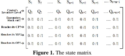
In the proposed DP, steps are time periods that are shown by n1, n2, .... In each step, some states are defined

and shown by Si. In the suggested method, we use

5(m+n+1) state matrix for each step, that n shows the number of Gs and m is the number of Rs. This matrix and its members are shown in Figure 1. Any decision changes the current state to next one. Two decisions are available in each step:

a) No tour between centers. Costs include holding of returns at Gs, Rs and CC, stock-out for Rs and penalty for landfill by Gs (if inventory exceeds MP).

b) Select a route and transfer returns between centers. Differnt routes can be selected, and each one impacts the next iteration decisions and costs. For this decision, ACO with the following characteristics is used in the model.

Each decision is shown by a matix D=[d1 d2 ... dn+m+2],

that implies how a state matrix changes to another. di

shows the inventory change at center i, that pick up is negative and deliver is positive. Other symbols are:

i

r Production / consumption amount at center i

i

d Pick-up (-)/deliver (+) returns at center i

i

MP Must Pick point for center i

i

CP Can Pick point for center i

i

OP Order Point for center i

i

LL The truck load before center i

i

L Pick up/deliver amount at center i

ij

d Distance between centers i and j

,.) (r

Si Row r of the new state (after decision D)

A transition function will change the current state (S) to next state (S') by decision D, that is shown as S'=F(S,D). The function for the first row of state matrix is as (25). Other rows will be calculated by this row amount.

i i i

i S d r

S(1,.) (1,.)  (25)

The objective function (total cost) for state S and decision D is shown by Z(S,D) and will be calculated by forward generation. For each iteration, objective function is calculated as the total costs of current iteration and reaching this iteration. As stated before, the tour selection for second decision (b) is taken by a hybrid algorithm of ACO and TS, with the following steps.

Step 1. Ants population is the number of trucks at CC at the first iteration. They must select the best route for picking up and delivering returns.

α and β are coefficients for the importance of landfill penalty for Gs (pickup when reach MP) and stock-out for the Rs, respectively These coefficients that are calculated by costs (28), give priorities to the more important routes.

ij i i

j j ij

d L LL TP

y x T

 

  

  .

) 0

( ₍₂₆₎

ij i i

j j ij

d L LL

O S T

 

 

  .

) 0

( (27)

U L

S

U L

P

C C

C C

C C

  

 

 , (28)

Step 2. The pheromone amount between two centers at time t+1 is calculated by Equation (29), that 1-ρ stands for evaporation rate and the amount of pheromones made by kth ant between centers i and j is k

ij t

 .

(29)

k ij ij

ij t T t T

T ( 1) ()

k ij T

 _{calculation is different in different ACO algorithms.}

We used Equation (30) when truck goes from I to j, that is derived from ant number method and Q is constant.

ij i i k

ij

d L LL

Q t

t T

    

 (, 1) ₍₃₀₎

TS concepts are used to help ants in finding a good route. This technique's performance at VRP has been evidenced in prior literature [27]. Tabu list is a set of rules to ban some solutions from appearing in the answers. According to their memory structure, the tabu lists are categorized into short, intermediate and long-terms [28]. Tabui is the tabu list for current iteration.

Long term and short term tabu lists are used here. In long-term tabu list, the centers that vehicle passed before this iteration and at this iteration are listed and must not be selected any more until the tour finishes. Short-term tabu includes the centers that truck can not go from the current center and lasts only one iteration. For example, if a truck does not have remaining capacity, all Gs are at short-term list. If truck delivers a part of its returns, at the next iteration some Gs can be removed from this list. A truck starts its tour at CC and can pick up some returns. If sum of amounts that must be picked from Gs is more than sum of deliveries at Rs, the amount of loads to pick up at CC will be zero. Otherwise, it is calculated by Equation (31).





_



_

 CC i i

CC I TP U L

L min , , (31)

Step 3. When a truck moves into another center, its load will be updated and the next center (j) will be determined according to remained pheromone of each route based on Equation (32). b is a constant that stands for the importance ratio between distance and pheromone amount and considered 1 in our model.

    

 

      

otherwise number

max ₀

random

q q if Tabu u d T

j b i

iu iu

(32)

q is a random number between zero and one and q0 is a

constant that helps in finding a random route with distribution function shown in Equation (33).

    

 



_

otherwise 0

Tabu j )

( i

i

tabu u

b iu iu b ij ij

ij T d

d T

P (33)

Step 4. After each answer, the pheromone amount for routes are updated, short-term and long-term tabu lists are deleted and fitness function (total cost) is calculated.

Step 5. For the next ants (trucks), the remained pheromone at each route is considered as the initial pheromone amount and the previous steps are repeated. Each answer is shown as a two row matrix. The first row shows the number of centers that returns are picked up or delivered. CC is the first and last cell of this row, meaning that start and finish of a tour is at CC. The second row stands for the amount of pick up (-) or deliver (+) at each center. The general answer matrix and a sample answer are shown in Figure 2. This answer means that 50 units of returns are picked up at CC, then truck goes to center 1, picks up 200 units, goes to center 2 picks up 250 units and delivers 200 units at center 5 and 300 units at center 7 and comes back to CC.

Step 6. The minimum amount of fitness function is selected as fbest and its route as rbest.

Step 7. To increase the number of anwers and improve them, differnet permutations of the centers between start and finish are created. If fitness function of one answer is better than fbest, it replaces rbest. The second row of the answer matrix, the number of columns, minimum and maximum of each cell are shown by hi, nn, LLLi and ULLi, respectively. By these

symbols, the permutations with the following situations are acceptable:

j h

j

i i 



1 0

(34)

0

1 





n

i hi (35)

i i

i h ULL

LLL  (36)

Equation (34) shows that the sum of pick up at each point must be more than or qual to deliveries.

Figure 2. The answer matrix

Also the total amount of picked up returns are delivered to ceters (35). The upper and lower bound of xi are

shown in (36). For Gs, upper level is the inventory of center and lower level is CP. for Rs, upper level is EOQ and lower level is OP.

Step 8. The best route and fitness function are shown by rbest and fbest. By finding these values, the best solution (di) will be achieved. Answer (D) obtained

from ACO is used to calculate the next state by (25) and S', D and objective function. For each iteration, total cost is the result of summing this iteration fitness function and previous steps'. Finaly 2n costs are calculated (n: number of periods). Optimal route is the minimum cost.

6. NEUMERICAL EXAMPLE

Since the model is a MINLP with a lot of integer, binary and continuous variables, solving with commercial solvers to compare with our algorithm is not possible. Therefore, the solved problems in previous cases [16, 17, 19, 23, 29] are evaluated against the current algorithm. In searching for solved IRPs, it is shown that the type of usual IRPs are differnt from our problem. The literature cases usually took place in forward supply chains and contained one producer and some customers. But in current problem there is another type of center (CC), that is not producer and not customer. Some other differences are at Table 2. The distinctions also show the model innovation beside previous IRPs.

With the differences, in order to compare the current solution by previous ones, we have to change some assumptions and relax the model. Therefore, CC is deleted, just one G is considered as a producer since it makes returns. By these assumptions, the algorithm is coded and solved via Matlab 2013.

TABLE 2. Characteristics of studied problems

Characteristic Previous cases Current problem

Centers' kind Producer, customer Producer, customer, collection center Number of Producers Single Multiple Start and finish of each

tour One point (producer) One point (CC) Inventory policy OU2_/ML3 _EOQ Pick up time at Gs No matter CP and MP points Deliver time at Rs No matter Order point

2_{Order-Up-To Level} 3_{Maximum Level}

Also Rs are considered as customers. Production and consumption rates, initial inventory levels, distance between centers, holding and transportation costs are known in the solved examples. Furthermore, to validate our model by the inventory policies of literature, EOQ is considered as maximum inventory, production rate as OP and truck capacity as MP point.

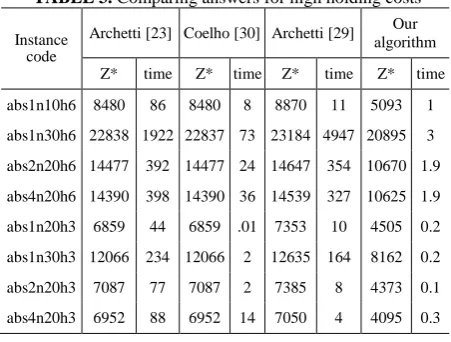
The instances of Archetti et al. are driven from coelho site4, solved for at least 50 times and the time and objective functions are calculated. Table 3 shows some of the comparisons between instances for high holding costs, solved by the proposed algorithm and three previous researches. The first column reports the instance code, as suggested by Archetti et al. [23]. The tables show about 35% decrease in the average objective function (total cost) and 100% decrease in average solving time. The objective function in these three references contains holding cost at different centers and transportation between them. In some works [23] it contains also penalty for infeasibility of routes, and Coelho's [30] objective function added transshipment cost. Our objective function also consists of the first two costs plus penalty for not covering Gs, stock out, loading, unloading and starts costs. To be comparable, the loading, unloading and start costs are omitted.

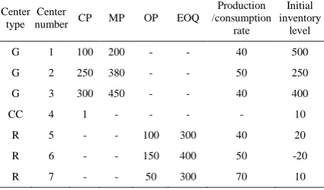
Despite the differences between solved instances and our problem in reverse supply chain, the high decrease in time and objective function prove the algorithm's capability to solve similar problems. To solve our problem in reverse supply chain, we consider a small problem by three return generators (G), three recovery centers (R) and one CC as described in Table 4.

The problem is solved for about 300 times and the results show that permutation decreases objective function just about 0.04%, but increase the solution time about 240%.

TABLE 3. Comparing answers for high holding costs

Instance code

Archetti [23] Coelho [30] Archetti [29] Our algorithm

Z* time Z* time Z* time Z* time

abs1n10h6 8480 86 8480 8 8870 11 5093 1

abs1n30h6 22838 1922 22837 73 23184 4947 20895 3

abs2n20h6 14477 392 14477 24 14647 354 10670 1.9

abs4n20h6 14390 398 14390 36 14539 327 10625 1.9

abs1n20h3 6859 44 6859 .01 7353 10 4505 0.2

abs1n30h3 12066 234 12066 2 12635 164 8162 0.2

abs2n20h3 7087 77 7087 2 7385 8 4373 0.1

abs4n20h3 6952 88 6952 14 7050 4 4095 0.3

TABLE 4. Characteristics of centers in our problem

By this result, removing permutation from algorithm, may optimize the algorithm's performance.

In order to define the optimum parameters of ACO in our algorithm, design of experiments is used. Four factors: number of initial solutions, evaporation rate, Q in the formula of pheromonesamount (step 2) and q0 in

the formula of next point (step 3) and three levels for each are assumed. Then about 10 combination of these facors are made, each model run for twenty times and average total cost and solution time is calculated. Results of the analysis by minitab 13 illustrate that the best combination of parameters for ACO is as:

ant number =10 ρ = 0.5 Q = 10 q0 = 0.9

To describe the robustness of our algorithm, Equation (37) is used as suggested by [12].

(37)



O O O O



Robustness  , 

In this formulation O is the average and O is the

variance of objective function in different runs. A smaller range illustrates more robustness of the algorithm. Results of different trial combinations demonstrate that the selected one is the third according to its robustness and is equal to (52122530, 52124546).

7. ANALYSIS AND DISCUSSION

Inventory-Routing Problems are of the important probelms, especially by gaining acceptance of VMI in supply chains. However, these type of problems are seldom studied in reverse supply chains. Since the members and relationships between them are different in reverse supply chains, the probems and solving differ in these chains. In the current paper, firstly a method to collaborate beween different members of reverse supply chains is developed and modeled mathematically. Since the IRP model is categorized as NP-hard, a hybrid huristic model is proposed to solve the model by a combination of DP, ACO and TS. To evaluate the model, firstly instances from earlier papers are solved and their time ad cost are determined. After assuring the performance of model by decreasing costs, the model is

used for a small problem in a reverse supply chain and the best combination of factors for ACO part of algorithm is identified.

The results suggest that IRP in reverse supply chains could be extended to consider other variations of collaboration by future researhers. For example by new inventory policies for different members, removing CC, adding more CCs and for multiple products and recovery policies. Since uncertainty is a characteristic of reverse supply chains, considering it in future studies can be a wide research area.

8. REFERENCES

1. Zhang, Y. and Sun, J., "Cooperation in reverse logistics", in ICEB., (2004), 63-67.

2. Le Blanc, H.M., "Closing loops in supply chain management: Designing reverse supply chains for end-of-life vehicles.", Tilburg University, School of Economics and Management, (2006).

3. Alaei, S. and Setak, M., "Designing of supply chain coordination mechanism with leadership considering".

4. Poirier, C., Swink, M. and Quinn, F., "The fifth annual global survey of supply chain progress", Computer Science Corporation, (2007).

5. Hudnurkar, M., Jakhar, S. and Rathod, U., "Factors affecting collaboration in supply chain: A literature review", Procedia-Social and Behavioral Sciences, Vol. 133, (2014), 189-202. 6. Hernandez, J.E., Poler, R., Mula, J. and Lario, F.C., "The reverse

logistic process of an automobile supply chain network supported by a collaborative decision-making model", Group Decision and Negotiation, Vol. 20, No. 1, (2011), 79-114. 7. Vallet-Bellmunt, T., Martinez-Fernandez, M.T. and

Capó-Vicedo, J., "Supply chain management: A multidisciplinary content analysis of vertical relations between companies, 1997– 2006", Industrial Marketing Management, Vol. 40, No. 8, (2011), 1347-1367.

8. SETAK, M. and Daneshfar, L., "An inventory model for deteriorating items using vendor-managed inventory policy",

International Journal of Engineering-Transactions A: Basics, Vol. 27, No. 7, (2014), 1081-1090.

9. Akhbari, M., Zare Mehrjerdi, Y., Khademi Zare, H. and Makui, A., "A novel continuous knn prediction algorithm to improve manufacturing policies in a vmi supply chain", International Journal of Engineering, Transactions B: Applications, Vol. 27, (2014), 1681-1690.

10. Pokharel, S. and Mutha, A., "Perspectives in reverse logistics: A review", Resources, Conservation and Recycling, Vol. 53, No. 4, (2009), 175-182.

11. Bai, H., "Reverse supply chain coordination and design for profitable returns-an example of ink cartridge", Worcester Polytechnic Institute, (2009),

12. Lambert, S., Riopel, D. and Abdul-Kader, W., "A reverse logistics decisions conceptual framework", Computers & Industrial Engineering, Vol. 61, No. 3, (2011), 561-581. 13. Aras, N., Aksen, D. and Tekin, M.T., "Selective multi-depot

vehicle routing problem with pricing", Transportation Research Part C: Emerging Technologies, Vol. 19, No. 5, (2011), 866-884.

14. Gou, Q., Liang, L., Xu, C. and Zhou, C., "A modification for a centralized inventory policy for an open-loop reverse supply chain: Simulation and comparison", in Proceedings of 2007 Center

type Center

number CP MP OP EOQ

Production /consumption

rate

Initial inventory

level

G 1 100 200 - - 40 500

G 2 250 380 - - 50 250

G 3 300 450 - - 40 400

CC 4 1 - - - - 10

R 5 - - 100 300 40 20

R 6 - - 150 400 50 -20

International Conference on Management Science and Engineering Management, Citeseer., (2007), 223-230.

15. Gou, Q., Liang, L., Huang, Z. and Xu, C., "A joint inventory model for an open-loop reverse supply chain", International Journal of Production Economics, Vol. 116, No. 1, (2008), 28-42.

16. Coelho, L.C., Cordeau, J.-F. and Laporte, G., "Thirty years of inventory routing", Transportation Science, Vol. 48, No. 1, (2013), 1-19.

17. Coelho, L.C., Cordeau, J.-F. and Laporte, G., "The inventory-routing problem with transshipment", Computers & Operations Research, Vol. 39, No. 11, (2012), 2537-2548.

18. Razavi, M.K. and Nik, E.R., "Meta heuristic for multi depot inventory routing problem backlogging", Journal of Basic and Applied Scientific Research, Vol. 3, No. 2s, (2013), 273-280. 19. Mirzaei, A.H., Nakhai, K.I. and Zegordi, S.H., "A new

algorithm for solving the inventory routing problem with direct shipment", (2011).

20. Mes, M., Schutten, M. and Rivera, A.P., "Inventory routing for dynamic waste collection", Waste Management, Vol. 34, No. 9, (2014), 1564-1576.

21. Srivastava, S.K., "Network design for reverse logistics", Omega, Vol. 36, No. 4, (2008), 535-548.

22. Rogers, D.S. and Tibben-Lembke, R.S., "Going backwards: Reverse logistics trends and practices, Reverse Logistics Executive Council Pittsburgh, PA, Vol. 2, (1999).

23. Archetti, C., Bertazzi, L., Hertz, A. and Speranza, M.G., "A hybrid heuristic for an inventory routing problem", Informs Journal on Computing, Vol. 24, No. 1, (2012), 101-116. 24. Steeman, Q., "The vehicle routing problem with drop yards: A

dynamic programming approach", (2012).

25. Pillac, V., Gendreau, M., Guéret, C. and Medaglia, A.L., "A review of dynamic vehicle routing problems", European Journal of Operational Research, Vol. 225, No. 1, (2013), 1-11.

26. Tan, W.F., Lee, L.S., Majid, Z.A. and Seow, H.V., "Ant colony optimization for capacitated vehicle routing problem", Journal of Computer Science, Vol. 8, No. 6, (2012), 846.

27. Fakhrzada, M. and Esfahanib, A.S., "Modeling the time windows vehicle routing problem in cross-docking strategy using two meta-heuristic algorithms", International Journal of Engineering-Transactions A: Basics, Vol. 27, No. 7, (2013), 1113.

28. Glover, F., "Tabu search: A tutorial", Interfaces, Vol. 20, No. 4, (1990), 74-94.

29. Archetti, C., Bertazzi, L., Laporte, G. and Speranza, M.G., "A branch-and-cut algorithm for a vendor-managed inventory-routing problem", Transportation Science, Vol. 41, No. 3, (2007), 382-391.

30. Coelho, L.C., "Flexibility and consistency in inventory-routing", PhD thesis, Montreal, Canada: University of Montreal, (2012).

A Hybrid Dynamic Programming for Inventory Routing Problem in Collaborative

Reverse Supply Chains

M. Moubeda_{, Y. Zare Mehrjerdi}b

a _{Department of Industrial Engineering, Faculty of Engineering, Ardakan University} b _{Department of Industrial Engineering, Faculty of Engineering, Yazd University}

P A P E R I N F O

Paper history: Received 21 April 2015

Received in revised form 09 August 2016 Accepted 25 August 2016

Keywords: Reverse Supply Chains Collaboration Dynamic Programming Ant Colony Optimization Tabu search

ديكچ ه

یثبیزیسه لئبسه

-( یدَجَه

IRP

يیا ىبهشوّ ىدَوً ٌِیْث یازث یدَجَه تیزیذه ٍ ِیلقً لیبسٍ یثبیزیسه سا یجیکزت ،)

ِکجض رد تکربطه یسبسلذه رَظٌه ِث ٍر صیپ ِلبقه رد .تسا لئبسه ُزیجًس سا یا

لدبؼه یضٍر سا ،سَکؼه يیهأت یبّ

َجَه تیزیذه ( ُذٌضٍزف طسَت ید

VMI

ُزیجًس رد ) يیا یضبیر یسبسلذه ِجیتً .تسا ُذض ُدبفتسا یتٌس يیهأت یبّ

ِلئسه ،تکربطه عًَ سا یا

IRP

ُزیجًس رد .تسا ُدَث ،یتطگسبث یلابک ُذٌٌکذیلَت يیذٌچ ،ِؼلبطه درَه سَکؼه يیهأت یبّ

یثبیسبث يیذٌچ غوج شکزه کی ٍ ُذٌٌک

شٍر سا ىآ لح ،لذه دبیس یگذیچیپ لیلد ِث .ذًراد دَجٍ بّلابک يیا یرٍآ یبّ

تقٍ ،ُذیچیپ لَوؼه سا یربکتثا شٍر کی اذل .تسا يکوهزیغ تبقٍا یخزث ٍ زیگ

ِهبًزث تیکزت نتیرَگلا ،بیَپ یشیر

لئبسه ،یدبٌْطیپ شٍر دزکلوػ سا ىبٌیوطا رَظٌه ِث .تسا ُذض دبٌْطیپ لذه لح یازث عٌَوه یَجتسج ٍ ىبگچرَه ُار يیا جیبتً ِسیبقه .ذض لح شیً نتیرَگلا يیا سا ُدبفتسا بث يیطیپ تبؼلبطه رد ُذض حزط ًَِوً لح

یه ىبطً بّ ِک ذّد

یدبٌْطیپ شٍر ِظحلاه لثبق زیثأت

ٌِیشّ صّبک زث یا فلتخه یبّزیغته راذقه يییؼت رَظٌه ِث .تسا ِتضاد لح ىبهس ٍ بّ

یبّزتهاربپ ٌِیْث راذقه ٍ ُذیدزگ ةبختًا ماذک زّ یازث حطس ِس ٍ لهبػ ربْچ ،تبطیبهسآ یحازط سا ُدبفتسا بث نتیرَگلا ا ُذض فیزؼت لئبسه ًَِگٌیا لح یازث ىبگچرَه نتیرَگلا .تس