Open Access
Research article
Rasch fit statistics and sample size considerations for polytomous
data
Adam B Smith*
1,2, Robert Rush
3, Lesley J Fallowfield
4, Galina Velikova
†1and
Michael Sharpe
†5Address: 1Cancer Research UK – Clinical Centre, St. James's University Hospital, Leeds, UK, 2Centre for Health & Social Care, University of Leeds, Leeds, UK, 3Centre for Integrated Health Research, Queen Margaret University, Edinburgh, UK, 4Psychosocial Oncology Group – Cancer Research UK, University of Sussex, UK and 5School of Molecular & Clinical Medicine, University of Edinburgh, Edinburgh, UK
Email: Adam B Smith* - [email protected]; Robert Rush - [email protected]; Lesley J Fallowfield - [email protected]; Galina Velikova - [email protected]; Michael Sharpe - [email protected]
* Corresponding author †Equal contributors
Abstract
Background: Previous research on educational data has demonstrated that Rasch fit statistics (mean squares and t-statistics) are highly susceptible to sample size variation for dichotomously scored rating data, although little is known about this relationship for polytomous data. These statistics help inform researchers about how well items fit to a unidimensional latent trait, and are an important adjunct to modern psychometrics. Given the increasing use of Rasch models in health research the purpose of this study was therefore to explore the relationship between fit statistics and sample size for polytomous data.
Methods: Data were collated from a heterogeneous sample of cancer patients (n = 4072) who had completed both the Patient Health Questionnaire – 9 and the Hospital Anxiety and Depression Scale. Ten samples were drawn with replacement for each of eight sample sizes (n = 25 to n = 3200). The Rating and Partial Credit Models were applied and the mean square and t-fit statistics (infit/outfit) derived for each model.
Results: The results demonstrated that t-statistics were highly sensitive to sample size, whereas mean square statistics remained relatively stable for polytomous data.
Conclusion: It was concluded that mean square statistics were relatively independent of sample size for polytomous data and that misfit to the model could be identified using published recommended ranges.
Background
Although Rasch Models [1] were originally designed and used for educational assessment in recent years they have increasingly been used in health research. This renewed interest in these models has largely been encouraged by a number of potential advantages of Rasch models over
tra-ditional psychometric methods, including the ability to decrease the number of items in questionnaires to reduce patient burden whilst retaining the psychometric proper-ties of the instrument, and the pooling of data drawn from different samples allowing more accurate parameter esti-mation. Recent studies in health have explored the use of
Published: 29 May 2008
BMC Medical Research Methodology 2008, 8:33 doi:10.1186/1471-2288-8-33
Received: 22 January 2008 Accepted: 29 May 2008
This article is available from: http://www.biomedcentral.com/1471-2288/8/33
© 2008 Smith et al; licensee BioMed Central Ltd.
Rasch models in instrument development [2-4], modifi-cation of existing questionnaires [5-8], as well as in instru-ment and cross-linguistic comparison [9,10].
Rasch Models are a family of measurement models [11] which can be used to describe latent traits where items from questionnaires and person scores are located along the same scale of the latent trait. Item location ("difficul-ties") and person measures ("abili("difficul-ties") are estimated sep-arately to produce estimates for each parameter which are sample and item independent respectively [12]. Rasch Models specify a number of criteria, which if fulfilled result in interval scales where adjacent scores along the scale are equally spaced, a feature which is particularly important for interpreting clinically meaningful differ-ences [13]. Firstly, the data should describe a unidimen-sional construct, that is, a single latent trait should explain the variance in the data. The existence of dimensionality can be assessed using principal components analyses of the residuals [14]. Secondly, item invariance stipulates that item (or person) parameters should be independent of the sample (or items) used. This item invariance crite-rion can be evaluated using differential item functioning to determine whether item bias is present. The final crite-rion, which will form the focus of this paper, is item fit, in other words whether individual items in a scale fit the Rasch model.
There has been and there continues to be a considerable debate around the issue of which is the most appropriate fit statistic to use, what range of fit statistics to be employed when evaluating fit, and how fit statistics should be interpreted [15,16].
The use of chi-square statistics or infit and outfit mean squares to assess item fit to the model (described in more detail below) has been advocated. The mean squares can be converted through a cube-root transformation (Wil-son-Hilferty) to (infit/outfit) t-statistics.
The mean square fit statistics are perhaps the most com-monly used fit statistics in health research. A series of ranges has been suggested [17] to be employed when eval-uating item fit depending on the type of test, however the majority of studies employ a range of 0.7 to 1.3. Despite the popularity of this approach some concerns have been voiced about the use of a single, universal range to evalu-ate fit and the lack of adjustment of the range to sample size. For instance, Smith et al. [16] using simulated data-sets on dichotomous data have determined that Type I error rates (defined here as the probability of falsely reject-ing an item as not fittreject-ing the Rasch model) were signifi-cantly less than α = 0.05 for both infit and outfit mean squares using a range of critical values (0.7, 0.8, 0.9 – 1.1, 1.2, 1.3). Furthermore, Type I error rates decreased for the
outfit mean square as sample size was increased. In con-trast, the Type I error rates for the t-statistics, although not equal to 5% demonstrated fewer discrepancies.
More recently, studies [18] have demonstrated using data collected from a large sample of examinees' results that t-statistics may potentially identify more items that do not fit the model than both the infit and outfit mean square fit statistics. For instance, the number of misfitting items identified by the t-statistic was four times greater than those identified by the mean square fit statistic (23 and 5, respectively).
In addition to research on the dichotomous model, recent work on the polytomous (Rating Scale) model with simu-lated data has suggested that the variability of mean squares is dependent on sample size and furthermore that the standard deviations for the t-statistics are generally smaller than their expected value (unity) [19]. These authors propose adjusting the critical range employed for both types of fit statistic depending on sample size.
Finally, Smith & Suh [18] have concluded that using mean square statistics may lead researchers to missing signifi-cant numbers of misfitting items, which may have an important impact on the development of unidimensional instruments, and that there is, furthermore, a need to understand Type I error rates associated with critical val-ues for fit statistics. On the basis of this Smith and col-leagues [16,18] have suggested that the t-statistic rather than the weighted and unweighted mean squares should be used to identify misfit, given that this statistic appears to be less sensitive to changes in sample size or alterna-tively to adjust mean square fit statistics using a correction based on the square root of the sample size [16].
However, despite this assertion there are a number of other methodological studies [15,20] which have shown that the t-statistic is highly sample dependent.
Therefore the aim of this study was to investigate the impact of sample size on four commonly used fit statis-tics, i.e. infit/outfit mean square and their t-statistics for two polytomous Rasch models using data collected from a cancer patient sample.
The study attempted to determine: 1). whether fit statistics (and therefore Type I error rates, i.e. the probability of falsely rejecting an item which does fit the Rasch model) vary with sample size and 2). whether there were any dif-ferences in this variation between the different types of fit statistic.
Methods
Participants
Patient data were pooled from a number of studies carried out by Cancer Research – UK Psychological Medicine Group, Western General Hospital, Edinburgh (Scotland) over the past decade. The data have been collated from patients who completed a touchscreen version of both the HADS and the PHQ-9 in outpatient oncology clinics.
A total of 4072 patients completed the HADS (2781 females and 1291 males), and 3556 patients completed the PHQ-9 (2268 females and 1288 males). The average age of the sample was 60 years. Further clinical and demo-graphic details are available from the published studies [21].
The studies from which these data have been drawn have all received ethical approval from the local research ethics committee.
Instruments
The Hospital Anxiety & Depression Scale (HADS)
The Hospital Anxiety and Depression Scale (HADS) [22] was originally developed for screening for psychological distress in the general medical population. The scale con-sists of 7 items forming a Depression subscale (HADS-D), and 7 items forming an Anxiety subscale (HADS-A). Patients are asked to rate how they have felt in the past week on a 4-point scale (scored 0–3). It has been claimed that scores on the two subscales may also be summed to provide a total score (HADS-T), measuring psychological distress [23]. Previous research in a large heterogeneous cancer population [6] has shown potential misfit on three of the instruments' items: Anxiety 6 ("I get a sort of fright-ened feeling") and Depression 5 and 7 ("I have lost inter-est in my appearance" and "I can enjoy a good book, radio or TV programme" respectively). This misfit was present both in the full, 14-item version of the HADS as well as for the individual subscales. Although a principal compo-nents analysis of the residuals did not reveal the presence of any additional factors, given the misfitting items the
analysis presented here will focus on the two subscales, HADS-Anxiety (A) and HADS-Depression (D).
Patient Health Questionnaire (PHQ-9)
The Patient Health Questionnaire – 9 (PHQ-9) [24] is a nine-item self-administered questionnaire which may be used for detecting and assessing the severity of depression. The instrument is based on the Diagnostic and Statistical Manual of Mental Disorders (DSM-IV) [25] criteria for diagnosing depression, and is scored on a 4-point scale ("not at all" to "nearly every day"). Patients are asked to rate any problems experienced over the last two weeks.
Rasch Models
Both the Rating Scale and Partial Credit models are mem-bers of the family of Rasch Models [1]. The Rating Scale Model [26] is commonly employed to analyse Likert-type data [see Additional file 1]. As with all Rasch Models, the Rating Scale describes a probabilistic relationship between item difficulty (D) and person ability (B). In addition to this, thresholds are derived for each adjacent response category in a scale. In general, for k response cat-egories, there are k-1 thresholds. Each threshold has its own estimate of difficulty (Fk). The Rating Scale Model [see Additional file 1] describes the probability, Pni of a person with ability Bn, choosing a given category with a threshold Fk and item difficulty Di. A single set of thresh-olds is estimated for all items in a scale. The Partial Credit Model [27] can be seen as a modification of the Rating Scale Model where the threshold estimates are not con-strained, that is, threshold estimates are free to vary between each item within a scale. Therefore for N items there will be N(k – 1) threshold estimates for the Partial Credit Model.
Rasch Fit Statistics
Rasch fit statistics describe the fit of the items to the model. The mean square fit statistics have a chi-square dis-tribution and an expected value of 1, where fit statistics greater than 1 can be interpreted as demonstrating more variation between the model and the observed scores, e.g. a fit statistic of 1.25 for an item would indicate 25% more variation (or "noise") than predicted by the Rasch model [11], in other words there is an underfit with the model. Conversely, an item with a fit statistic of 0.70 would indi-cate 30% less variation (or "overlap") than predicted or the items overfit the model. Items demonstrating more variation than predicted by the model can be considered as not conforming to the unidimensionality requirement of the Rasch model.
standardised residuals for each item/person interaction [see Additional file 1]. The outfit mean square is the aver-age of the standardised residual variance across items and persons and is unweighted, meaning that the estimate produced is relatively more affected by unexpected responses distant to item or person measures. For the infit mean square the residuals are weighted by their individ-ual variance (Wni) [see Additional file 1] to minimise the impact of unexpected responses far from the measure. The infit mean square is relatively more affected by unex-pected responses closer to item and person measures [11].
The infit and outfit mean squares can be converted to an approximately normalised t-statistic using the Wilson-Hilferty transformation [see Additional file 1]. These infit/ outfit t-statistics have an expected value of 0 and a stand-ard deviation of 1. These statistics are evaluated against ± 2, where values greater than +2 are interpreted as demon-strating more variation than predicted.
Method
The relationship between sample size and fit statistics was explored using the two Rasch models, that is, the Rating Scale Model [26], and Partial Credit Model [27]. The anal-ysis was performed using Winsteps version 3.64 [14]. Eight sample sizes were used for each questionnaire: 25, 50, 100, 200, 400, 800, 1600, and 3200. Ten samples were drawn with replacement for each sample size for each item for the two instruments. Therefore, for the HADS
there were 1120 data points (14 items × 8 sample sizes × 10 samples), and 720 data points for the PHQ-9 (9 items × 8 samples sizes × 10 samples). Ten samples were col-lated for each sample size (25 to 3600) for each question-naire to produce an average for each of the four fit statistics (infit/outfit mean squares (MNSQ) and t-statistic (ZSTD in Winsteps)) for each item. This process was com-pleted for both Rasch models.
Results
1. Fit Statistics – Type I error rate
Tables 1, 2, 3, 4 show the fit statistics for each item aver-aged across sample size and provide an indication of the Type I error rates. For both the HADS subscales and PHQ-9 a Type I error rate of 5% would translate into approxi-mately 1 misfitting item identified by chance alone.
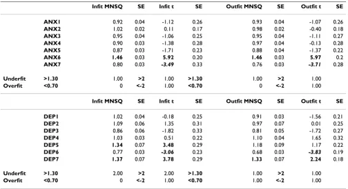
Tables 1 and 2 demonstrate that for both HADS subscales there was a broad agreement between the infit and outfit statistics. In other words, the numbers of items identified as misfitting were relatively consistent for the infit and outfit versions of the same type of statistic irrespective of the Rasch model applied.
However for the PHQ-9 (Tables 3 and 4) consistently more items were identified as misfitting by t-statistics (infit/outfit t-statistic) than by the equivalent mean square statistics. In terms of underfit to the model the Type I error rate for the t-statistics was at least double that
Table 1: Fit statistics for the HADS subscale items (collapsed across sample size) for the Rating Scale Model
Infit MNSQ SE Infit t SE Outfit MNSQ SE Outfit t SE
ANX1 0.92 0.04 -1.12 0.26 0.93 0.04 -1.07 0.26
ANX2 1.02 0.02 0.11 0.17 0.98 0.02 -0.40 0.18
ANX3 0.95 0.04 -1.06 0.25 0.95 0.04 -1.11 0.27
ANX4 0.90 0.03 -1.38 0.28 0.97 0.04 -0.13 0.28
ANX5 0.87 0.03 -1.71 0.23 0.88 0.04 -1.37 0.22
ANX6 1.46 0.03 5.92 0.20 1.46 0.03 5.97 0.2
ANX7 0.80 0.03 -3.49 0.33 0.76 0.03 -3.71 0.28
Underfit >1.30 1.00 >2 1.00 >1.30 1.00 >2 1.00
Overfit <0.70 0 <-2 1.00 <0.70 0 <-2 1.00
Infit MNSQ SE Infit t SE Outfit MNSQ SE Outfit t SE
DEP1 1.02 0.04 -0.18 0.25 0.91 0.03 -1.56 0.21
DEP2 1.09 0.06 1.35 0.31 0.97 0.07 0.01 0.25
DEP3 0.86 0.06 -1.82 0.33 0.81 0.05 -1.72 0.27
DEP4 1.03 0.03 0.51 0.22 1.10 0.04 1.65 0.32
DEP5 1.34 0.07 3.48 0.29 1.18 0.09 1.17 0.22
DEP6 0.77 0.03 -3.06 0.23 0.68 0.03 -3.83 0.19
DEP7 1.37 0.07 3.78 0.29 1.33 0.07 2.24 0.18
Underfit >1.30 2.00 >2 2.00 >1.30 1.00 >2 1.00
of the corresponding mean square, e.g. for the Rating Scale Model, the total number of items exceeding the thresholds for infit t-statistic was 3, whereas for the infit mean square 1, and for the Partial Credit Model infit t-sta-tistic it was 2, and the infit mean square 0. A similar pat-tern of results was also found for those items overfitting the models.
Finally, it can also be seen that the standard errors were uniformly smaller for the mean square statistics than those for the t-statistics, indicating greater levels of stabil-ity in the parameter estimates. This was particularly
noticeable for the HADS, but also applied to some extent to the PHQ-9.
2. Fit Statistics – Sample Size
The relationship between sample size and fit statistics is shown in Tables 5, 6, 7, 8. This analysis has been broken down into overfitting (MNSQ < 0.7/t < -2) and underfit-ting/misfitting items (MNSQ > 1.3/t > 2).
Overfitting items
It can be seen that for both the infit and outfit mean squares few items were identified with mean square fit sta-tistics < 0.7 for the HADS subscales (Tables 5 and 7) and
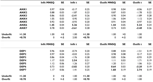
Table 2: Fit statistics for the HADS subscale items (collapsed across sample size) for the Partial Credit Model
Infit MNSQ SE Infit t SE Outfit MNSQ SE Outfit t SE
ANX1 0.97 0.04 -0.17 0.25 0.98 0.04 -0.06 0.27
ANX2 0.88 0.03 -1.87 0.23 0.87 0.03 -1.78 0.22
ANX3 0.86 0.03 -2.41 0.26 0.90 0.04 -1.89 0.28
ANX4 1.05 0.03 0.95 0.23 1.06 0.04 1.12 0.24
ANX5 0.92 0.03 -0.93 0.20 0.91 0.04 -0.97 0.22
ANX6 1.45 0.04 5.36 0.22 1.44 0.05 5.24 0.24
ANX7 0.78 0.03 -3.61 0.28 0.74 0.03 -3.48 0.26
Underfit >1.30 1.00 >2 1.00 >1.30 1.00 >2 1.00
Overfit <0.70 0 <-2 2.00 <0.70 0 <-2 1.00
Infit MNSQ SE Infit t SE Outfit MNSQ SE Outfit t SE
DEP1 0.96 0.04 -0.74 0.20 0.88 0.04 -1.51 0.19
DEP2 0.97 0.04 -0.03 0.25 0.98 0.08 0.17 0.23
DEP3 0.86 0.04 -1.76 0.28 0.85 0.06 -0.93 0.29
DEP4 1.17 0.03 2.54 0.21 1.11 0.03 1.71 0.19
DEP5 1.12 0.06 1.26 0.27 1.20 0.11 1.06 0.21
DEP6 0.73 0.03 -3.82 0.20 0.64 0.03 -3.20 0.19
DEP7 1.17 0.06 1.41 0.25 1.68 0.19 2.74 0.19
Underfit >1.30 0 >2 1.00 >1.30 1.00 >2 1.00
Overfit <0.70 0 <-2 1.00 <0.70 1.00 <-2 1.00
Table 3: Fit statistics for PHQ-9 items (collapsed across sample size) for the Rating Scale Model
Infit MNSQ SE Infit t SE Outfit MNSQ SE Outfit t SE
PHQ1 1.01 0.01 0.33 0.09 1.02 0.02 0.30 0.13
PHQ2 0.72 0.01 -4.04 0.08 0.71 0.01 -3.36 0.07
PHQ3 1.14 0.01 2.39 0.09 1.15 0.02 2.25 0.11
PHQ4 0.87 0.01 -2.09 0.09 0.93 0.01 -0.82 0.09
PHQ5 1.37 0.01 4.19 0.08 1.28 0.02 2.46 0.08
PHQ6 1.10 0.01 1.27 0.08 0.95 0.02 -0.42 0.07
PHQ7 1.04 0.01 0.60 0.08 0.86 0.01 -1.16 0.06
PHQ8 1.25 0.02 2.46 0.08 0.97 0.02 -0.08 0.07
PHQ9 1.17 0.03 1.48 0.10 0.84 0.05 -0.87 0.08
Underfit >1.30 1.00 >2 3.00 >1.30 0 >2 2.00
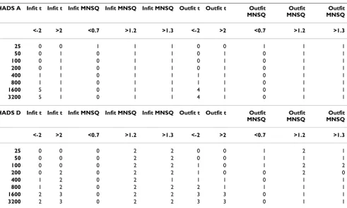
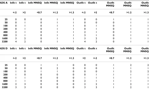
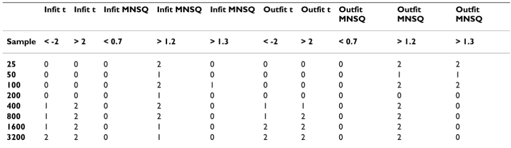
the PHQ-9 (Tables 6 and 8). In contrast to this, the corre-sponding t-statistics (< -2) demonstrated that as sample size increased, the number of items identified as misfit-ting rapidly increased. For instance, for the Ramisfit-ting Scale Model, the infit mean squares for HADS-D (Table 5) con-sistently failed to identify a single instance of an item mis-fitting as sample size increased, whereas the corresponding t-statistic identified no misfit between sample sizes 25 and 200. Furthermore, there was only 1 instance of misfit at sample sizes of 400 and 800, and 2
instances at sample sizes of 1600 and beyond. This pat-tern was particularly evident for the HADS-A Partial Credit Model (Table 7). A similar pattern was also observed for the PHQ-9 (Table 8).
Underfitting items
There was a clear link observed between sample size and fit statistic when comparing infit and outfit mean squares above 1.2 with t-statistics > +2. Once again, t-statistics increased in proportion to sample size, whereas the mean
Table 5: HADS – Rating Scale Model Error rates by sample size (collapsing across items)
HADS A Infit t Infit t Infit MNSQ Infit MNSQ Infit MNSQ Outfit t Outfit t Outfit MNSQ
Outfit MNSQ
Outfit MNSQ
<-2 >2 <0.7 >1.2 >1.3 <-2 >2 <0.7 >1.2 >1.3
25 0 0 1 1 1 0 0 1 1 1
50 0 1 0 1 1 0 1 0 1 1
100 0 1 0 1 1 0 1 0 1 1
200 0 1 0 1 1 0 1 0 1 1
400 1 1 0 1 1 1 1 0 1 1
800 1 1 0 1 1 1 1 0 1 1
1600 5 1 0 1 1 4 1 0 1 1
3200 5 1 0 1 1 4 1 0 1 1
HADS D Infit t Infit t Infit MNSQ Infit MNSQ Infit MNSQ Outfit t Outfit t Outfit MNSQ
Outfit MNSQ
Outfit MNSQ
<-2 >2 <0.7 >1.2 >1.3 <-2 >2 <0.7 >1.2 >1.3
25 0 0 0 2 2 0 0 1 2 1
50 0 0 0 2 2 0 0 1 1 1
100 0 0 0 2 2 1 0 1 2 2
200 0 2 0 2 2 1 0 0 2 0
400 1 2 0 2 1 1 1 0 1 1
800 1 2 0 2 2 2 1 1 1 1
1600 2 3 0 2 2 3 3 0 1 1
3200 2 3 0 2 2 3 3 0 1 1
The number of items exceeding the fit criteria are shown in each column
Table 4: Fit statistics for PHQ-9 items (collapsed across sample size) for the Partial Credit Model
Infit MNSQ SE Infit t SE Outfit MNSQ SE Outfit t SE
PHQ1 0.98 0.01 -0.02 0.09 0.96 0.02 -0.27 0.11
PHQ2 0.79 0.01 -2.99 0.07 0.74 0.01 -3.19 0.07
PHQ3 1.17 0.01 2.95 0.08 1.17 0.02 2.55 0.10
PHQ4 1.01 0.01 0.05 0.08 0.98 0.01 -0.25 0.08
PHQ5 1.22 0.01 2.47 0.08 1.30 0.03 1.93 0.09
PHQ6 0.95 0.01 -0.36 0.07 0.97 0.03 -0.26 0.08
PHQ7 0.91 0.01 -1.00 0.07 0.86 0.02 -1.04 0.07
PHQ8 1.05 0.02 0.34 0.08 0.95 0.03 -0.08 0.08
PHQ9 0.92 0.02 -0.22 0.06 1.00 0.10 -0.41 0.10
>1.30 0 >2 2.00 >1.30 0 >2 1.00
square equivalents remained approximately invariant to sample size changes (compare for instance the infit statis-tics on the Rating Scale for HADS-D in Table 5, as well as for the PHQ-9 in Table 6). Additionally, more instances of misfit were identified, in general, when a mean square of >1.2 was used compared with 1.3, although this was not always consistently the case.
3. Fit Statistics, Sample size and individual items
Items not demonstrating misfit
In terms of agreement between the four statistics for indi-vidual items not exhibiting misfit it can be seen from Table 1 that, for instance for HADS-A, the infit and outfit means squares agreed with their equivalent t-statistic on 5 items for the Rating Scale Model; similarly there was
agreement between the fit statistics for 4 items from the HADS-D. Slightly less consistency was observed for both subscales on the Partial Credit Model (Table 2) and for both models using the PHQ-9, although again there was agreement for the majority of items (Tables 3 and 4).
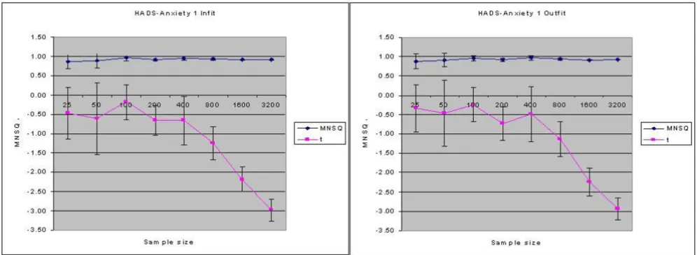
An example of an item (HADS-A1) which had demon-strated fit across all four statistics is shown in Figure 1. Although Table 1 demonstrated fit for the t-statistics it can be seen that whereas the item demonstrated consistent (infit and outfit) mean square statistics (approx. 0.92) across sample size, the infit and outfit t-statistics became increasingly more negative as sample size increased (> 200), resulting in the t-statistics highlighting significant overfit for this item at sample sizes greater than 1600.
Infit and Outfit statistics by sample size for HADS-Depression 6 Figure 2
Infit and Outfit statistics by sample size for HADS-Depression 6. Infit and Outfit statistics by sample size for HADS-Anxiety 1
Figure 1
Overfitting items
For the Rating Scale Model one HADS-A item (7) and one HADS-D item (6), as well as two PHQ-9 items (2 and 4) were identified as overfitting by the t-statistics but not by the mean squares. The Partial Credit Model demonstrated overfit for HADS-D6, as well as HADS-A3, and PHQ2. Fig-ure 2 demonstrates once again that whereas the mean squares remained consistent across sample size, the t-sta-tistics became increasingly more negative (sample size > 200).
Underfitting items
HADS-D5 and HADS-D7 were identified as underfitting on the Rating Scale Model (RSM) for both the in- and out-fit t-statistics, but not the mean squares, although neither was identified as misfitting on the Partial Credit Model (PCM); HADS-D4 was identified as misfitting (i.e. under-fitting) on the Partial Credit Model by the infit t alone. PHQ3 and 5 were identified as misfitting by both infit and outfit t-statistics for the RSM and PCM, but not by the mean squares. Finally, HADS-A item 6 was consistently identified as misfitting (underfitting) by all four statistics, yet when the four statistics are plotted against sample size
Table 7: HADS – Partial Credit Scale Model Error rates by sample size (collapsing across items)
HADS A Infit t Infit t Infit MNSQ Infit MNSQ Infit MNSQ Outfit t Outfit t Outfit MNSQ
Outfit MNSQ
Outfit MNSQ
<-2 >2 <0.7 >1.2 >1.3 <-2 >2 <0.7 >1.2 >1.3
25 0 0 0 1 1 0 0 1 1 1
50 0 1 0 1 1 0 0 0 1 1
100 0 1 0 1 1 0 1 0 1 1
200 0 1 0 1 1 0 1 0 1 1
400 2 1 0 1 1 2 1 0 1 1
800 3 1 0 1 1 3 1 0 1 1
1600 3 2 0 1 1 3 2 0 1 1
3200 4 2 0 1 1 4 2 0 1 1
HADS D Infit t Infit t Infit MNSQ Infit MNSQ Infit MNSQ Outfit t Outfit t Outfit MNSQ
Outfit MNSQ
Outfit MNSQ
<-2 >2 <0.7 >1.2 >1.3 >2 <-2 <0.7 >1.2 >1.3
25 0 0 1 1 0 0 0 1 2 2
50 0 0 0 2 0 0 0 1 1 1
100 1 0 1 1 0 0 0 1 2 2
200 1 0 0 0 0 0 1 1 1 1
400 1 1 0 0 0 1 1 1 1 1
800 1 1 0 0 0 2 1 1 1 1
1600 2 3 0 0 0 2 2 1 2 1
3200 3 3 0 0 0 3 3 1 2 1
Table 6: PHQ9 – Rating Scale Model Error rates by sample size (collapsing across items)
Infit t Infit t Infit MNSQ Infit MNSQ Infit MNSQ Outfit t Outfit t Outfit MNSQ
Outfit MNSQ
Outfit MNSQ
Sample < -2 > 2 < 0.7 > 1.2 > 1.3 < -2 > 2 < 0.7 > 1.2 > 1.3
25 0 0 0 0 2 0 0 0 0 2
50 0 0 0 1 0 0 0 0 0 1
100 0 1 1 0 1 0 0 1 0 1
200 1 1 0 0 2 1 0 0 0 0
400 1 3 0 0 1 1 1 0 0 0
800 2 3 1 0 1 1 2 2 0 0
1600 2 5 0 0 1 2 2 0 0 0
(Figure 3) it is apparent that this item was only identified by the t-statistics as under/misfitting once the sample size exceeded 200.
In summary, two instances of misfit for the t-statistics could be discerned from the data: 1). instances where mean square statistics fell within the critical (0.7 – 1.3) range (i.e. "fit"), and 2). instances where mean square sta-tistics fell outside this range, in particular exceeding 1.3 (misfit).
Items identified as falling within range (0.7 – 1.3) showed consistent mean squares (infit/outfit) as sample size increased; on the other hand, the corresponding t-statis-tics increased with sample size (i.e. identified misfit where none was identified as such by the corresponding mean square). Items identified as falling outside the critical range (0.7 – 1.3) were consistently identified as misfitting by mean squares, but only identified as such by the corre-sponding t-statistics when sample size exceeded 200. Beyond these limits t-statistics increased in proportion with sample size. In other words, the t-statistic only iden-tified items as misfitting for larger sample sizes.
Discussion
The aim of this study was to explore the relationship between sample size and four commonly used fit statistics for two polytomous Rasch Models. The results of this study demonstrated that Type I error rates – defined strictly in this study as falsely rejecting an item as not fit-ting the Rasch model – for the t-statistic were at least twice those of the corresponding fit statistic for both infit and outfit for both Rasch Models. In addition, the results of the analysis of sample size and fit statistic suggested that whereas the mean square fit statistics broadly remained constant in the number of items whether identified as
fit-ting or misfitfit-ting (under and over), the instances of misfit identified by the t-statistics increased proportionally with sample size. Further analysis of the individual item fit and sample size suggested that although in the majority of cases there was agreement between mean square and t-sta-tistics in terms of identifying fit and misfit (>50% for both models and instruments), there were discrepancies in Type I error rate as defined in this study and a lack of sam-ple size invariance for the t-statistics.
The results of the study suggest that t-statistics are highly dependent on sample size which has the effect of inflating putative Type I error rates. Specifically, for cases where mean square statistics fell within the range 0.7 – 1.3, the t-statistics increased in magnitude as sample size increased, therefore for the t-statistic the Type I error rate was inflated and the probability of identifying misfit where none was identified by the mean square statistics increased with sample size. Similarly, where mean square statistics identified misfit outside the 0.7 – 1.3 range, t-sta-tistics only identified misfit as the sample size increased to beyond 200.
In terms of Type I error rates, for Rating Scale Model the outfit mean square statistics provided the most stable rates, whereas the infit mean squares were more stable for the Partial Credit Model, although there was little differ-ence in identifying misfit between the 1.2 and 1.3 criteria for mean squares.
Taken together these results suggest that both infit and outfit mean square statistics are relatively insensitive to sample size variation for polytomous data, and that t-sta-tistics may vary considerably with sample size. The latter has confirmed previously reported findings using simu-lated data sets [15].
Infit and Outfit statistics by sample size for HADS-Anxiety 6 Figure 3
The potential cause for this sample size dependence for the t-statistics may lie with the standard deviations. The results of previous research have demonstrated that the variability of the mean squares decreases significantly [19] by sample size. As the t-statistics are derived from the mean squares and their standard deviations it appears that t-statistics are disproportionately affected by decreases in variability. The fact that t-statistics are highly dependent on the variance and thereby sample size has also been demonstrated in previous studies with the dichotomous model [15].
Although the results for the t-statistics confirm results from previous studies (e.g. "Knox Cube Test") [15] they differ markedly from existing literature on simulated data using the dichotomous model [15,16] which, in addition, has also suggested a significant sample size dependence for mean square statistics. For instance, Karabatsos [15] generated data sets with sample sizes of 150, 500 and 1000 and test sizes of 20 and 50 items. Ability, θ, was dis-tributed as N(0, 1) and item difficulty, δ, as U(-2 to +2). Type I error rates were evaluated for both infit and outfit at critical values: 1.1, 1.2 and 1.3. The results indicated both fit statistics were clearly a function of sample size, and test length to a lesser extent.
This gives rise to a potential discrepancy between the dichotomous and polytomous Rasch Models and Type I error rates, suggesting a dependence between sample size and fit for the dichotomous model for both mean square and t-statistics, in contrast to sample size independence for mean square fit statistics for the polytomous model as demonstrated in this study, and further research will be required to elucidate this issue.
There are a number of limitations to this study: 1). The primary limitation is that "real" data directly derived from patients were used rather than simulated data. Previous work on the HADS in particular had demonstrated the presence of misfitting items in the scale [6]. The aim was
to observe how effectively the four fit statistics identified misfit and whether and to what extent this was affected by sample size. However, we acknowledge that estimates of true Type I error rates are more optimally derived from simulated data where fit and misfit may be artificially manipulated. Further limitations reflect the fact that the data were restricted to cancer patients only, and only included mental health questionnaires. Additionally, the relationship between sample size and instrument length was not explored, although there were modest differences in test length between the HADS and PHQ-9. Finally any potential interactions with dimensionality and item diffi-culty [15] were also not explored.
The presence of underfitting items in instruments may have a potentially significant impact by severely degrading the measures, whereas overfitting items will tend to over-estimate differences in raw scores [11]. The former may lead to an under-detection of health problems (e.g. low levels of screening efficacy), the latter may interfere in comparisons within and between individuals. Clearly the need to accurately identify misfitting, particularly under-fitting items is paramount. This study demonstrated that low Type I error rates were evidenced by mean square fit statistics, which appeared independent of sample size. The clinical impact of erroneously removing misfitting items has not been directly investigated, however research suggests that the converse problem of retaining misfitting items (Type II errors) has little or no impact on the effi-cacy of, for instance, instruments used to screen for psy-chological distress [6]. Research on both the HADS [6] and the Geriatric Depression Scale [28] suggests that mis-fitting items may be removed from the instruments whilst maintaining, if not improving screening efficacy (in terms of diagnosing cases of anxiety or depression) when com-pared with a gold standard psychiatric interview. Although the clinical implications of Type I and II errors needs to be explored further, the results suggest that cor-rectly identifying misfit has a direct benefit to patients by reducing the burden of the number of questions needing
Table 8: PHQ9 – Partial Credit Scale Model Error rates by sample size (collapsing across items)
Infit t Infit t Infit MNSQ Infit MNSQ Infit MNSQ Outfit t Outfit t Outfit MNSQ
Outfit MNSQ
Outfit MNSQ
Sample < -2 > 2 < 0.7 > 1.2 > 1.3 < -2 > 2 < 0.7 > 1.2 > 1.3
25 0 0 0 2 0 0 0 0 2 2
50 0 0 0 1 0 0 0 0 1 1
100 0 0 0 2 1 0 0 0 2 2
200 0 0 0 1 0 0 0 0 0 0
400 1 2 0 2 0 1 1 0 2 0
800 1 2 0 2 0 1 2 0 2 0
1600 1 2 0 1 0 2 2 0 2 0
to be answered (whilst maintaining efficacy of the instru-ment).
Conclusion
In summary, the study suggests that for polytomous Rasch Models when evaluating against accepted threshold crite-ria the t-statistics are sample size dependent. In contrast to this sample size invariance appears to exist for the mean square fit statistics. It may therefore be recommended that t-statistics should be adjusted or interpreted with caution when judging item fit or attempting to identify misfit in data, particularly for large samples and polytomous data.
Competing interests
The authors declare that they have no competing interests.
Authors' contributions
LJF, GV and MS contributed the data for this study. The data analysis was performed by ABS and RR. The manu-script was drafted by ABS with critical comments provided by RR, LJF, GV and MS. All authors read and approved the final manuscript.
Additional material
Acknowledgements
The authors wish to thank the patients who completed the questionnaires, as well as the research assistants responsible for the data collection. We are grateful to the reviewers for providing thoughtful comments and sug-gestions for the initial manuscript. The research was funded by Cancer Research – UK.
References
1. Rasch G: Probabilistic models for some intelligence and attainment tests
The University of Chicago Press: Chicago; 1980.
2. Bode RK, Cella D, Lai JS, Heinemann AW: Developing an initial physical function item bank from existing sources. Journal of Applied Measurement 2003, 4:124-136.
3. Lai JS, Cella D, Chang CH, Bode RK, Heinemann AW: Item banking to improve, shorten and computerize self-reported fatigue: an illustration of steps to create a core item bank from the FACIT-Fatigue Scale. Quality of Life Research 2003, 12:485-501. 4. Smith AB, Rush R, Velikova G, Wall L, Wright EP, Stark D, Selby P,
Sharpe M: The initial development of an item bank to assess and screen for psychological distress in cancer patients. Psy-cho-oncology 2007, 16:724-732.
5. Pallant JF, Miller RL, Tennant A: Evaluation of the Edinburgh Post Natal Depression Scale using Rasch analysis. BMC Psychiatry
2006, 6:28.
6. Smith AB, Wright EP, Rush R, Stark DP, Velikova G, Selby PJ: Rasch analysis of the dimensional structure of the Hospital Anxiety and Depression Scale. Psycho-oncology 2006, 15:817-827.
7. Smith AB, Wright P, Selby PJ, Velikova G: A Rasch and factor anal-ysis of the Functional Assessment of Cancer Therapy-Gen-eral (FACT-G). Health and Quality of Life Outcomes 2007, 5:19. 8. Smith AB, Wright P, Selby P, Velikova G: Measuring social
difficul-ties in routine patient-centred assessment: a Rasch analysis of the social difficulties inventory. Quality of Life Research 2007,
16:823-831.
9. Holzner B, Bode RK, Hahn EA, Cella D, Kopp M, Sperner-Unter-weger B, Kemmler G: Equating EORTC QLQ-C30 and FACT-G scores and its use in oncological research. European Journal of Cancer 2006, 42:3169-3177.
10. Petersen MA, Groenvold M, Bjorner JB, Aaronson N, Conroy T, Cull A, Fayers P, Hjermstad M, Sprangers M, Sullivan M: Use of differen-tial item functioning analysis to assess the equivalence of translations of a questionnaire. Quality of Life Research 2003,
12:373-385.
11. Bond TG, Fox CM: Applying the Rasch Model: Fundamental Measure-ment in the Human Sciences Lawrence Erlbaum Baum Associates: Hills-dale, New Jersey; 2001.
12. Suen HK: Principles of test theories Lawrence Erlbaum Associates: Hills-dale, New Jersey; 1990.
13. Stucki G, Daltroy L, Katz JN, Johannesson M, Liang MH: Interpreta-tion of change scores in ordinal clinical scales and health sta-tus measures: the whole may not equal the sum of the parts.
Journal of Clinical Epidemiology 1996, 49:711-717.
14. Linacre JM: A User's Guide to WINSTEPS/MINISTEPS Rasch-Model Computer Programs. 2007.
15. Karabatsos G: A critique of Rasch residual fit statistics. Journal of Applied Measurement 2000, 1:152-176.
16. Smith RM, Schumacker RE, Bush MJ: Using item mean squares to evaluate fit to the Rasch Model. Journal of Outcome Measurement
1998, 2:66-78.
17. Linacre JM, Wright BD: Chi-Square Fit Statistics. Rasch Measure-ment Transactions 1994, 8:350.
18. Smith RM, Suh KK: Rasch fit statistics as a test of the invariance of item parameter estimates. Journal of Applied Measurement
2003, 4:153-163.
19. Wen-Chung Wang, Cheng-Te Chen: Item Parameter Recovery, Standard Error Estimates, and Fit Statistics of the Winsteps Program for the Family of Rasch Models. Educational and Psy-chological Measurement 2005, 65:376-404.
20. Linacre JM: Size vs. Significance: Infit and Outfit Mean-Square and Standardized Chi-Square Fit Statistic. Rasch Measurement Transactions 2003, 17:918.
21. Sharpe M, Strong V, Allen K, Rush R, Postma K, Tulloh A, Maguire P, House A, Ramirez A, Cull A: Major depression in outpatients attending a regional cancer centre: screening and unmet treatment needs. Br J Cancer 2004, 90:314-320.
22. Zigmond AS, Snaith RP: The hospital anxiety and depression scale. Acta Psychiatrica Scandanavia 1983, 67:361-370.
23. Razavi D, Delvaux N, Farvacques C, Robaye E: Screening for adjustment disorders and major depressive disorders in can-cer in-patients. Br J Psychiatry 1990, 156:79-83.
24. Kroenke K, Spitzer RL, Williams JB: The PHQ-9: validity of a brief depression severity measure. Journal of General Internal Medicine
2001, 16:606-613.
25. American Psychiatric Association: Diagnostic and Statistical Manual of Mental Disorders. 4th Edition, Text Revision (DSMIV-TR) American Psy-chiatric Association: Washington, DC; 2000.
26. Andrich DA: A rating formulation for ordered response cate-gories. Psychometrika 1978, 43:357-374.
27. Masters GN: A Rasch model for partial credit scoring. Psy-chometrika 1982, 47:149-174.
28. Tang Wai K, Wong E, Chiu HFK, Lum CM, Ungvari GS: The Geriat-ric Depression Scale should be shortened: results of Rasch analysis. International Journal of Geriatric Psychiatry 2005, 20:783-789.
Pre-publication history
The pre-publication history for this paper can be accessed here:
http://www.biomedcentral.com/1471-2288/8/33/prepub
Additional file 1
The file format is in MS Word, and is entitled "Appendix 1". It contains five formulae with descriptions.
Click here for file