A Class of Parallel Multilevel Sparse Approximate Inverse Preconditioners for Sparse Linear Systems

(1)

Volume 7, Number 2, pp. 93–106. http://www.scpe.org c 2006 SWPS

A CLASS OF PARALLEL MULTILEVEL SPARSE APPROXIMATE INVERSE PRECONDITIONERS FOR SPARSE LINEAR SYSTEMS

KAI WANG ∗_{, JUN ZHANG}†_, _AND_{CHI SHEN}‡

Abstract. We investigate the use of the multistep successive preconditioning strategies (MSP) to construct a class of parallel multilevel sparse approximate inverse (SAI) preconditioners. We do not use independent set ordering, but a diagonal dominance based matrix permutation to build a multilevel structure. The purpose of introducing multilevel structure into SAI is to enhance the robustness of SAI for solving difficult problems. Forward and backward preconditioning iteration and two Schur complement preconditioning strategies are proposed to improve the performance and to reduce the storage cost of the multilevel preconditioners. One version of the parallel multilevel SAI preconditioner based on the MSP strategy is implemented. Numerical experiments for solving a few sparse matrices on a distributed memory parallel computer are reported.

Key words. Sparse matrices, parallel preconditioning, sparse approximate inverse, multilevel preconditioning, multistep successive preconditioning.

1. Introduction. Large sparse unstructured matrices arise from various computer simulation and mod-eling problems. For example, the discretization of systems of partial differential equations by finite difference, finite element, or finite volume methods leads to large systems of simultaneous linear equations, whose coeffi-cient matrix is sparse. In current industrial and engineering applications, the size of the sparse linear systems of practical interest is between a few thousands to a few millions. The solution computation of such large problems typically consumes a major portion of CPU time of many supercomputers used in large scale simulations.

To be more specific, we consider the solution of linear systems of the formAx=b,wherebis the right-hand side vector,xis the unknown vector, andAis a large sparse nonsingular matrix of ordern. For solving this class of problems, preconditioned Krylov subspace methods are considered to be one of the most promising candidates [2, 36]. A preconditioned Krylov subspace method consists of a Krylov subspace solver and a preconditioner. It is believed that the quality of the preconditioner influences and in many cases dictates the performance of the preconditioned Krylov subspace solver [30, 52]. As the order of the sparse linear systems of interest continues to grow, parallel iterative solution techniques that can utilize the computing power of multiple processors have to be employed. Although the parallel implementations of most Krylov subspace methods have been studied for years and very good software packages are available [5, 34, 46], the research on robust parallel preconditioners that are suitable for distributed memory architectures is being actively pursued [11, 13, 21, 48].

The incomplete LU (ILU) factorizations have been used as general purpose preconditioners for solving general sparse matrices [28]. Since the ILU preconditioners are based on various Gauss elimination procedures, they are inherently sequential in both the construction and the application phases. The ILU factorizations may be used as localized preconditioners to extract parallelism when domain decomposition methods are used to solve large sparse linear systems [31, 47]. However, the computed preconditioners are approximations to a block Jacobi preconditioner. The convergence rate (performance) of such domain decomposition preconditioners deteriorates as the number of processors increases [45]. For many difficult problems, the localized ILU (block Jacobi) preconditioners are not robust.

Using a multilevel structure, the performance of the ILU preconditioners can be improved. There are several variants of multilevel ILU preconditioners [3, 10, 11, 32, 39, 50, 54]. One class of multilevel preconditioners is based on exploiting the idea of successive (block) independent set orderings, which afford parallelism in both the preconditioner construction and application phases [35, 38, 39, 40, 42, 43, 44].

Sparse approximate inverse (SAI) is another class of preconditioning techniques which can be used for solving large sparse linear systems on parallel systems [6, 7]. Several versions of SAI techniques have been developed [8, 14, 19, 21, 55]. These preconditioners possess high degree of parallelism in the preconditioner application phase and are shown to be effective for certain type of problems. Parallel implementations of SAI preconditioners are available [4, 12, 13, 22, 48]. For difficult problems, the SAI preconditioners may be less robust, compared to the ILU preconditioners. Based on the success achieved by applying the multilevel structure

∗_{[email protected], URL: http://www.csr.uky.edu/~kwang0}

†_{The corresponding author.}_{[email protected], http://www.cs.uky.edu/~jzhang}

‡_{Laboratory for High Performance Scientific Computing and Computer Simulation, Department of Computer Science, University}

of Kentucky, Lexington, KY 40506–0046, USA,[email protected]

(2)

to ILU preconditioners, the idea of combining strengths of the multilevel methods and the SAI techniques looks attractive. In fact, some authors have already proposed to improve the robustness of SAI techniques by using multilevel structures or to enhance the parallelism of multilevel preconditioners by using SAI [9, 29, 49, 53]. But none of these studies is done on a distributed memory computer system.

Recently, a multistep successive preconditioning strategy (MSP) was proposed in [48] to compute robust preconditioners based on SAI. MSP computes a sequence of low cost sparse matrices to achieve the effect of a high accuracy preconditioner. The resulting preconditioner has a lower storage cost and is more robust and more efficient than the standard SAI preconditioners.

In this paper, we investigate the use of the MSP strategy to construct a class of multilevel SAI precondi-tioners. Because of the inherent parallelism provided by MSP, we need not use an independent set ordering. We use forward and backward preconditioning strategy to improve the performance of the multilevel precondi-tioner. In addition MSP provides a convenient approach to creating approximate Schur complement matrices with different accuracy. We implement a two Schur complement matrix preconditioning strategy to reduce the storage cost of the multilevel preconditioner.

This paper is organized as follows. Section 2 outlines the procedure for constructing a multilevel precondi-tioner based on MSP. Section 3 discusses some implementation details and strategies to improve the performance of our multilevel preconditioner. Section 4 reports some numerical experiments with the multilevel precondi-tioners on a distributed memory parallel computer. A brief summary is given in Section 5.

2. Preconditioner Construction. We recount the multistep successive preconditioning (MSP) strategy introduced in [48], and explain the concept of multilevel preconditioning techniques briefly. We then discuss the idea of using MSP in the multilevel structure to construct a multilevel SAI preconditioner. Our aim is to build a hybrid preconditioner with increased robustness and inherent parallelism.

2.1. Multistep successive preconditioning. In order to speed up the convergence rate of the iterative methods, we may transform the original linear system into an equivalent one M Ax = M b, where M is a nonsingular matrix of order n. If M is a good approximation to A−1 _{in some sense,} _M _{is called a sparse}

approximate inverse (SAI) ofA[6, 7]. Several techniques have been developed to construct SAI preconditioners [8, 7, 14, 17, 21, 55]. Each of them has its own merits and drawbacks. In many cases, the inverse of a sparse matrix may be a dense matrix, a high accuracy SAI preconditioner may have to be a dense matrix. The basic idea behind MSP is to find a multi-matrix form preconditioner and to achieve a high accuracy sparse inverse step by step. In each step we compute an SAI inexpensively and hope to build a high accuracy SAI preconditioner in a few steps. MSP can be applied to almost any existing SAI techniques [48]. The following is an MSP algorithm with a static sparsity pattern based SAI.

Algorithm 2.1. Multistep Successive SAI Preconditioning [48]. 0. Given the number of stepsl >0, and a threshold toleranceǫ 1. LetA1=A

2. Fori= 1, . . . ,(l−1), Do 3. SparsifyAi with respect toǫ

4. Compute an SAI according to the sparsified sparsity pattern ofAi,Mi≈A

−1 i

5. Drop small entries ofMiwith respect toǫ

6. ComputeAi+1=MiAi

7. EndDo

8. SparsifyAlwith respect toǫ

9. Compute an SAI according to the sparsified sparsity pattern ofAl,Ml≈A

−1 l

10. Drop small entries ofMlwith respect to ǫ

11. Ql

i=1Mi is the desired preconditioner forAx=b

There are a few heuristic strategies to choose the sparsity pattern for an SAI preconditioner. Both static and dynamic sparsity pattern approaches have been investigated [14, 15, 25]. Usually the dynamic sparsity pattern strategies can compute better SAI preconditioners with a given storage cost. But they may be more expensive and more difficult to implement on parallel computers.

(3)

to achieve higher accuracy [12]. Here “sparsified” refers to a preprocessing phase in which certain small entries of the matrix are removed before its sparsity pattern is extracted. In order to keep the computed matrix sparse, small size entries in the computed matrixMiare dropped (postprocessing phase) at each step of MSP. We note

here that Algorithm 2.1 is slightly different from the one developed in [48], in which different parameters are used for the preprocessing and postprocessing phases. Since these parameters are usually chosen to be of the same value [48], only one parameter is used in Algorithm 2.1.

Algorithm 2.1 generates a sequence of matricesM1, M2,· · ·, Mlinexpensively. They together form an SAI

forA, i. e., MlMl−1· · ·M1 ≈A−1. From the numerical results in [48] we know that in addition to enhanced

robustness, MSP outperforms standard SAI in both the computational and storage costs.

00000000 00000000 00000000 00000000 00000000 00000000 00000000 00000000 00000000 11111111 11111111 11111111 11111111 11111111 11111111 11111111 11111111 11111111 00000 00000 00000 00000 00000 11111 11111 11111 11111 11111 000 000 000 111 111 111

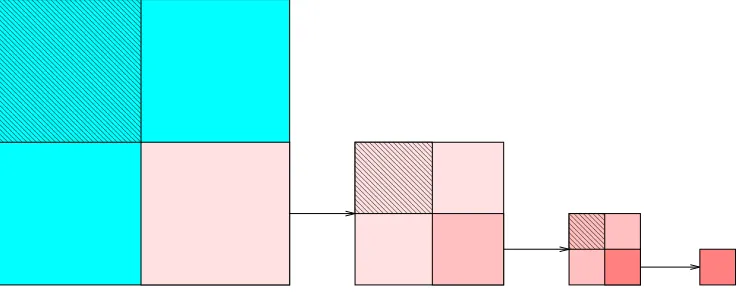
Fig. 2.1.Recursive matrix structure of a4level preconditioner.

2.2. Multilevel preconditioning. For an illustration purpose, we show in Fig. 2.1 the recursive matrix structure of a 4 level preconditioner. Usually, the construction of a multilevel preconditioner consists of two phases. First, at each level the matrix is permuted into a two by two block form, according to some criterion or ordering strategy,

Aα∼PαAαPαT =

Dα Fα

Eα Cα

, (2.1)

wherePαis the permutation matrix andαis the level reference. For simplicity, we denote both the permuted

and the unpermuted matrices byAα. Second, the matrix is decomposed into a two level structure by a block

LU factorization,

Dα Fα

Eα Cα

=

Iα 0

EαDα−1 Iα

Dα Fα

0 Aα+1

, (2.2)

where Iα is the generic identity matrix at level α. Aα+1 =Cα−EαDα−1Fα is the Schur complement matrix,

which forms the reduced system. The whole process, permuting matrix and performing block LU factorization, can be repeated with respect toAα+1 recursively to generate a multilevel structure. The recursion is stopped

when the last reduced systemAL is small enough to be solved effectively.

The preconditioner application process consists of a level by level forward elimination, the coarsest level solution, and a level by level backward substitution. Suppose the right hand side vector b and the solution vectorxare partitioned according to the permutation in (2.1), we have, at each level,

xα=

xα,1

xα,2

, bα=

bα,1

bα,2

.

The forward elimination is performed by solving a temporary vectoryα, i. e., forα= 0,1, . . . ,L −1, by solving

Iα 0

EαD−α1 Iα

yα,1 yα,2 = bα,1 bα,2 , with

yα,1 = bα,1,

(4)

The last reduced system may be solved to a certain accuracy by a preconditioned Krylov subspace iteration to get an approximate solutionxL. After that, a backward substitution is performed to obtain the preconditioning solution by solving, forα=L −1, . . . ,1,0,

Dα Fα

0 Aα+1

xα,1

xα,2

=

yα,1

yα,2

, with

xα,2 = A−α+11 yα,2,

xα,1 = Dα−1(yα,1−Fαxα,2),

wherexα,2 is actually the coarser level solution.

2.3. Multilevel preconditioner based on MSP. A straightforward way to build a multilevel SAI preconditioner is to compute an SAI matrixMα for the submatrix Dα, and to use Mα to substitute D−α1 in

Eq. (2.2). We have

Dα Fα

Eα Cα

≈

Iα 0

EαMα Iα

Dα Fα

0 Aα+1

,

The approximate Schur complement matrix is computed asAα+1 =Cα−EαMαFα. Continue doing this for

Aα+1 at the next level, a multilevel preconditioner based on SAI can be constructed. Correspondingly, the

forward and backward substitutions in the preconditioner application phase change to

yα,1 = bα,1,

yα,2 = bα,2−EαMαyα,1, and

xα,2 = A−α+11 yα,2,

xα,1 = Mα(yα,1−Fαxα,2). (2.3)

BecauseMα is only an approximation toDα−1,Cα−EαMαFα is not the exact Schur complement matrix, but

an approximation of it. The computed value xα according to (2.3) will deviate from the true value, even if

A−α+11 can be computed exactly. The larger the difference betweenMαand D−α1, the more the deviation ofxα

will have. Thus we prefer an accurate SAI ofDα during the construction of the multilevel preconditioner.

Through suitable permutation, it is possible to find aDαwith some special structure so that a sparse inverse

ofDαcan be computed inexpensively and accurately. A (block) independent set strategy is used in [35, 39, 41, 40]

for building the multilevel ILU preconditioners, in whichDα consists of small block diagonal matrices. Thus

an accurate (I)LU factorization can be applied to these blocks independently. An independent set related strategy to find a well-conditionedDαis also used in [49] to construct a multilevel factored SAI preconditioner.

Unfortunately block independent set algorithms may be difficult to implement on distributed memory parallel computers. Most published parallel multilevel ILU preconditioners are two level implementations [27, 37, 43], truly parallel multilevel implementations have been reported only recently [24, 44].

For SAI based multilevel preconditioners, there is no need to exploit independent set ordering to extract parallelism, although a block diagonal matrix is certainly easy to invert [53]. What we want is to form a well-conditionedDα. A diagonally dominant matrix is well-conditioned and may be inverted accurately. This

suggests us to find a Dα matrix with a good diagonal dominance property so that D−α1 can be computed

inexpensively and accurately. In our implementation, at each level we use a diagonal dominance based strategy to force the rows with small size diagonal entries into the next level system and keep the relatively large diagonal entries in the current level. At the next level another well-conditioned subsystem is found by pushing the rows with unfavorable property into its next level system. This diagonal dominance based strategy is more like a divide and conquer strategy. Each time a difficult to solve problem is divided into two parts. One part is easier to solve than the other. We solve the easier part and employ the Schur complement strategy to deal with the other part.

We can improve the approximation of D−1

α by using MSP. At each level, we compute a series of sparse

matrices such that

MαlMαl−1· · ·Mα1≈D−α1, (2.4)

wherel is the number of steps. The corresponding Schur complement matrix can be formed as

Cα−EαMαlMαl−1· · ·Mα1Fα. (2.5)

(5)

Matrix permutation. We give a simple diagonal dominance based strategy to find a well-conditioned Dα

matrix. This can be accomplished by computing a diagonal dominance measure for each row of the matrix based on the diagonal value and the sum of the absolute nonzero values of the row [50], i. e.,ti=|aii|/Pj∈Nz(i)|aij|.

Here Nz(i) is the index set of the nonzeros of theith row. If theith row is a zero row (locally) in a processor, we setti = 0. Then the rows with the largest diagonal dominance measures are permuted to form the upper

block matricesDα.

Letφbe a parameter between 0 and 1, which is referred to as the reduction ratio. We keep thek·φrows with the largest diagonal dominance measures at the current level and letk·(1−φ) rows go to the next level. Whenφis close to 1, the reduced system (next level matrix) will be small. We can maintain load balancing by using the sameφin each processor.

We should also point out that in our implementation, the number of levels is not an input parameter like in the other multilevel methods, e.g., BILUM [39]. The multilevel setup algorithm builds the multilevel structure automatically, usingφas the constraint. One option is to let the construction phase stop when each processor has only 1 unknown. The last reduced system may be easy to solve. But this may generate too many levels.

To improve the performance of the diagonal dominance based permutation, a local pivoting strategy can be used before we compute the diagonal dominance measures. The local pivoting strategy finds the largest entry in each row of the local matrix, and permutes this entry to the main diagonal. So that most of the main diagonal entries in the local matrix will be larger than the offdiagonal entries in the same row. The submatrixDαafter

the diagonal dominance based permutation is more diagonally dominant and better conditioned.

Forward and backward preconditioning. When examining the forward and backward steps in (2.3), we find

that the operation ˜xα = Mαbα appears twice. In exact form, this operation should be xα = D−α1bα. So the

value ˜xα is only an approximation of the true value xα. The more accurately that ˜xα approximates xα, the

better a preconditioner we have. We can improve the computed value ˜xαby a preconditioned GMRES iteration

onMαDαxα=Mαbαand using ˜xα as the initial guess. We call this preconditioning iteration as a forward and

backward preconditioning (FBP) iteration.

Because the reduced systems (Schur complement matrices) are not computed exactly, there is no need to perform many FBP iterations to obtain a very accurate value of ˜xα. A few sweeps are sufficient to make the

approximate inverse ofDα comparably accurate with respect to other parts of the preconditioning matrix.

Schur complement preconditioning. When using MSP to compute the SAI of a matrix, a larger number of

steps will produce a better approximation [48]. The final form of the preconditioner is a multi-matrix form and these matrices are stored individually. The combined storage cost of MSP is not too large if each matrix is sparse. This is one of the advantages of MSP over the standard SAI [48]. When using MSP to generate a multilevel preconditioner, these sparse matrices have to be multiplied out to compute the reduced systemAα+1

as in (2.5). This may result in a dense Schur complement matrix.

A compromise can be reached in this situation by computing two Schur complement matrices with different accuracy by using different drop tolerances [29]. The more sparse one is used as the coarse level system to generate the coarse level preconditioner, and is discarded after serving that purpose. The more accurate and denser Schur complement matrix is kept as a part of the preconditioning matrix and is used in the preconditioner application phase. In our multilevel MSP preconditioner, we use a similar strategy to control the storage cost. Here the two Schur complement matrices are not computed by using different drop tolerances but by using different steps in MSP.

Suppose that MSP generates a series of matrices as in (2.4). We construct the explicit Schur complement matrix (for the reduced system) by using only the first few steps of (2.4), e.g., onlyMα1, we haveCα−EαMα1Fα.

BecauseMα1is usually very sparse according to [48], this Schur complement matrix may be sparse (at least more

sparse than the Schur complement matrix (2.5)) and can be computed inexpensively. In the preconditioning phase, we may use the more accurate Schur complement matrix (2.5) in an implicit form. To further improve the accuracy of the Schur complement solution, we may iterate on the implicit Schur complement matrix (2.5) with the lower level preconditioner. This strategy is called Schur complement preconditioning [51]. During the Schur complement preconditioning phase, we only perform a series of matrix vector products. We can see that if each of these matrices is sparse, the combined storage cost is not too high.

Stored preconditioning matrices. At each level α of the multilevel preconditioner, we should store Eα,

Fα, and the computed MSP matrices MαlMαl−1· · ·Mα1 for the forward and backward substitutions in the

(6)

preconditioning is implemented, the matrixCα should also be kept. Therefore, the sparsity ratio, which is the

storage cost of the preconditioning matrices divided by the storage cost of the original matrix, is at least 1. Some strategies may reduce the storage cost, e.g., the matricesD0,E0,F0andC0do not need to be stored, they

can be recovered by a permutation from the original matrix [51]. In our current prototype implementation, we do not use this strategy. At each Krylov subspace iteration, the permutation to recover these four submatrices may be expensive on distributed memory parallel computers.

4. Experimental Results. We implement our parallel multilevel MSP preconditioner (MMSP) based on the strategies outlined in the previous sections. At each level, we use a diagonal dominance measure based strategy to permute the matrix into a two by two block form. A static sparsity pattern based MSP is used to compute an SAI ofDα. During the preconditioning phase, we perform forward and backward preconditioning

(FBP) iterations to improve the performance of MMSP. The last level reduced system is solved by a GMRES iteration preconditioned by MSP. We use the MSP code developed in [48] to build our MMSP code, which is written in C with a few LAPACK routines [1] written in Fortran. The interprocessor communications are handled by MPI [20]. We conduct a few numerical experiments to show the performance of MMSP. We also compare MMSP with MSP to show the improved robustness and efficiency due to the introduction of the multilevel structure.

The computations are carried out on a 32 processor (750 MHz) subcomplex of an HP superdome (super-cluster) with distributed memory at the University of Kentucky. Unless otherwise indicated explicitly, four processors are used in our numerical experiments.

For all preconditioning iterations, which include the outer (main) preconditioning iterations, FBP iterations, Schur complement preconditioning iterations, and the coarsest level solver, we use a flexible variant of restarted parallel GMRES (FGMRES) [33, 34].

In all tables containing numerical results, “φ” is the reduction ratio; “step” indicates the number of steps used in MSP; “iter” shows the number of outer iterations for the preconditioned FGMRES(50) to reduce the 2-norm residual by 8 orders of magnitude. We also set an upper bound of 2000 for the FGMRES iteration, a symbol “-” in a table indicates lack of convergence; “density” stands for the sparsity ratio; “setup” is the total CPU time in seconds for constructing the preconditioner; “solve” is the total CPU time in seconds for solving the given sparse linear system; “total” is the sum of “setup” and “solve”; “ǫ” is the parameter used in MMSP and MSP to sparsify the computed SAI matrices.

4.1. Test problems. We first introduce the test problems used in our experiments. The right hand sides of all linear systems are constructed by assuming that the solution is a vector of all ones. The initial guess is a zero vector.

Convection-diffusion problem. A three dimensional convection-diffusion problem (defined on a unit cube)

uxx+uyy+uzz+ 1000 (p ux+q uy+r uz) = 0 (4.1)

is used to generate some large sparse matrices to test the scalability of MMSP. Here the convection coefficients are chosen asp=x(x−1)(1−3y)(1−2z), q=y(y−1)(1−2z)(1−2x), r=z(z−1)(1−2x)(1−2y).The Reynolds number for this problem is 1000. Eq. (4.1) is discretized by using the standard 7 point central difference scheme and the 19 point fourth order compact difference scheme [23]. The resulting matrices are referred to as the 7 point and 19 point matrices respectively.

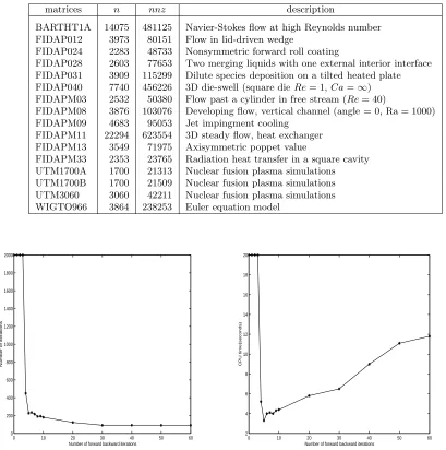
General sparse matrices. We also use MMSP to solve the sparse matrices listed in Table 4.1.

The BARTHT1A matrix is from a 2D high Reynolds number airfoil problem with turbulence modeling. The WIGTO966 matrix comes from an Euler equation model and was supplied by L. Wigton from Boeing. (Both BARTHT1A and WIGTO966 matrices are available from the corresponding author). The FIDAP matrices are extracted from the test problems provided in the FIDAP package [18]. They arise from coupled finite element discretization of Navier-Stokes equations modeling incompressible fluid flows. The UTM matrices are real non-symmetric matrices arising from nuclear fusion plasma simulations in a tokamak reactor. The UTM matrices and the FIDAP matrices can be downloaded from the MatrixMarket of the National Institute of Standards and Technology.1 _{We remark that, based on our experience, most of these matrices are considered difficult to solve}

by standard SAI preconditioners.

1

(7)

Table 4.1

Information about the general sparse matrices used in the experiments (n is the order of a matrix, nnz is the number of nonzero entries).

matrices n nnz description

BARTHT1A 14075 481125 Navier-Stokes flow at high Reynolds number FIDAP012 3973 80151 Flow in lid-driven wedge

FIDAP024 2283 48733 Nonsymmetric forward roll coating

FIDAP028 2603 77653 Two merging liquids with one external interior interface FIDAP031 3909 115299 Dilute species deposition on a tilted heated plate FIDAP040 7740 456226 3D die-swell (square dieRe= 1,Ca=∞) FIDAPM03 2532 50380 Flow past a cylinder in free stream (Re= 40)

FIDAPM08 3876 103076 Developing flow, vertical channel (angle = 0, Ra = 1000) FIDAPM09 4683 95053 Jet impingment cooling

FIDAPM11 22294 623554 3D steady flow, heat exchanger FIDAPM13 3549 71975 Axisymmetric poppet value

FIDAPM33 2353 23765 Radiation heat transfer in a square cavity UTM1700A 1700 21313 Nuclear fusion plasma simulations UTM1700B 1700 21509 Nuclear fusion plasma simulations UTM3060 3060 42211 Nuclear fusion plasma simulations WIGTO966 3864 238253 Euler equation model

0 10 20 30 40 50 60

0 200 400 600 800 1000 1200 1400 1600 1800 2000

Number of forward backward iterations

Number of iterations

0 10 20 30 40 50 60

2 4 6 8 10 12 14 16 18 20

Number of forward backward iterations

CPU time(seconds)

Fig. 4.1. Convergence behavior of MMSP using different number of FBP iterations for solving the UTM1700B matrix

(φ= 0.67,step = 2, ǫ= 0.05,density = 3.48,level = 7). Left: the number of outer iterations versus the number of FBP iterations.

Right: the total CPU time versus the number of FBP iterations.

4.2. Performance of MMSP.

Forward and backward preconditioning. Fig. 4.1 depicts the convergence behavior and the CPU time with

(8)

Table 4.2

Solving the BARTHT1A matrix with different MMSP levels (φ= 0.67,step = 3, ǫ= 0.02).

level size density iter setup solve total 2 4692 5.13 1843 22.5 417.1 439.6 4 524 6.88 238 18.0 71.8 89.8 6 60 6.86 140 17.3 41.8 59.1

8 8 6.86 137 17.3 40.1 57.4

Table 4.3

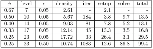
Solving the WIGTO966 matrix with different values ofφ(step = 2).

φ level ǫ density iter setup solve total

0.67 7 0.05 2.61 - 2.1 -

-0.50 10 0.05 5.67 184 3.8 9.7 13.5 0.40 14 0.05 9.03 81 7.8 5.2 13.1 0.33 17 0.05 12.14 45 13.3 3.5 16.8 0.25 23 0.05 17.72 33 26.4 3.1 29.5 0.25 23 0.50 10.74 1083 12.6 86.8 99.4

point out that the optimum value of this parameter may be problem dependent, and 5 FBP iterations may not be the best for all problems.

Reduction ratio and number of levels.. The sizes of the current level matrix and the next level (reduced)

matrix are controlled by the reduction ratioφ. φis an important parameter for deciding the number of levels and influences the performance of MMSP. Here we give some experimental results concerning the reduction ratio and the number of MMSP levels.

The data in Table 4.2 are from solving the BARTHT1A matrix using φ = 0.67. We let the multilevel construction stop when the number of levels reaches a predefined value. The column “size” in the table indicates the size of the last reduced (coarsest) system, which is solved by a preconditioned FGMRES(5) iteration when the 2-norm residual is reduced by a factor of 108_{or the maximum number of 5 iterations is reached.}

It can be seen that a 2 level MMSP, with the last reduced system of 4692 unknowns, needs 1843 iterations and 439.6 seconds to converge. An 8 level MMSP, with the last reduced system of only 8 unknowns, converges in 137 iterations and in 57.4 seconds. In particular, we observe that both the setup time and the solution time are reduced with more levels. The smaller setup time with more levels is due to the fact that a less expensive SAI is constructed for a smaller last level reduced system with more levels.

This experiment indicates that an MMSP with more levels is advantageous for this test problem. In our following experiments, the construction of MMSP stops when there is only one unknown left in each processor. So the number of levels controlled by the reduction ratioφ is−log(1−φ)n, where nis the subproblem size in

each processor. For the same problem, different reduction ratio may result in different number of MMSP levels. Next we use the WIGTO966 matrix to show the influence ofφ value on the performance of MMSP. The results are given in Table 4.3. We can see that whenφ= 0.67, a 7 level MMSP is constructed in 2.1 seconds but does not converge. Whenφ decreases from 0.50 to 0.25, the corresponding number of MMSP levels increases from 10 to 23 and the number of MMSP iterations decreases from 184 to 33, which means that MMSP is more robust when a small φ value is used. Unfortunately, a small φvalue also incurs a large storage cost because more matrices are stored in MMSP.

In the last two rows of Table 4.3, we use the same φ = 0.25 but different ǫ values (0.05 and 0.5). The computed two MMSPs have the same number of levels. The storage cost (density) of the second one is 10.74, compared to 17.72 of the first one. However, the second one needs more iterations (1083) and more solution time (86.8 seconds) to converge. Its performance is worse than that reported in the row 2, where the number of levels is 10, the density is 5.67, and MMSP only needs 184 iterations and 9.7 seconds to converge.

The previous two tests imply that it is not advantageous to set the value ofφto be too large or too small. In the following tests, we useφ= 0.67.

In Table 4.4 we show the diagonal dominance and the 2-norm condition number of the matrices Aα and

Dα at the first four levels of MMSP for the FIDAP031 matrix. “ddiag” in the table is the ratio of the number

(9)

Table 4.4

The diagonal dominance ratio and the condition number of the matrices at each level of MMSP for the FIDAP031 matrix (φ= 0.67,step = 2, ǫ= 0.05,density = 2.48).

Aα Dα

level size ddiag cond size ddiag cond 1 3909 0.05 1.0∗106 2606 0.36 6.3∗104 2 1303 0.06 7.9∗103 868 0.17 62.9 3 435 0.01 5.3∗103 290 0.36 33.59 4 145 0.43 84.79 96 0.81 26.78

Table 4.5

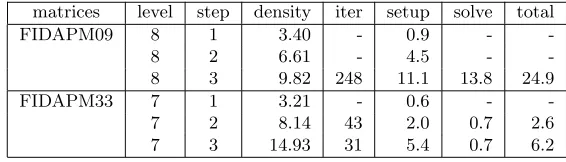
Comparison of MMSP with different MSP steps for solving two FIDAP matrices (φ= 0.67, ǫ= 0.01).

matrices level step density iter setup solve total

FIDAPM09 8 1 3.40 - 0.9 -

-8 2 6.61 - 4.5 -

-8 3 9.82 248 11.1 13.8 24.9

FIDAPM33 7 1 3.21 - 0.6 -

-7 2 8.14 43 2.0 0.7 2.6

7 3 14.93 31 5.4 0.7 6.2

well-conditioned and diagonally dominant matrix Dα can be found at each level by the diagonal dominance

based strategy. E.g., at the first level, the condition number of the original matrix is 1.0∗106 _{and the diagonal}

dominance ratio is 0.05. After the permutation we can get a matrixD1with a condition number 6.3∗104and a

diagonal dominance ratio 0.36. The matrixD1 is easier to solve than the matrixA. This is how the multilevel

preconditioner works. Instead of preconditioning an ill-conditioned matrix directly, it transforms the matrix into some well-conditioned parts and preconditions these matrix parts level by level.

Number of steps. The data in Table 4.5 show the influence of different MSP steps on the performance of

MMSP. For the FIDAPM09 matrix, MMSP does not converges with 1 and 2 MSP steps. It converges with 3 MSP steps in 248 iterations. For the FIDAPM33 matrix, MMSP converges with 2 and 3 MSP steps, but fails in the 1 MSP step case. Just as we expected, a larger number of MSP steps builds a more robust MMSP preconditioner.

Schur complement preconditioning. In Table 4.5, we see that the storage cost of MMSP with 3 MSP

steps is large and the implementation may be impractical in large scale applications. The Schur complement preconditioning strategy may alleviate this problem to some extent [51]. We rerun the two test problems in Table 4.5 using the two Schur complement matrix strategy. The two Schur complement matrix strategy is only implemented at the first level. Here we use the FIDAPM09 matrix as an example to explain how the strategy works. In the setup phase, a 3 step MSP is used to form the SAI ofD1, i. e.,M3M2M1≈D1−1. Then the explicit

Schur complement matrixC1−E1M1F1 is computed as the next level matrix. In the preconditioning phase,

we iterate on the implicit Schur complement matrixC1−E1M3M2M1F1 by FGMRES(50) preconditioned by

the lower level part of MMSP constructed fromC1−E1M1F1. The test results are shown in Table 4.6, where

“step” is the number of MSP steps in the implicit Schur complement matrix. We only allow at most 50 Schur complement preconditioning iterations.

From Tables 4.5 and 4.6 we can see that the two Schur complement matrix strategy reduces the sparsity ratio of MMSP for solving the FIDAPM09 matrix from 9.82 to 4.79. For solving the FIDAPM33 matrix, the sparsity ratio of the 2 MSP step case is reduced from 8.14 to 4.51 and that of the 3 MSP step case is reduced from 14.93 to 6.65. In addition, the setup (construction) time is also reduced to some extent with the two Schur complement matrix strategy. We consider the two Schur complement matrix strategy as an effective way to reduce the memory cost of MMSP. However, the solution time increases because the Schur complement preconditioning strategy utilizes a lot of matrix vector products in the preconditioning phase. We provide the Schur complement preconditioning strategy as an option in our MMSP code in case we have to use a large number of MSP steps for some difficult problems and if the memory cost is more critical than the CPU time.

(10)

Table 4.6

Results of the two Schur complement matrix strategy, compared to Table 4.5.

matrices level step density iter setup solve total

FIDAPM09 8 3 4.79 94 2.5 66.6 69.1

FIDAPM33 7 2 4.51 19 0.7 9.1 9.9

7 3 6.65 15 1.8 7.7 9.5

performance results for solving these matrices. For MMSP we fix ǫ= 0.05 and step = 2. The number in the parentheses of MSP is the number of steps, and the number in the parentheses of MMSP is the number of MMSP levels.

Table 4.7

Comparison of MSP and MMSP for solving a few sparse matrices.

matrices preconditioner ǫ density iter setup solve total FIDAP024 MSP(3) 0.01 4.87 188 14.4 1.8 16.3

MMSP(7) 0.05 3.05 39 0.8 0.6 1.4

FIDAPM08 MSP(3) 0.01 3.28 729 48.3 3.4 51.7

MMSP(8) 0.05 3.02 192 1.1 4.5 5.6

FIDAP012 MSP(-) - - - -

-MMSP(8) 0.05 3.38 57 1.1 1.2 2.3

FIDAP040 MSP(-) - - - -

-MMSP(8) 0.05 3.46 39 4.3 4.0 8.3

FIDAPM03 MSP(-) - - -

-MMSP(7) 0.05 3.35 62 0.8 1.0 1.8

-MMSP(9) 0.05 6.81 200 16.3 85.1 101.4

-MMSP(8) 0.05 3.58 86 1.1 1.7 2.8

UTM1700A MSP(-) - - -

-MMSP(7) 0.05 3.45 145 0.7 1.9 2.6

UTM3060 MSP(-) - - -

-MMSP(8) 0.05 4.02 474 1.0 7.9 8.9

Only 2 of the 9 tested matrices can be solved by MSP. The MMSP can solve these two matrices with smaller sparsity ratios and only 10 percent of the CPU time. In addition, MSP fails to solve the other 7 matrices, which can be solved by MMSP effectively.

Fig. 4.2 shows the convergence behavior of the first 100 MMSP and MSP iterations for solving the FIDAP028 matrix. We can see that MSP reduces the relative residual norm by almost 8 orders of magnitude in 100 iterations. But MMSP reduces the relative residual norm by almost 16 orders of magnitude. From the results of Table 4.7 and Fig. 4.2, we conclude that MMSP is more efficient and more robust than MSP.

4.4. Scalability tests. The main computational costs in MMSP are the matrix-matrix product and matrix-vector product operations. These operations can be performed in parallel efficiently on most distributed memory parallel architectures.

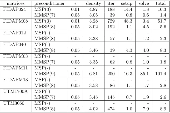
We use the 3D convection-diffusion problem (4.1) to test the implementation scalability of MMSP. The results in Fig. 4.3 are from solving a 7-point matrix with n= 1003_and_nnz_{= 6940000 using different number}

(11)

0 10 20 30 40 50 60 70 80 90 100 10−18

10−16

10−14

10−12

10−10

10−8

10−6

10−4

10−2

100

2−norm relative residual

MSP MMSP

Fig. 4.2. Convergence behavior of MMSP and MSP for solving the FIDAP028 matrix in100iterations (MMSP:density = 2.83, ǫ= 0.05,level = 7,step = 2; MSP:density = 5.34,step = 3, ǫ= 0.005).

4 6 8 10 12 14 16 18 20 22 24 26 28 30 32 50

52 54 56 58 60 62 64 66 68 70 72 74 76 78 80

Number of processors

4 6 8 10 12 14 16 18 20 22 24 26 28 30 32 4

8 12 16 20 24 28

Speedup

Fig. 4.3. Scalability test of MMSP when solving a7point matrix withn= 1003

,nnz= 6940000 (ǫ= 0.1,step = 2,level =

10,density = 2.03). Left: the number of MMSP iterations versus the number of processors. Right: the speedup of MMSP as a

function of the number of processors.

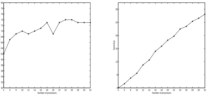
In Fig. 4.4, the scaled scalability of MMSP is tested by solving a series of 19-point matrices. We try to keep the number of unknowns in each processor to be approximately 253_{. When we change the number of processors,}

the problem size increases at the same time. To be comparable, we also give the scaled scalability of MSP in the same figure. The parameters used are step = 1,level = 10, ǫ= 0.1 for MMSP, and step = 2, ǫ= 0.05 for MSP. From Fig. 4.4, We find that MMSP shows better scaled scalability than MSP for this test problem. The behavior of MMSP are more stable than that of MSP.

5. Summaries. We have developed a class of parallel multilevel sparse approximate inverse (SAI) precon-ditioners based on MSP for solving general sparse matrices. A prototype implementation is tested to show the robustness and computational efficiency of this class of multilevel preconditioners.

(12)

5 10 15 20 25 30 0

30 60 90 120 150

MSP MMSP

5 10 15 20 25 30

0 10 20 30 40 50 60 70 80

CPU time(seconds)

MSP MMSP

Fig. 4.4. Scaled scalability test of MMSP and MSP for solving a series of19point matrices withn≈253 in each processor.

Left: the number of iterations versus the number of processors. Right: the total CPU time versus the number of processors.

The number of MMSP levels influences the convergence and storage cost of the preconditioner. A large number of levels results in a fast MMSP preconditioner with a high storage cost. A small number of levels results in an inexpensive preconditioner with a low storage cost. The same statement is valid with respect to the number of MSP steps used at each level of MMSP. We can use a two Schur complement matrix strategy to reduce the storage cost.

Compared with MSP, MMSP is more robust and costs less to construct. The scalability of MMSP seems to be good. But the convergence of MMSP may be affected by the number of processors employed, due to the local matrix reordering implemented to enhance the factorization stability.

Acknowledgements. Kai Wang’s research work was funded by the U. S. National Science Foundation under grants CCR-9902022 and ACI-0202934. Jun Zhang’s research work was supported in part by the U.S. National Science Foundation under grants CCR-9902022, CCR-9988165, CCR-0092532, and ACI-0202934, by the U. S. Department of Energy Office of Science under grant DE-FG02-02ER45961, by the Japanese Research Organization for Information Science & Technology, and by the University of Kentucky Research Committee. Chi Shen’s research work was funded by the U.S. National Science Foundation under grants CCR-9902022 and CCR-0092532.

REFERENCES

[1] E. Anderson, Z. Bai, C. Bischof, J. Demmel, J. Dongarra, J. Du Croz, A. Greenbaum, S. Hammarling, A. McKenney, S. Ostrouchov, and D. Sorensen,LAPACK Users’ Guide. SIAM, Philadelphia, PA, 2 edition, 1995.

[2] O. Axelsson,Iterative Solution Methods. Cambridge Univ. Press, Cambridge, 1994.

[3] R. E. Bank and C. Wagner,Multilevel ILU decomposition. Numer. Math., 82(4):543–576, 1999.

[4] S. T. Barnard, L. M. Bernardo, and H. D. Simon,An MPI implementation of the SPAI preconditioner on the T3E. Int. J. High Perf. Comput. Appl., 13:107–128, 1999.

[5] R. Barrett, M. Berry, T. F. Chan, J. Demmel, J. Donato, J. Dongarra, V. Eijkhout, R. Pozo, C. Romine, and H. van der Vorst, Templates for the Solution of Linear Systems: Building Blocks for Iterative Methods. SIAM Publications, Philadelphia, PA, 1993.

[6] M. W. Benson and P. O. Frederickson,Iterative solution of large sparse linear systems arising in certain multidimensional

approximation problems. Utilitas Math., 22:127–140, 1982.

[7] M. W. Benson, J. Krettmann, and M. Wright,Parallel algorithms for the solution of certain large sparse linear systems.

Int. J. Comput. Math., 16:245–260, 1984.

[8] M. Benzi and M. Tuma, A sparse approximate inverse preconditioner for nonsymmetric linear systems. SIAM J. Sci. Comput., 19(3):968–994, 1998.

(13)

[10] E. F. F. Botta and F. W. Wubs, Matrix renumbering ILU: an effective algebraic multilevel ILU preconditioner for sparse

matrices. SIAM J. Matrix Anal. Appl., 20(4):1007–1026, 1999.

[11] T. F. Chan and V. Eijkhout, ParPre: a parallel preconditioners package reference manual for version 2.0.17. Technical Report CAM 97-24, Department of Mathematics, UCLA, Los Angeles, CA, 1997.

[12] E. Chow, A priori sparsity patterns for parallel sparse approximate inverse preconditioners. SIAM J. Sci. Comput., 21(5):1804–1822, 2000.

[13] E. Chow, Parallel implementation and practical use of sparse approximate inverse preconditioners with a priori sparsity

patterns. Int. J. High Perf. Comput. Appl., 15:56–74, 2001.

[14] E. Chow and Y. Saad,Approximate inverse preconditioners via sparse-sparse iterations.SIAM J. Sci. Comput., 19(3):995– 1023, 1998.

[15] J. D. F. Cosgrove, J. C. Diaz, and A. Griewank,Approximate inverse preconditionings for sparse linear systems. Int. J. Comput. Math., 44:91–110, 1992.

[16] I. S. Duff and G. A. Meurant, The effect of reordering on preconditioned conjugate gradients. BIT, 29:635–657, 1989. [17] A. C. N. van Duin, Scalable parallel preconditioning with the sparse approximate inverse of triangular matrices. SIAM J.

Matrix Anal. Appl., 20:987–1006, 1999.

[18] M. Engelman,FIDAP: Examples Manual, Revision 6.0. Technical report, Fluid Dynamics International, Evanston, IL, 1991. [19] N. I. M. Gould and J. A. Scott, Sparse approximate-inverse preconditioners using norm-minimization techniques. SIAM

J. Sci. Comput., 19(2):605–625, 1998.

[20] W. Gropp, E. Lusk, and A. Skjellum, Using MPI: Portable Parallel Programming with the Message-Passing Interface. MIT, Boston, 2 edition, 1999.

[21] M. Grote and T. Huckle, Parallel preconditioning with sparse approximate inverses. SIAM J. Sci. Comput., 18:838–853, 1997.

[22] M. Grote and H. D. Simon, Parallel preconditioning and approximate inverse on the Connection machines. In R. F.

Sincovec, D. E. Keyes, M. R. Leuze, L. R. Petzold, and D. A. Reed, editors,Proceedings of the Sixth SIAM Conference

on Parallel Processing for Scientific Computing, pages 519–523, Philadelphia, PA, 1993. SIAM.

[23] M. M. Gupta and J. Zhang,High accuracy multigrid solution of the 3D convection-diffusion equation.Appl. Math. Comput., 113(2-3):249–274, 2000.

[24] G. Karypis and V. Kumar,Parallel threshold-based ILU factorization. Technical Report 96-061, Department of Computer Science, University of Minnesota, Minneapolis, MN, 1996.

[25] L. Y. Kolotilina, Explicit preconditioning of systems of linear algebraic equations with dense matrices. J. Soviet Math., 43:2566–2573, 1988.

[26] V. Kumar, A. Grama, A. Gupta, and G. Karypis, Introduction to Parallel Computing. Benjamin/Cummings Pub. Co., Redwood City, CA, 1994.

[27] Z. Li, Y. Saad, and M. Sosonkina, pARMS: a parallel version of the algebraic recursive multilevel solver. Technical Report UMSI 2002-100, Minnesota Supercomputer Institute, University of Minnesota, Minneapolis, MN, 2001.

[28] J. A. Meijerink and H. A. van der Vorst, An iterative solution method for linear systems of which the coefficient matrix

is a symmetric M-matrix. Math. Comp., 31:148–162, 1977.

[29] G. Meurant, A multilevel AINV preconditioner. Numer. Alg., 29(1-3):107–129, 2002.

[30] N. M. Nachtigal, S. C. Reddy, and L. N. Trefethen, How fast are nonsymmetric matrix iterations? SIAM Matrix Anal. Appl., 13(3):778–795, 1992.

[31] K. Nakajima and H. Okuda, Parallel iterative solvers with localized ILU preconditioning for unstructured grids on

work-station clusters. Int. J. Comput. Fluid Dynamics, 12:315–322, 1999.

[32] A. Reusken, On the approximate cyclic reduction preconditioner.SIAM J. Sci. Comput., 21(2):565–590, 1999. [33] Y. Saad,A flexible inner-outer preconditioned GMRES algorithm. SIAM J. Sci. Statist. Comput., 14(2):461–469, 1993. [34] Y. Saad, Parallel sparse matrix library (P SPARSLIB): The iterative solvers module. InAdvances in Numerical Methods

for Large Sparse Sets of Linear Equations, volume Number 10, Matrix Analysis and Parallel Computing, PCG 94, pages 263–276, Yokohama, Japan, 1994. Keio University.

[35] Y. Saad, ILUM: a multi-elimination ILU preconditioner for general sparse matrices. SIAM J. Sci. Comput., 17(4):830–847, 1996.

[36] Y. Saad, Iterative Methods for Sparse Linear Systems. PWS Publishing, New York, NY, 1996.

[37] Y. Saad and M. Sosonkina, Distributed Schur complement techniques for general sparse linear systems. SIAM J. Sci. Comput., 21(4):1337–1356, 1999.

[38] Y. Saad and B. Suchomel,ARMS: an algebraic recursive multilevel solver for general sparse linear systems.Numer. Linear Alg. Appl., 9(5):359–378, 2002.

[39] Y. Saad and J. Zhang, BILUM: block versions of multielimination and multilevel ILU preconditioner for general sparse

linear systems. SIAM J. Sci. Comput., 20(6):2103–2121, 1999.

[40] Y. Saad and J. Zhang,BILUTM: a domain-based multilevel block ILUT preconditioner for general sparse matrices.SIAM J. Matrix Anal. Appl., 21(1):279–299, 1999.

[41] Y. Saad and J. Zhang, Diagonal threshold techniques in robust multi-level ILU preconditioners for general sparse linear

systems. Numer. Linear Algebra Appl., 6(4):257–280, 1999.

[42] Y. Saad and J. Zhang, Enhanced multilevel block ILU preconditioning strategies for general sparse linear systems. J. Comput. Appl. Math., 130(1-2):99–118, 2001.

[43] C. Shen and J. Zhang,Parallel two level block ILU preconditioning techniques for solving large sparse linear systems.Paral. Comput., 28(10):1451–1475, 2002.

[44] C. Shen, J. Zhang, and K. Wang,Distributed block independent set algorithms and parallel multilevel ILU preconditioners. Technical Report No. 358-02, Department of Computer Science, University of Kentucky, Lexington, KY, 2002.

(14)

[46] B. Smith, W. D. Gropp, and L. C. McInnes, PETSc 2.0 user’s manual. Technical Report ANL-95/11, Argonne National Laboratory, Argonne, IL, 1995.

[47] K. Wang, S. B. Kim, J. Zhang, K. Nakajima, and H. Okuda,Global and localized parallel preconditioning techniques for

large scale solid Earth simulations.Future Generation Comput. Systems, 19(4):443–456, 2003.

[48] K. Wang and J. Zhang,MSP: a class of parallel multistep successive sparse approximate inverse preconditioning strategies.

SIAM J. Sci. Comput., 24(4):1141–1156, 2003.

[49] K. Wang and J. Zhang, Multigrid treatment and robustness enhancement for factored sparse approximate inverse

precon-ditioning.Appl. Numer. Math., 43(4):483–500, 2002.

[50] J. Zhang,A multilevel dual reordering strategy for robust incomplete LU factorization of indefinite matrices.SIAM J. Matrix Anal. Appl., 22(3):925–947, 2000.

[51] J. Zhang, On preconditioning Schur complement and Schur complement preconditioning. Electron. Trans. Numer. Anal., 10:115–130, 2000.

[52] J. Zhang, Preconditioned Krylov subspace methods for solving nonsymmetric matrices from CFD applications. Comput. Methods Appl. Mech. Engrg., 189(3):825–840, 2000.

[53] J. Zhang,Sparse approximate inverse and multilevel block ILU preconditioning techniques for general sparse matrices.Appl. Numer. Math., 35(1):67–86, 2000.

[54] J. Zhang, A class of multilevel recursive incomplete LU preconditioning techniques. Korean J. Comput. Appl. Math., 8(2):213–234, 2001.

[55] J. Zhang, A sparse approximate inverse technique for parallel preconditioning of general sparse matrices. Appl. Math. Comput., 130(1):63–85, 2002.

Edited by: L. Brugnano.

Received: November 7, 2003.