ISSN: 2146-4138 www.econjournals.com
819
An Econometric Estimation and Prediction of the Effects of Nominal
Devaluation on Real Devaluation: Does the Marshal-Lerner (M-L)
Assumptions Fits in Nigeria?
Abdulkadir Abdulrashid Rafindadi Department of Accounting, Usmanu Danfodiyo University, Sokoto, Nigeria. Email: [email protected]
Zarinah Yusof
Department of Economics, University of Malaya, Kuala Lumpur, Malaysia. Email: [email protected]
ABSTRACT: Nigeria has been depending on oil as its major export commodity for decades leading to the neglect of other vital economic resources. This situation led to massive unemployment as a result of an undiversified economic system, which in turn created an alarming paucity of external accruals to finance the lingering poverty level of the country. Similar to this, several economic indexes and researchers have been pointing out delusive and inconclusive growth attainment of the country which has not impacted positively on the populace. It is against this backdrop that this study aims to re-investigate whether nominal effective exchange rate could lead to real effective exchange rate and if this can be a synergistic strategy towards spurring competitive trading relationship between Nigeria and the rest of the globe. To ensure this, we use a quarterly time series data from 1971QI-2012QVI, and applied the traditional and structural break unit root tests; the Bayer-Hanck cointegration approach and the VECM-Granger causality test. The findings of the study confirmed that nominal effective exchange rate leads to real effective exchange rate and inflation exerts positive impact on real effective exchange rate in Nigeria. In addition, the study found that real effective exchange rate has positive impact on nominal effective exchange rate, but inflation declines it. The causality analysis, on the other hand, revealed that there is feedback effect between real and nominal effective exchange rates, between nominal effective exchange rate and inflation and between inflation and real effective exchange rate. This finding suggests that there are crystal avalanche of competitive opportunities for the country to jettison all its economic vices and move progressively in international trade with minimal hurdles, thus fitting in with the Marshall-Lerner assumption (M-L).
Keywords: Marshall-Lerner; devaluation; exchange rates; cointegration JEL Classifications: C2; C5; F1; G0
1. Introduction
820 Adewuyi (2011), made Ozurumba and Chigbu (2013) to argue that crude oil is an exhaustible asset which makes it unreliable for sustainable development. In a related development which compounded on the above findings, Rafindadi and Yusof (2014) in their recent study discovered that M3, bank assets, fixed capital formation, trade and private sector contribution in Nigeria have an insignificant contribution to the country’s GDP. Following to these developments, the authors argued that it is most likely that the country may face prolonged macroeconomic volatility due to the absence of strong exogenous risk cushioning effects, chaotic and unfavorable investment climate, high rise in unemployment and persistent exchange rate instability. In addition to this, key macroeconomic variables have been pointing an unfavourable direction to the countries’ economic growth prospects. For instance inflationary rate was discovered to be at the rate of 16% in 1971 rising to an unprecedented high level up to 72.84% in 1995, down to 13.72%, 10.84% and 12.9% in 2010, 2011 and 2012, respectively. In the international trading perspective, Nigeria’s export was reported to be $2,152 billion in 1997 while its import was $14,691.6 billion, thus creating a deficit of $12,539.6 in the same year. Similar trend occurred in 1994 when exports were$5,349 billion, and imports were valued at $120,439.2 leaving a deficit of $115,090 billion in the same year. The situation worsened in 2009 when trade deficit amounted to $366,965 billion, and inflation was 56% in 1988 and 72.8% in 1995 and subsequently dropped to 6.6% in 1999 and 10.3% in 2012. This signifies that import items are rising due to increase in domestic demand. These situations simply lead to the widening of the country’s trade deficit. As a consequence, the country’s balance of payments deteriorated tremendously in those periods.
Advancing the significance of international trade, McTeer (2008) asserted that a significant rise in international trade volume benefit the general standard of living of a country by curving unemployment, diversification in revenue earnings, exploitation of national resources endowment, exchange rate provision, enhancement of the value of a national currency and help in averting exogenous shock.The author continued to assert that where trade grows significantly, it aids in economic leadership of the country regionally or even at the global level.It is in reference to this that this study aims to investigate the relationship between nominal effective exchange rate and real effective exchange rate in Nigeria. In this study, considering the rising trend of inflation in Nigeria we incorporate inflation as additional variable to the determination of nominal and real effective exchange rates. This is in order to explore more on the assertion made by Bahmani-Oskooee (1998) where the author argued that moderate inflation eats up the unfavorable impacts of nominal devaluation. Following the introduction in section I, section II of the paper will provide an overview of theoretical and empirical review of the literature. Section III will be on the conceptual framework of the study and section IV discusses the data, methodology and model specification. Section V presents the results and discussions, and section VI concludes and makes some recommendations to policy implications.
2. Theoretical and Empirical Review
821 The ground breaking research of Vaubel (1976) was among the key supporters of currency devaluation. In his empirical arguments, the author established that devaluation provides a significant avenue for international trading competitive advantage, and also help in raising internal efficiencies. From this development, Vaubel (1976) encouraged countries to adopt currency devaluation if they are aiming to achieve full and progressive economy. In the same line of development, Connolly and Taylor (1976, 1979); Bruno, (1978) and Edwards (1988, 1994) find that nominal devaluation results in real devaluation, but only in the short to medium term. For this reason, the authors unanimously, recommend that countries should avoid making devaluation a long term strategy in addressing the problems of balance of payments issues.
With reference to the expenditure switching mechanism theory and the empirical finding of Vaubel, (1976), Nigeria among a group of other countries implemented a system of mixed exchange rate regime which enabled the economy to efficiently distribute resources and remedy the international balance of payments problems until when it was later on abandoned. Bahmani-Oskooee and Mirzai (2000) studied the various probable variations resulting from the implementation of the real effective exchange rate by applying the KPSS test. The study concluded that PPP exists in the majority of developing economies. Subsequently, Bahmani-Oskooee and Miteza (2002) in a further follow up study utilized the error-correction model to examine the importance of the relationship between nominal effective exchange rate and real effective exchange rate in the long run and the short run. The authors used the data set of developing countries, including Pakistan. The findings of the study revealed that nominal devaluation results in real devaluation with minor variations in the values of the variables particularly in the case Pakistan from 1971-1997.
With reference to this finding, devaluation was re-admitted as a mechanism by numerous developing countries to resolve difficulties in balance of payments. To validate this finding and in a further follow up studies, Kent and Naja (1998) found that nominal devaluation results in progressively real devaluation as a nation transfers to a flexible exchange rate system. However, their result with regards to Pakistan was contradictory. Responding to Kent and Naja (1998) Bahmani-Oskooee and Kutan (2008) argued that the results of the previous authors are precarious upon factors such as the level of economic growth, the political climate, the governments’ serious commitment and other economic policies.
In another line of theoretical argument from the Keynesian school of thought it was established that devaluation has positive impacts on output. Notwithstanding this, the monetarists, on their own side, maintained the view that the benefits of devaluation can be traced solely in the short-run and that any long-short-run effects could be negligible. The proponents of this theory continue to maintain their view point that developing continents should not exert persistent pressure on their national currencies; otherwise, the end result may be quite severe. Recently, the comparative value of devaluation in developing countries has been under close scrutiny by the new structuralist economists. They contend that, in the industrialised countries, the position of the exchange rate is market driven. From this perspective, the envisaged benefit of devaluation is obvious. However, in a situation where it is artificially induced it will yield to adverse result.
822 devaluation has a contractionary effect and devaluation diminishes supply at a much more rapid rate as aggregate demand rises.
Notwithstanding all the above arguments yet, the recent findings by Ratha (2010) in India showed that, devalued currency is beneficial for economic growth, exports and trade balance. However, Adam, et al. (2010) asserted that there is no evidence of any link between devaluation of Taka and export revenue in Bangladesh. Similar line of argument were also maintained in the six main economies of Latin America, as studied by Mejı´a-Reyesab et al. (2010) where they concluded that devaluation has a contractionary effect. In another development, Guglielmo et al. (2012) while examining the Marshall-Lerner (ML) condition for the Kenyan economy established that a moderate devaluation of the Kenyan shilling created a stabilizing influence on the balance of payment through the current account without the need for high interest rate re-adjustment and this enhanced the international trading competitive abilities of the country. Contrary to findings of Guglielmo, et al.
(2012), Rafindadi and Yusof (2013) in their empirical research established that the financial development of the Kenyan economy has no significant contribution to the country’s economic growth. This surprising facts may be seen that the effects of the moderate devaluation has not yet impacted on the country’s economic system and that something concrete need to be done.
It is following to this recent study by Guglielmo et al. (2012) and the rising mixed results obtained by authors that this study was motivated to use the latest econometric methodology and re-investigate whether nominal effective exchange rate could lead to real effective exchange rate and to assess the position of the rising inflationary trend in the country Nigeria. The study will equally investigate if this can allow for a synergistic approach towards spurring competitive trading relationship between Nigeria and the rest of the globe?Additionally could the findings of this research fit in with the Marshal-Larner assumptions?
3. Theoretical Framework
The theoretical framework of this study is based on the Marshall-Lerner condition, and the following derivations were obtained from Stern (1973). In that derivation, the author identified trade balance in foreign currency term to follow the outlined definition:
f fx fm
B p Xp M ... (1)
However, when a country devalued its domestic currency (currency depreciation), this leads to:
( ) ( )
f fx fx fx fx
B p X X p p M M p
... (2)
In line with the above, we continue to accommodate the value of export and import by defining each under the following conditions:
fx fx
V p X………foreign value of exports…….... (3)
fx fx
V p M ……….…..foreign value of imports…...… (4) By rearranging and substituting the above equations into equation (2) we have:
fx fm
f fx fm
fx fm
p
p
X
M
B
V
V
X
p
M
p
……….... (5)
From the above equation, we can then continue to invoke the elasticity’s of demand and supply of import and export. In this equation we apply the negative demand elasticity’s to allow us to have a positive equation as follows:
x
fx
fx
X X e
p p
823 x fx fx X X p p
foreign export demand elasticity…. (7)
m fm fm M M e p p
foreign import supply elasticity….. (8)
m fm fm M M p p
home import demand elasticity…. (9)
In the light of the above, it is expected that foreign currency and home currency should relate as a result of the ensuing exchange rate r,and this will us to have:
fm km
p p r
……….……… (10)
Next to the above, we assume home currency to be devaluated by a proportion of k, and this will make the home currency to be worth r(1-k) unit of foreign currency, as a result of this
development, the level of price changes can be seen as follows:
( ) (1 )
fm km km km
p p p p r k ……… (11)
( ) (1 )
fm km km km
p p p r k p r
………..…. (12)
km km km km km
p
p r
p rk
p rk
p r
……….... (13)km km km km
p
p r
p r
p rk
……….…… (14)(1
)
fm km fm kmp
p
k
k
p
p
……….………….…. (15)(1
)
fx kx fx kxp
p
k
k
p
p
………... (16)From our definition of elasticity and substituting equation (6)-(9) into equation (15)-(16) will allow us to have the following:
kx kx x kx
p
p
X
e
X
p
………..………. (17)1 km x km p X e k p X k ………..… (18) 1 (1 ) x x x
X X k
824 (1 ) (1 ) x x x X k e K X e k
……… (20)(1
)
x x x xke
X
X
e
k
……….……..…... (21)(1
)
fx x
fx x x
p
ke
p
e
k
……….…………. (22)(1
)
m m
m x
ke
M
M
e
k
……….………… (23)(1
)
fm m
fm m m
p
k
p
e
k
……….……. (24)To determine the respective changes in the foreign currency value of continental trade balance on the basis of its respective demand and supply elasticity’s we substitute between equation (21) to equation (24) into equation (5), and that will provide us with the following result:
( 1) ( 1)
(1 ) (1 )
x x m m
f fx fm
x x m m
e e
B k V V
e k e k
…… (25)In the above analysis, we further assume that the magnitude of the devaluation in K is meager then we can re-write the equation as follows:
1 (1/
)
1
1 (
/
)
(
/
) 1
m m
x
f fx fm
x x x x
e
B
V
V
e
e
………….. (26)The last equation above provide an explanation on what happen in a situation where prices of goods and services are fixed in sellers currency; the equation, therefore, inform us that the supply elasticity will be infinite elastics. This is commonly known as the Bikerdike-Robinson-Metzler condition (BRM). This is as expressed below:
x m
e
e
………….… (27) From this situation, we will have( 1) ( )
f fx x fm m
B V
V
….. (28)
In the above situation when balanced trade and foreign currency value of exports are equal to the foreign currency value of import then this translate into the following equation:
/ 1
fx fm
V V ………….….. (29)
This condition will undoubtedly increase the international trade balance thus leading to:
0
f
B
……… (30)
Following to the above, what if the sum of the import and export demand elasticity’s is greater than or equal to 1.
x m
……… (31)825
/
fx fm
V V ………. (32)
This condition will undoubtedly increase the foreign currency value such as in:
f
B
……….... (33)
In this respect if the total of export demand elasticity and the weighted import demand elasticity are more than 1, in this respect, consider where the weight is the foreign currency value of the total import then divide by foreign currency value of exports thus:
fm
x x
fx
V
V
………… (34)From the above situation if we invoke our Marshall-Lerner assumption of trade balance being in surplus, this situation yield an insufficient condition. As a result going back to our initial assumptions of trade deficit becomes essential that is where we have:
/
fx fm
V V ……… (35)
Then the following will happen:
f
B
……… (36)
Particularly if:
fm
x m
fx
V
V
…………. (37)In the above equation, the M-L assumption will become the final condition considering the weighted import demand elasticity which can be significantly large or small.
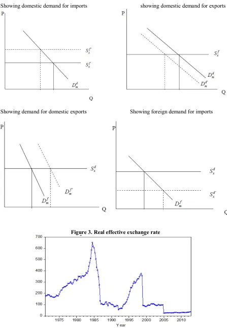
826 Figure 2. graphical representation of Marshall-Lerner conditions for domestic currency and foreign currency.
Showing domestic demand for imports showing domestic demand for exports
Showing demand for domestic exports Showing foreign demand for imports
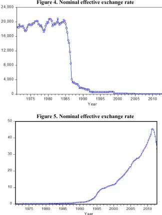
827 Figure 4. Nominal effective exchange rate
Figure 5. Nominal effective exchange rate
4. Model Construction and Data Collection
The prime objective of the present study is to reinvestigate whether nominal effective exchange rate leads to real effective exchange rate in the case of Nigeria. In doing so, and considering the high rates of inflation in the country we have incorporated inflation (consumer price index) as additional determinant of both real and nominal effective exchange rates in order to assess its position in enhancing the favourability or otherwise of the real effective exchange rate in Nigeria. The empirical equations of both models are given as follows:
i t t
t
NER
INF
RER
ln
ln
ln
1 2 2 …………. (38)lnRERt= 1 + 2lnNERt + 2lnINFt+ I ……….. (39)
Where,
RER
tis the real effective exchange rate,NER
tis the nominal effective exchange rate,INF
is the inflation rate proxied by the consumer price index and
iis the error term which is assumed to be normally distributed. The data of the study covers the period of 1971QI-2012QIV, and these were obtained from the Central Bank of Nigeria (CBN). In addition to this, the data on Nigeria’s inflationary rate was also obtained from the Central Bank of Nigeria.4.1. Bayer-Hanck Cointegration Approach
828 Following to this, conflicting results will be common. In this circumstance, it is difficult to obtain consistent results because one cointegration test rejects the null hypothesis but another accepts it. To reduce the effects of this situation Bayer and Hanck (2012) developed a new cointegration technique which combines all non-cointegrating tests to obtain consistent and reliable cointegration results. This cointegration test provides efficient estimates by ignoring the nature of multiple testing procedures. This suggests that the application of non-combining cointegration tests provides robust and efficient results compared to individual t-test or system based test. In his econometric modeling, Bayer and Hanck (2012) followed Fisher (1932) by combining the statistical significance level i.e. p-values of single cointegration analysis as follows:
)]
ln(
)
(
[ln
2
P
EGP
JOHJOH
EG
……….. (40))]
ln(
)
ln(
)
ln(
)
(
[ln
2
P
EGP
JOHP
BOP
BDMBDM
BO
JOH
EG
…… (41)The probability values of different individual cointegration tests such as Engle-Granger, (1987); Johansen, (1995); Boswijik, (1994) and Banerjee, Dolado and Mestre (1998) are shown by
BO JOH
EG
P
P
P
,
,
andP
BDMrespectively. To take decision whether cointegration exists or not between the variables, we follow Fisher statistic. We may conclude in favor of cointegration by rejecting the null hypothesis of no cointegration once critical values generated by Bayer and Hanck are less than calculated Fisher statistics and vice versa.4.2 The VECM Granger Causality Approach
We apply the vector error correction model (VECM) Granger-causality test to examine the direction of the causal relationship between the variables. This method is followed by the two steps of Engle and Granger (1987) and employed to investigate the long-run and short-run dynamic causal relationships. The first step estimates the long-run parameters in equations (1-2) this was done in order to obtain the residuals corresponding to the deviation from equilibrium. The second step estimates the parameters related to the short-run adjustment. The resulting equations are used in conjunction with Granger causality testing:
t t t t t t t i i i i i i i i i p i t t tECT
INF
NER
RER
b
b
b
b
b
b
b
b
b
L
a
a
a
INF
NER
RER
L
3 2 1 1 1 1 1 33 32 31 23 22 21 13 12 11 1 3 2 1ln
ln
ln
)
1
(
ln
ln
ln
)
1
(
(42)Where,
j(j=1,2,3) represents the time-invariant constant; c (c = 1,…,d) is the optimal lag lengthdetermined by the minimization of AIC criterion; (1−L) is the lag operator;
ECT
t1 is the lagged residual;
j (j=1,2,3) is the adjustment coefficient; and
j t, (j=1,2,3) is the disturbance term assumed to be uncorrelated with zero means. The statistical significance of the coefficient of lagged error term i.e.ECT
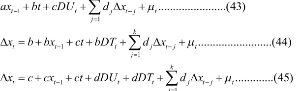
t1 shows the long run causal relationship between the variables. The short run causality is shown by statistical significance of F-statistics using Wald-test by incorporating differences and lagged differences of independent variables in the model. Moreover, the joint significance of the lagged error term with differences and lagged differences of independent variables provides joint long-and-short runs causality. For example, Granger causality running from nominal effective exchange rate to real effective exchange rate if b12,i 0iand from the opposite side it is b21,i 0i.829 econometric mechanism that eliminate the observed bias in other tests and to equally allow for the accommodation of a single structural break point at level form. The Zivot-Andrew (1992) test with structural breaks as used in this study can be tested using the following econometric models:
1
1
1
1
1
1
...(43)
...(44)
...(45)
k
t t j t j t
j
k
t t t j t j t
j
k
t t t t j t j t
j
ax
bt
cDU
d
x
x
b bx
ct
bDT
d
x
x
c cx
ct
dDU
dDT
d
x
Where DUt denotes the dummy variable, and it provides the shifting possibilities of the mean in each point while DTt is a shift in the trending variable.
DU
t
1...
if
t
TB
0...
if
t
£
TB
andDU
t
t
TB
...
if
.
t
TB
0...
if
.
t
£
TB
……….(46)
The null hypothesis of unit root break date is c = 0 which indicates that series is not stationary with a drift not having information about structural break stemming in the series while c <0 hypothesis implies that the variable is found to be trend-stationary with one unknown time break. Zivot-Andrews unit root test fixes all points as potential for possible time break and does estimation through regression for all possible structural breaks successively. Then, this unit root test selects that time break that decreases one-sided t-statistic to test cˆ(= c - 1) = 1. Zivot- Andrews intimate that in the presence of end points, asymptotic distribution of the statistics is diverged to infinity point. It is necessary to choose a region where end points of sample period are excluded. Further, Zivot-Andrews suggested the trimming regions i.e. (0.15T, 0.85T) are followed.
5. Presentation and Interpretation of Results
Primarily, we have to test for the unit root properties of the variables, in doing so, we choose the combining non-cointegration test to examine whether cointegration between the variables exist. In addition to this, it requires that all the series should be stationary at I(1). If none of the variables are stationary, under or beyond the order of integration then computation process for cointegration becomes useless. To solve this problem, we apply ADF and PP unit root tests to test the integrating properties of the variables. The results of ADF and PP unit root tests are reported in Table-1. The results reveal that all the variables have unit root problem (with intercept and trend). However, at first difference, we found all the variables to be stationary. This shows that all the series are integrated at I(1). The same inference is drawn from PP unit root test.
Table 1. Unit Root Testing
Variables ADF Unit Root Test PP Unit Root Test T-statistics Prob.-values T-statistics Prob.-values
t
NER
ln
-2.1875 (4) 0.4930 -2.3197 (3) 0.4206t
RER
ln
-2.6496 (4) 0.2592 -2.3398 (3) 0.4098t
CPI
ln
-0.6574 (2) 0.9739 -0.7395 (9) 0.9679t
NER
ln
-5.2291 (4)* 0.0001 -11.7370 (6)* 0.0000t
RER
ln
-4.8782 (4)* 0.0004 -11.6040 (3)* 0.0000t
CPI
ln
-3.4964 (2) ** 0.0430 -3.4134 (3) ** 0.0530830 The problem with traditional unit root tests such as ADF and PP is that these tests do not accommodate information about structural break stemming in the series. These structural breaks may be a source of unit root problem and make the series non-stationary. The ADF and PP unit root tests over reject the null hypothesis once it is true and vice versa particularly in the presence of structural breaks. To manage the situation of structural breaks, we applied the Zivot-Andrews unit root test that accommodates the information about single unknown structural break in the series. The results are shown in Table-2. We find that the nominal real effective exchange rate (
ln
NER
t), the real effective exchange rate (ln
RER
t) and the consumer price index (ln
CPI
t) are non-stationary in the presence of structural breaks. The structural breaks such as 1986Q2, 2005Q1 and 1991Q2 are found in the nominal real effective exchange rate, the real effective exchange rate) and the consumer price index, respectively. At first difference, the nominal real effective exchange rate (ln
NER
t), the real effective exchange rate (ln
RER
t) and the consumer price index are found to be stationary. This shows that variables have a unique order of integration. This leads us to apply the Bayer and Hanck, (2012) cointegration approach to examine the long-run relationship between the variables.Table 2. Zivot-Andrews Unit Root Test
T-statistic Time Break
t
NER
ln
-3.625 (2) 1986Q2t
RER
ln
-3.134 (0) 2005Q1t
CPI
ln
-3.372 (2) 1991Q2
ln
NER
t-12.258(3)* 1985Q2
t
RER
ln
-11.970 (1)* 1998Q4t
CPI
ln
-4.888 (3)*** 1987Q2Note: * and *** indicate significance at 1% and 10% levels respectively. () indicates the lag length of the variables.
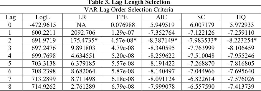
Table 3. Lag Length Selection VAR Lag Order Selection Criteria
Lag LogL LR FPE AIC SC HQ
0 -472.9615 NA 0.076988 5.949519 6.007179 5.972933 1 600.2211 2092.706 1.29e-07 -7.352764 -7.122126 -7.259110 2 691.9719 175.4735* 4.57e-08* -8.387149* -7.983533* -8.223254* 3 697.2476 9.891803 4.79e-08 -8.340595 -7.763999 -8.106459 4 699.7698 4.634551 5.20e-08 -8.259622 -7.510048 -7.955246 5 703.3138 6.379185 5.57e-08 -8.191422 -7.268870 -7.816805 6 708.2398 8.682064 5.87e-08 -8.140497 -7.044966 -7.695640 7 713.2899 8.711498 6.18e-08 -8.091124 -6.822614 -7.576026 8 714.9262 2.761289 6.79e-08 -7.999078 -6.557590 -7.413739
* indicates lag order selected by the criterion LR: sequential modified LR test statistic (each test at 5% level); FPE: Final prediction error AIC: Akaike information criterion; SC: Schwarz information criterion; HQ: Hannan-Quinn information criterion
831 5 percent level of significance once we used the real effective exchange rate and the nominal effective exchange rate as the dependent variables. It rejects the null hypothesis of no cointegration between the variables. This confirms the presence of two cointegrating vectors. This validates that there is a long run relationship between the variables over the period of 1971Q1-2012Q4 in the case of Nigeria.
Table 4. The Results of Bayer and Hanck Cointegration Analysis
Estimated Models EG-JOH EG-JOH-BO-BDM Cointegration
) ,
( t t
t f NER CPI
RER 17.888 33.169 Yes
) ,
( t t
t f RER CPI
NER 23.313 52.066 Yes
) ,
( t t
t f RER NER
CPI 2.653 6.462 No
Note: ** represents significant at 5 per cent level. Critical values at 1% level are 16.679 (EG-JOH) and 32.077 (EG-JOH-BO-BDM) respectively.
The long run results are reported in Table 5. We find that the nominal effective exchange rate affects the real effective exchange rate positively, and it is statistically significant at 1 percent level of significance. An increase of 1 percent in the nominal effective exchange rate is linked with 1.02 percent increase in the real effective exchange rate; all else is the same. The relationship of inflation (consumer price index) is positive and statistically significant at 1 percent. An increase of 0.773 percent in the prices of commodities in Nigeria will lead to increases the real effective exchange rate by 1 percent with other things constant. Simultaneously, the real effective exchange rate affects the nominal real effective exchange rate positively and is statistically significant at 1 percent level of significance. Meaning that, 1 percent increase in the real effective exchange rate will lead the nominal effective exchange rate to rise by 1 percent. The impact of inflation on the nominal exchange rate is negative and is statistically significant at 1 percent level of significance. We find that the nominal effective exchange rate leads the real effective exchange rate and vice versa in the case of Nigeria.
Table 5. Long Run and Short Run Analysis Long Run Analysis
Variables Dependent Variable =
t
RER
ln
Dependent Variable =ln
NER
t Coefficient T-statistics Coefficient T-statisticsConstant -2.7680* -13.8395 3.1917* 27.9172
t
NER
ln
1.0207* 38.9321 …. ….t
RER
ln
…. …. 0.8834* 38.9321t
CPI
ln
0.7728* 27.8784 -0.7832* -87.4805R2 0.9483 0.9938
Adj. R2 0.9477 0.9937
Short Run Analysis
Constant -0.0030 0.5646 0.0002 0.0438
t
NER
ln
1.0435* 46.263 …. ….1
ln
NER
t -0.3664* -4.7909 0.3211* 4.2660t
RER
ln
…. ….0.8900* 14.930
1
ln
RER
t 0.3073* 4.4156 -0.2610* -4.1108t
CPI
ln
0.5435* 5.5911 -0.4884* -4.31041
t
ECM
-0.0413** -2.3294 -0.0426* -3.0509R2 0.9344 0.9319
Adj. R2 0.9324 0.9298
832 The short-run results are also reported in Table 5 (lower segment). In this table, we find that the nominal effective exchange rate leads the real effective exchange rate at 1 percent level of significance. The impact of lagged difference term of the nominal exchange rate exerts a negative impact on the real exchange rate but becomes positive in the future period. The impact of inflation on the nominal effective exchange rate is positive and significant at 1 percent. The dependent variable is also positively affected by its own lag at 1 percent. It reveals that 1 percent increase in the real effective exchange rate in the previous period leads the real effective exchange rate in the current period by 0.30 percent. Table 5 shows the estimate of the lagged error term i.e.
ECM
t1 which is statistically significant at 1 percent with a negative sign. This indicates the speed of adjustment from the short run towards the long-run equilibrium path. Bannerjee et al. (1998) suggests that the“significance of lagged error term further validates the established long-run relationship between the variables”. We find that the coefficient ofECM
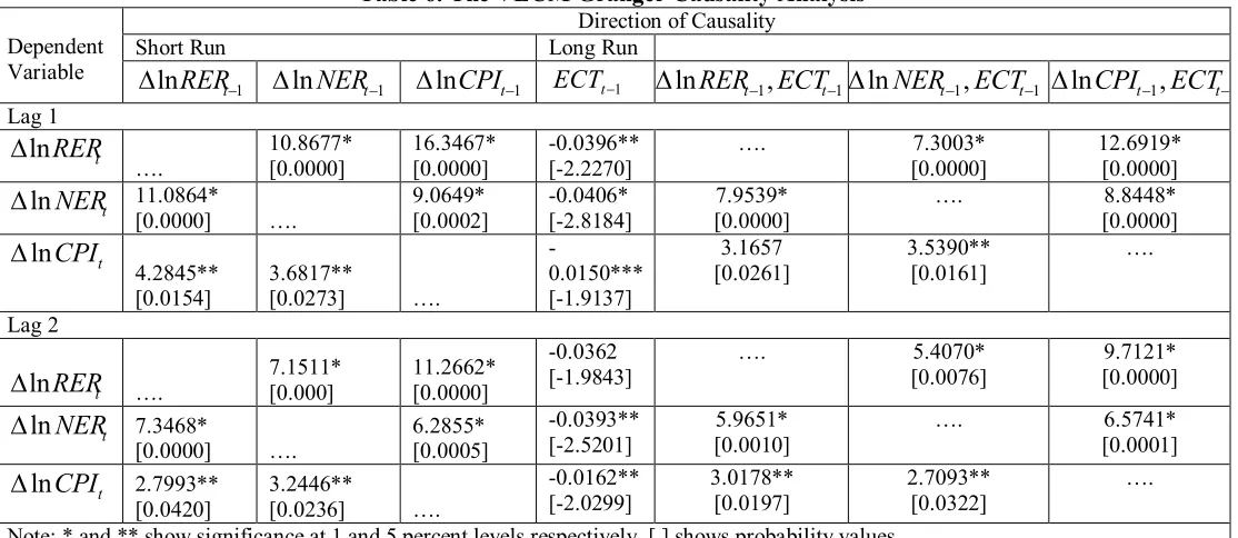
t1 is 0.0413 (0.0426), and it is significant at 1% level of significance. This means that the real effective exchange rate has corrected 4.13% (4.26) previous period disequilibrium. In other words, it will take almost 6 years (5 years and 8 months) to reach long-run equilibrium path of real effective exchange rate (nominal effective exchange rate) function in Nigeria.Table 6. The VECM Granger Causality Analysis
Dependent Variable
Direction of Causality
Short Run Long Run
1
ln
RER
t
ln
NER
t1
ln
CPI
t1 ECTt1
ln
RER
t1,
ECT
t1
ln
NER
t1,
ECT
t1
ln
CPI
t1,
ECT
t1 Lag 1 tRER
ln
…. 10.8677* [0.0000] 16.3467* [0.0000] -0.0396** [-2.2270]…. 7.3003*
[0.0000] 12.6919* [0.0000] t
NER
ln
11.0864*[0.0000] ….
9.0649* [0.0002] -0.0406* [-2.8184] 7.9539* [0.0000]
…. 8.8448*
[0.0000] t
CPI
ln
4.2845** [0.0154] 3.6817**[0.0273] ….
-0.0150*** [-1.9137] 3.1657 [0.0261] 3.5390** [0.0161] …. Lag 2 t
RER
ln
…. 7.1511* [0.000] 11.2662* [0.0000]-0.0362 [-1.9843]
…. 5.4070*
[0.0076] 9.7121* [0.0000] t
NER
ln
7.3468*[0.0000] ….
6.2855* [0.0005] -0.0393** [-2.5201] 5.9651* [0.0010]
…. 6.5741*
[0.0001] t
CPI
ln
2.7993** [0.0420] 3.2446**[0.0236] ….
-0.0162** [-2.0299] 3.0178** [0.0197] 2.7093** [0.0322] ….
Note: * and ** show significance at 1 and 5 percent levels respectively. [ ] shows probability values.
833 6. Conclusion, Policy Implications and Recommendations
Nigeria is a country that has been depending on oil as its key export commodity for decades and this situation has led to the neglect of many vital economic resources, thereby breeding a cancerous mono economic dependence situation in the country for decades. This situation in turn creates massive unemployment and an alarming paucity of external accruals to finance the lingering poverty of the country (all things being equal). Similarly, several economic indexes and researchers have been pointing out delusive and inconclusive growth attainment of the country which has not impacted positively on the populace. It is along the line of this development that this study reinvestigated the relationship between the nominal effective exchange rate and the real effective exchange rate. In a bid to make a unique contribution in this study, we further incorporate inflation as an additional determinant of nominal and real effective exchange rates and utilized time series data from the periods of 1971QI to 2012QVI. The main objective is to assess if there are possible competitive opportunities for the country to move progressively in international trade in terms of tradable goods with minimal hurdles, thus exploring the fitness of the Marshall-Lerner assumption (M-L) to the case of Nigeria. In doing so, we applied traditional and structural break unit root tests to the series, while the presence of cointegration between the variables was explored using the Bayer-Hanck cointegration approach. In addition to this, the direction of the causal relationship between the nominal and the real effective exchange rates is investigated by applying the VECM Granger causality test.
Interestingly, the findings of the study suggest the presence of cointegration between the variables, meaning that nominal effective exchange rate leads to the real effective exchange rate. While the most impressive and surprising discovery is that moderate inflation eats up the unfavorable impacts of nominal devaluation in the case of Nigeria. The results from the causality analysis, on the other hand, confirmed the existence of effective feedback between the real and the nominal effective exchange rates, and between the nominal effective exchange rate and inflation and between inflation and the real effective exchange rate.
Overall the findings of this study suggest that a moderate depreciation of the Nigerian local currency may, in fact, have stabilizing influence on the balance of payments through the current account, without the need for imposing high-interest rates. As a result of this, we hold the opinion that a less contractionary monetary policy by the Central Bank of Nigeria could, in fact, be combined with an appropriate exchange rate policy to achieve more effectively the objectives of devaluation in Nigeria. This would be a better option than the current high-interest rate policy being pursued by the Central Bank, which in the long run ends up in stifling economic growth. Finally, we believe that the findings of this study will help in formulating comprehensive trade policy in Nigeria including the use of efficient and effective devaluationary strategies for enhancing international trade. In our concluding remark, we argue that, in order to achieve the benefits of the Marshall-Larner assumptions in Nigeria, we propose considerable need for massive infrastructural provision (particularly electricity) in the country. This should in turn encourage manufacturers to engage in production quality; product differentiation, innovation and product specialization. Additionally, the domestic industries should be liberalized and strategized towards international competitive operation by enhancing their capacity to expand commensurate with the new demand. The proposed findings to our believe will help in reducing the J-curve effect as found in the case of Kenya by Guglielmo et al. (2012)
References
Adam, C.S, B.O. Maturo, N.S. Ndung’u. O’Connell S.A. (2010).Building a Kenyan Monetary Policy Regime for the Twenty-first Century in C.S. Adam, P. Collier and N.S. Ndung’u (eds) Kenya: Policies for Prosperity Oxford University Press.
Bahmani,-Oskooee, M. (1998). Are Devaluations Contractionary in LDCs? Journal of Economic Development, 23(1), 131-38.
Bahmani-Oskooee, M., Mirzai, I. (2000). Real and Nominal Effective Exchange Rates for Developing Economies: 1973-1997. Applied Economics, Issue-4, 411-428.
Bahmani-Oskooee, M., Miteza, I. (2002).Do Nominal Devaluations Lead to Real Devaluations in LDCs?Economics Letters, 74, 385–91.
Bahmani-Oskooee, M, Kutan, A.M. (2008).The J-curve in the emerging economies of Eastern Europe.
834 Bannerjee, A., Dolado, J., Mestre, R. (1998).Error correction mechanism tests for co-integration in
single equation framework, Journal of Time Series Analysis, 19, 3, 267-283.
Bayer, C., Hanck, C. (2012).Combining non-cointegration tests, Journal of Time Series Analysis. DOI: 10.1111/j.1467-9892.2012.814.x
Boswijk, H.P. (1994).Testing for an unstable root in conditional and unconditional error correction models, Journal of Econometrics, 63(1), 37–60.
Bruno, M. (1978). Exchange Rates, Import Costs, and Wage-Price Dynamics, Journal of Political Economy, 86, 379–403.
Cooper, N. (1971).Currency devaluation in developing countries. In: Ranis G (ed) Government and economic development. Yale University Press, New Heaven, pp 26–42.
Connolly, M., Taylor, D. (1976).Adjustment to Devaluation with Money and Non-Traded goods,
Journal of International Economics, 6: 289–98.
Connolly, M., Taylor, D. (1979.Exchange Rate Changes and Neutralization: A Test of the Monetary Approach Applied to Developed and Developing Countries, Economica, 46, 281–94.
CopelmanM, Werner AM (1996) The monetary transmission mechanism in Mexico. Working Paper, Federal Reserve Board.
Dickey, D., Fuller, W.A. (1979). Distribution of the Estimates for Autoregressive Time Series with Unit Root, Journal of the American Statistical Association, 74, 427-31.
Edwards, S (1986). Are devaluations contractionary? Rev Econ Stat, 68, 501–508.
Edwards, S. (1988).Real and Monetary Determinants of Real Exchange Behavior: Theory and Evidence from Developing Countries. Journal of Development Economics, 29, 311 – 341. Edwards, S. (1994). Real and Monetary Determinants of Real Exchange Rate Behavior: Theory and
Evidence from Developing Countries. In J. Williamson (eds.). Estimating Equilibrium Exchange Rates. Washington, D.C.: IIE. (Chapter 4).
Elliot, G., Rothenberg, T.J., Stock, J.H. (1996), Efficient Tests for an Autoregressive Unit Root,
Econometrica, 64, 813-36.
Engle, R.F., Granger, C. (1987).Cointegration and error correction representation: Estimation and testing. Econometrica, 55(2), 251–276.
Fisher, R. (1932), Statistical methods for research workers. London: Oliver and Boyd.
Granger, C.W.J. (1969). Investigating causal relations by econometric models and cross-spectral methods. Econometrica 37, 424–438.
Guglielmo, C. Gil-Alana, M. Luis A.., Robert, M., (2012) Testing the Marshall-Lerner condition in Kenya, Discussion Papers, German Institute for Economic Research, DIW Berlin, No. 1247 Johansen, S. (1995), A statistical analysis of cointegration for I(2) variables. Econometric Theory,
11(2), 25-59.
Kamin, S.B., Rogers, J.H. (2000)Output and real exchange rate in developing countries: an application to Mexico. J Dev Econ 61:85–109.
Kent, C, Naja, R, (1998).Effective Real Exchange Rates and Irrelevant Nominal Exchange Rate Regimes, Research Discussion paper n. 9811.
Krugman, P. Taylor, L. (1978).Contractionary effects of devaluation. Journal of International Economics 8, 445–456
Kwiatkowski, D., Phillips, P.C.B. Schmidt, P., Shin, Y. (1992). Testing the null hypothesis of stationarity against the alternative of a unit root. Journal of Econometrics, 54, 159-178.
Lizondo, J.S, Monteil, P.J. (1989).Contractionary devaluation in developing countries. International Monetary Fund Staff papers 36, 182–227
Mcteer, B. (2008) The Impacts of Foreign Trade on the Economy. Business day, The New York Times: http://economix.blogs.nytimes.com/2008/12/10/the-impact-of-foreign-trade-on-the-economy/?_r=0
Mejia-Reyesab, P., Osboma, D.R, Sensier, M. (2010).Modeling real exchange rate effects on output performance in Latin America. Applied Economics, 42, 2491–2503.
Miteza, I. (2006).Devaluation and output in five transition economies: a panel cointegration approach of Poland, Hungary, Czech Republic, Slovakia and Romania, 1993–2000. Applied Econometrics International Development, 6(1), 69–78.
835 Oyejidi, T.A. Adewuyi, A.O. (2011).Enhancing linkages of oil and gas industry in the Nigerian economy. Trade Policy Research and Training Programme (TPRTP), MMCP Discussion Paper No. 8, Department of Economics, University of Ibadan.
Ozurumba, B.A., Chigbu, E.E. (2013).Non-Oil Export Financing and Nigeria’s Economic Growth.
Interdisciplinary Journal of Contemporary Research in Business, 4(10), 133-148.
Pesavento, E. (2004).Analytical evaluation of the power of tests for the absence of cointegration,
Journal of Econometrics, 122(2), 349–84.
Phillips, P.C.B., Perron, P. (1988).Testing for a unit root in time series regression, Biometrika, 75, 335-346.
Rafindadi, A.A., Yusof, Z. (2014). Do the dynamics of financial development spur economic growth in Nigeria’s contemporal economic growth struggle? Facts beyond the figures, Journal of Quality and Quantity, DOI: 10.1007/s11135-014-9991-0
Rafindadi, A.A., Yusof, Z.(2013) A Startling New Empirical Finding on the Nexus Between Financial Development and Economic Growth in Kenya. World Applied. Sciences. Journal, 28, 147-161,
Ratha, A, (2010). Does devaluation work for India? Economic Bulletin, 30, 247–264.
Sheeley, C.A. (1986) Unanticipated inflation, devaluation and output in Latin America. World Development, 14, 65–71.
Stern, D. (1973) in Brooks, T. J. (1999). Currency depreciation and the trade balance: an elasticity approach and test of the Marshall-Lerner condition for bilateral trade between the USA and the g-7. Unpublished PhD thesis, The University of Wisconsin-Milwaukee.
Ugbede, O., Lizam, M., Kaseri, A., Robert, M.S. (2013) Does oil and non-oil balance of trade impact similarly on Malaysia and Nigeria GDP? International conference on Economic, Finance and Management Outlook (ICFEMO) 6-8th December, 2013 Pearl International Hotel, Kuala Lumpur.
Vaubel, R. (1976), “Real Exchange Rate Changes in the European Community: The Empirical Evidence and its Implications for European Currency Unification”.Weltwirtschaftliches Archive, 112, 429–70.
Yesufu, T.M. (1996). The Nigerian Economy: Growth without Development. Benin City; University of Benin Press. pp. 1-400