Ethnic Violence Across Space
Hannes Mueller Dominic Rohner David Sch¨onholzer*
June 3, 2020
Abstract
Ethnic violence requires spatial proximity between ethnic groups, but the role of distance between groups for conflict remains understudied. We develop a structural model of spatial vio-lence in which ethnic groups recruit fighters strategically across space to maximize their impact. Spatial decay of violence determines the equilibrium placement of fighters and implies specific spatial patterns of conflict. We then estimate the structural parameters of the model using fine-grained data on ethnic groups and violence from 24 ethnically divided countries. We find that in more than half of these, spatial decay is substantial: half of all ethnic violence dissipates after 350km. Consequently, violence is higher near ethnic borders, although a substantial share of violence originates from distant locations. Using the estimated parameters of the model, we also find that ethnic conflict is strongly asymmetric, especially in states with higher state capac-ity. Counterfactual estimates suggest that setting up barriers can reduce violence but pacifying groups with more grievances is often more effective.
Keywords: Conflict, Ethnic Violence, Spatial Data, Distance Costs, Polarization, Fraction-alizaton, Segregation, Insurgency.
JEL Classification: D74, K42, Z10.
*Mueller: Institut d’Analisi Economica (CSIC), Barcelona GSE and CEPR (email: [email protected]).
Rohner: Department of Economics, University of Lausanne and CEPR (email: [email protected]). Sch¨onholzer: Institute for International Economic Studies, Stockholm University (email: [email protected]).
Acknowl-edgements: We thank Nezih Guner and three anonymous referees for very helpful suggestions. Further, we are grateful to Quentin Gallea, Yihuan Hu, Dong Ook Eun, Augustin Tapsoba and Nghia-Piotr Trong Le for excellent research assistance, and to Joan Maria Esteban, Mathias Thoenig, and Debraj Ray for useful comments. We also
thank seminar participants at Institut d’Analisi Economica (CSIC), UC Berkeley, NYU Abu Dhabi, and CEMFI Madrid, and participants to the IEA World Congress, Barcelona GSE Summer Forum, EEA annual congress in Geneva, ENCoRe Bonn, ”Social Interactions, Norms and Development” conference in Moscow, Swiss Development
Network workshop in Fribourg, and the ”Conflict Prediction for Prevention” conference in Barcelona. All errors are of course ours. Hannes Mueller acknowledges financial support from Grant number ECO2015-66883-P, the Ramon y Cajal programme and the Severo Ochoa Programme and Dominic Rohner is grateful for financial support from the
1
Introduction
For several decades, the role of ethnic diversity in conflict has been a major focal point for
aca-demics, NGOs, politicians and journalists alike. Strikingly, however, the emphasis has been almost
exclusively on nationwide ethnic population composition, ignoring the location of groups. This
omission weighs heavily, as ethnic demography on its own can only explain a mere tenth of violence
eruptions.1 Indeed, the heterogeneity of outcomes even for the most ethnically polarized countries
is impressive (see Montalvo and Reynal-Querol 2005 for ethnic polarization definition and data):
For every high-polarization country with recent conflict (say, Guatemala, Afghanistan, Northern
Ireland, Sri Lanka) there are others that are equally ethnically polarized but have been peaceful
for decades or even centuries (Jordan, Mauritius, Switzerland, Malaysia).
In order to capture this heterogeneity in the fate of ethnically diverse countries, we move beyond
ethnic population shares by addingspace to the equation. The motivating rationale for the focus on
spatial interaction is that interactions between people are typically easier, and hence more intense
and frequent, when they are geographically close. This decay of interaction with increasing distance
has been found in various fields of economics. For example, trade economists refer to “iceberg trade
costs” increasing in distance and use “gravity models of trade” to account for the fact that trade
between more distant places is more costly, and drawing on this spatial decay has proven fruitful
to explain the distribution of economic activity across space (see e.g. Fajgelbaum et al. 2017 and
Donaldson 2018).2
To integrate space into the study of ethnic conflict, we build a novel game-theoretic model of
ethnic interactions across space and estimate the structural parameters of the model. In our setting,
each ethnic group strategically recruits fighters across heterogeneous locations to maximize their
spoils of conflict, taking into account the spatial composition of opposing groups in the vicinity
and local support in the homelands. This leads to specific predictions how the interaction of
spatial distance and population distributions matters for conflict intensity. We then estimate the
parameters of our structural model for 24 countries with substantial ethnic conflict (drawing on
the classification by Kalyvas and Balcells 2010, as discussed in detail below). For each country, we
estimate the extent to which spatial distance is a key feature of strategic conflict interactions, as
well as a series of further parameters related to fighting motivation, reliance on local support and
the spatial origins of attacks. It turns out that for 13 out of 24 countries space is a key element of
conflict interaction and for the median spatial decay we find that attack effectiveness is reduced by
half over a distance of 350 km.
1
See e.g. column 1 in Table 1 of Esteban et al. (2012) where nationwide ethnic diversity measures and total population together account for 13 percent of variation in conflict onsets.
2
Our setting also allows us to estimate the shares of violence crossing district borders, the
group-level stakes of conflict and the relative aggressiveness of a given group (i.e. the difference between
the attacks perpetuated versus suffered). These parameters and measures endow our framework
with substantial additional explanatory power relative to widely used country-level diversity
mea-sures such as ethnic polarization. We also demonstrate that by separating targets and perpetrators
of violence our model provide several meaningful statistics like the share of violence inflicted across
locations, the aggressiveness of groups or the asymmetry of the ethnic conflict. To interpret our
results, we also relate our estimated parameters to topographic, geological and demographic
covari-ates. Finally, the estimates of our structural model allow us to perform counterfactual estimations,
highlighting the country-specific violence potential linked to changing spatial decay.
Our findings provide several new insights into the nature of ethnic conflict. First, we document
in simple reduced-form regressions that conflict is more intense in locations near ethnic boundaries:
if a location is 10% closer to an ethnic boundary, it suffers 1.3% more conflict casualties than
comparable locations. Second, this reduced-form finding masks substantial heterogeneity in the
extent of spatial decay in our structural model: some countries show little evidence of distance
decay, while for others almost all violence may dissipate even after 100km. Third, as a result of
this decay of violence across space, the location of strategically placed fighters and the resulting
violence in a location may depend on the spatial composition of ethnic groups across the entire
country. Thus, conflict in a given location may originate almost entirely from other places: across
the 24 countries in our sample, we associate more than three quarters of ethnic violence in a district
to the ethnic composition of surrounding districts as opposed to its own. Fourth, the extent to
which violence emanates from outside a location is strongly driven by group-specific motivations
to engage in violence with others. We find that this engagement exhibits substantial asymmetry:
some groups instigate almost all ethnic violence in a country, while others seem to be mostly on
the receiving end of aggression.
Two caveats apply to our argument. First, we study how geographical proximity affects the
risk of attacks in ongoing conflicts. This focus makes perfect sense in the short-run when fighting
is acute. However, in the long-run, positive interactions between ethnic or religious groups could
build trust between them and the actual motives for attacks may be reduced (see Rohner et al.
(2013b). Hence, while bigger geographical distances can indeed reduce the number of attacks
during a conflict (as emphasized by the current paper), in post-conflict reconstruction ”building
bridges” and reducing inter-group distance may be important policies to re-enforce peace. This
subtle point has important policy implications: While physically separating groups (e.g. through
the construction of barriers) may indeed be justifiable while fighting is still virulent, it may be
to measure the support bases of the groups engaged in conflict. This is important, as these bases
produce the support needed for violence becoming visible elsewhere. In this study we rely on the
location of ethnic homelands to capture support bases and show that, even with this crude measure,
our model is able to provide several new insights. However, our work should still be seen as only a
first step in bringing the notion of space and the separation of attackers and targets to the empirical
study of conflict.
Our paper is linked to several strands of the literature. In particular, it is related to the
theoretical literature on ethnic and religious conflict (e.g. Horowitz 2000; Varshney 2001; Esteban
and Ray 2008; Rohner 2011; Caselli and Coleman 2013; Rohner et al. 2013b), and the empirical
studies linking ethnic diversity to civil war at the country-year level (see Fearon and Laitin 2003;
Collier and Hoeffler 2004; Montalvo and Reynal-Querol 2005; Cederman and Girardin 2007; Collier
et al. 2009; Esteban et al. 2012; Michalopoulos and Papaioannou 2016). These articles generally
find that ethnic heterogeneity (and in particular ethnic polarization) increases the risk of conflict,
but – contrary to our current contribution – they do not study the spatial patterns of ethnic
violence.3 Our main contribution here is to show that, holding the overall size of different ethnic groups (i.e. ethnic polarization or fractionalization measures) fixed, overall levels of violence will
differ dramatically depending on how the populations are distributed in space. In this regard our
work directly relates to studies on the impact of segregation, with some scholars finding that it
increases the risk of ethnic conflict (Medrano, 1994; Olzak et al., 1996), while others argue that
partition could be a solution to ethnic conflict (Horowitz, 2000).4
In terms of further related literatures, in recent years there has also been an increasing number
of papers studying violence at a disaggregate, local level (e.g. Harari and Ferrara 2018; Rohner et al.
2013a; Dube and Vargas 2013; Berman et al. 2017; K¨onig et al. 2017; Huber and Mayoral 2019).
Also the micro-level literature on insurgency and counter-insurgency is relevant (see Kalyvas 2006;
Lyall 2010; Bhavnani et al. 2011; Kocher et al. 2011; Berman et al. 2011). Some of these studies
stress the importance of territorial control for understanding how violence evolves in civil war. This
provides a key stepping stone for our model as it provides the idea of bases of support which come
with territorial control over population or resources. Importantly, however, none of these studies
provide a formal model of conflict in which the location of attackers and targets differs. As this
literature moves into more and more disaggregated data, the confounding of motivation, origin and
destination of attacks will become problematic, as the drivers of conflict like economic deprivation,
ideology, ethnic hatred or the presence of natural resources may be increasingly spatially separate
from where attacks are observed. Our model is able to account for this, by allowing attackers to
3The results in Spolaore and Wacziarg (2016) suggest that this may not hold for international wars where
geneti-cally similar populations are engaged more in conflict.
4
operate or draw support from other locations than the targets of violence.
Maybe closest to our contribution is the literature focusing on spatial patterns of violence. There
is a small literature in political science studying –inspired by the epidemiological literature on the
spread of diseases– diffusion and clustering patterns of violence over space and time (Townsley
et al., 2008; Schutte and Weidmann, 2011). Further, Novta (2016) builds a simulation-based model
of how conflict spreads dynamically in space. She models the armed groups in 109 municipalities
as separate players who can only attack in their home village while the focus of our framework lies
precisely in providing a model of attacks across regions.5 Bhavnani et al. (2014) link segregation to urban conflict, using a simulated agent-based model, calibrated for Jerusalem. Finally, the empirical
contribution of Balcells et al. (2016) studies post-conflict sectarian clashes in Northern Ireland from
2005-2012. A main difference between our current paper and the existing work on spatial violence
patterns is that –contrary to the existing literature– our empirical analysis estimates a structural
model of conflict in space. We are able to derive such a model by assuming that conflict is motivated
by aggregate factors - exactly as the ”macro” contest literature does (see Konrad 2009). In this way
we build a link from the newer studies using micro data to the classic theoretical models studying
the intensity of conflict at the country level.
The predictive power of our framework is useful when it comes to forecasting the impact of
conflict on economic outcomes. Besley and Mueller (2012) show for Northern Ireland that compared
to peaceful areas, housing in the most violent areas sold for between 2 and 17 percent less
-depending on the level of violence, and Mueller (2016) shows that changes in the distribution of
violence within a country can have a substantial impact on aggregate growth. Thus, predicting
well the location of attacks does not only help in forecasting local economic outcomes, but also
countrywide performance.
The paper is organized as follows: Section 2 sets up a simple model of spatial interaction. In
Section 3 we introduce the data used and display reduced-form stylized facts. Next, while Section
4 is devoted to a detailed account of our structural estimation, in Section 5 we carry out the
econometric analysis and present the main results and robustness checks. Section 6 provides a
counter-factual policy analysis and Section 7 concludes. Appendices provide further details and
results.
2
Model
We begin the model exposition of how space matters for armed conflict by setting up an environment
with multiple ethnic groups spread across many districts. Groups may endogenously recruit fighters
from their own ethnic groups at some cost, who can conduct attacks on other groups in their district
as well as all other districts depending on how difficult it is for them to project violence across space.
After laying out the foundations of the model, we derive the equilibrium placement of fighters,
which gives us an expression for predicted violence in a district as a function of the spatial
distri-bution of groups across all districts, the extent of spatial decay of violence, local recruitment cost,
and group-specific features driving the level of their engagement in the conflict. Once we
character-ize the equilibrium, we derive various novel country-level and group-level indices capturing salient
features of spatial violence and shedding new light on the nature of ethnic conflict. Finally, we
discuss the assumptions underlying the model in the context of existing models of conflict.
2.1 Setup
We model conflict between groups g, k = 1, ..., G which are residing in regions i, j = 1, ..., J. The
population of group g in region i is given by Nig. We denote group population aggregates as
Ng =PJi=1Nig. Our model integrates two ideas. First, attacks happen across space. In particular,
attacks by fighters of groupgin regionion groupkin regionjare governed by a distance parameter
wij. Attacks on this dyad are then given by
Aijgk =Fig·wij ·Njk,
which makes clear that our model has a spatial dimension. Theoretically, the distance weightswij
could take many forms. In the empirical model we will assume a simple functional form
wij = exp (−κ·distance(i, j))
so that for κ >0 we will see fewer attacks between locations that are further apart.
The second key assumption is that the recruitment of fighters Fig is endogenously determined
by the struggle of all groups at the macro level. Specifically, we assume that the expected benefits
of conflict to group g are given by a conflict prizeRg times the probability of winning the contest
given by
Ag PG
k=1Ak
Rg,
where Ag is the total number of attacksAijgk of groupg across all districts and opposing groups.
This is the standard contest success function and is widely used in the conflict literature (see the
literature survey in Konrad 2009). This implies that we are able to describe aggregate violence as a
allows us to estimate the model despite the fact that the recruitment of fighters is endogenous and
determined locally.6
Groupg recruits local fighters, Fig in regions i= 1, ..., J, to maximize the objective function
πg=
AgRg PG
k=1Ak
−1
2
J X
i=1
Fig2 Nigµ.
The first term are the expected benefits of attacks, while the second term captures the fact that
recruiting fighters is costly. We make this specific cost function assumption only for simplicity.
Two aspects are critical: First, we model the cost function as convex in the number of fighters to
ensure an equilibrium.7 Typically, salary costs of fighters should be thought of as convex, as the first few hirings will be cheap given that it will be feasible to target exclusively individuals with low
wages in the regular economy (and hence low opportunity costs of fighting) and/or with low moral
costs of killing. When extending the pool of fighters in a region, the group also needs to recruit
individuals with better outside options and higher moral costs who will require higher monetary
compensation.
The second key aspect of the payoff function is that recruitment costs of fighters are a function
of the local population. More specifically, the larger the population of locals of a given group
in a given region, the cheaper the hiring costs, i.e. µ ≥ 0. This assumption makes sense in a
context where fighters face lower risks of identification and being arrested and can benefit from
local support through information and safehouses. This assumption finds considerable backing in
military guides like the US counter-insurgency manual (Army and Corps, 2006) and the existing
literature in political science (Kalyvas, 2006) which both stress the role of local informants in civil
wars. This means that even professional armies will require the support of local population when
fighting in asymmetric wars. We discuss these assumptions in greater detail in Section 2.6.
To close the model we will use matrix notation as this simplifies the description of optimal
fighting effort. Denote the group-specific vector of district populations as a J ×1 vector Ng =
(N1g, ..., NJ g)0 and theJ×J spatial weights matrixW = (W1, ...,WJ) withWi = (wi1, ..., wiJ)0.
Total attacks projected by groupg from region iare then
Aig =Fig J X
j=1
wijNj,−g =FigWi0N−g (1)
6
We assume throughout thatRg >0, which implies that all groups in a country are engaged in conflict. This
ensures the existence of an interior solution in our model. In the empirical implementation we will also assume that
Rg >0, but will allow the group-specific value ofRg to be arbitrarily close to zero to capture groups that inflict very
little violence.
7
where Nj,−g = Pk=6 gNjk denotes the population of all groups that are not g at location j and N−g = Pk6=gNk is the corresponding vector of total population in all groups that are not g in
locationsj = 1, ..., J. Similarly, instead of examining attacks by groupgemanating fromi, we can
write violence against groupg in regionifrom all other regions as
Vig =Nig J X
j=1
wijFj,−g =NigWi0F−g, (2)
where F−g is a J ×1 vector with elements Fj,−g = Pk6=gFjk. This expression shows that the
amount of violence against g in i is the product of its local population size Nig and the spatial
projection of all opposing fighters onto region igiven byW0iF−g.
2.2 Equilibrium Spatial Violence
The equilibrium solution to this model is surprisingly simple. Equilibrium fighters of group g in
regioniare given by
Fig∗ =αgNigµWi0N−g (3)
where αg = RgA−g
(PG k=1Ak)
2 only varies at the group level. In other words, we can express the fighting
effort at each location simply through the interaction of aggregate, strategic incentives (αg) with
the local interaction of population in space (NigµW0iN−g). Empirically it will be important thatαg
is merely a scaling factor that only varies across groups but not locations - this will allow us to
identify the parameters of the model through local variation in population and violence. Inserting
(3) into (2) and aggregating across all groups, we get all equilibrium attacks into regioni:
Vi∗=
G X
g=1
NigW0i X
k6=g
αkdiag Nµk
WN−k, (4)
where diag(·) turns the vector Nµk into a J ×J diagonal matrix with elements Njkµ on the diagonal and zeros on the off-diagonals. Existence and uniqueness are shown below in Appendix
A.1. The expression in equation (4) fully captures the mechanics of conflict posited in our model:
the last term in equation (4), the J ×1 vector WN−k, captures the incentives for group k to
recruit fighters in each district, depending how easy it is to reach targets. If many opposing groups
are clustered in a location, it is more appealing to place fighters there. The middle term, the
1×J vectorW0iP
k6=gαkdiag Nµk
, captures the average distance to the support bases of fighters
to conduct violence in location i. This depends on the engagement of groups in the conflict, αk,
location i. Finally, the third expression, the scalar PG
g=1Nig, is the sum of all potential victims
across all groups ini. The product of these three terms is the amount of violence inipredicted by
the model.
Distance enters in this formula through the weights of the weighting matricesWi andW. Low
values in Wi shield locationi from outside attacks as fighters from other locations cannot attack
it easily. The weighting matrix W appears also at the end of the equation because it determines how many fighters are recruited in other locations j.
2.3 Illustration
Despite its simplicity, the model generates complex spatial interactions represented in equations
(1) and (2). To illustrate these interactions we show a simple example with two groups at three
locations in Figure 1. The locations are called 1, 2 and 3 and the groups are called R (red) and B
(blue).
In the top panel A, we show the incoming attacks by group B into location 1 on group R. This
is the kind of data that a typical violence dataset would provide - the violence suffered by targets
at a location. Group R at location 1 is attacked by blue fighters stationed in the same location,
F1,B. These fighters have N1,R targets at location 1 and a distance weight w1,1 so that violence
from blue fighters at location 1 is given by F1,Bw1,1N1,R. Blue fighters at locations 2 and 3 also
attack the red population at location 1, only now the distance weights are given by w1,2 and w1,3.
If distance plays a role we would expect thatw1,1> w1,2, w1,3 so that the blue fighters at location
1 are more effective in attacking red population at location 1.
A key advantage of the model is, however, that we can use the estimated parameters to provide
estimates of outgoing violence as well. In the bottom panel B, we show the outgoing attacks by
red fighters at location 1 into other regions. With the estimated parameters of the model this
violence can be easily calculated. These fighters have N1,B targets at location 1 and a distance
weight w1,1 so that violence from red fighters at location 1 is given by F1,Rw1,1N1,B. Panel B also
illustrates nicely that the recruitment of fighters at a location will be a function not only of the
potential target population at that location but also of targets nearby. In the example, recruitment
of fighters at location 1 is partly driven by the blue population at locations 2 and 3. This feature
makes the spatial dynamics of the model non-trivial as the incoming attacks in panel A will be a
function of the respective neighbourhoods of location 2 and 3, given that fighters at those locations
are recruited with targets in mind.
With higher spatial decay, i.e. quickly fallingwij with longer distance, recruitment at a location
will mostly be driven by the population that lives in that region. In the example, this would imply
two groups do not mix then violence is reduced. The opposite case is where there is very little
spatial decay. In the example this would imply, for example, that the number of red fighters
is only a function of the population from which the fighters can be recruited from, i.e. the red
population. The recruitment of red fighters would then be motivated by total blue population
(N1,B +N2,B +N3,B) and, assuming µ > 0, be stronger in location 2 as it has a larger red
population.
2.4 External Violence, Aggressive Groups and Asymmetry
The model of spatial interactions offers the opportunity to understand conflict data in a new light
by separating perpetrators from targets. We use the model to calculate three statistics, which have
an immediate interpretation and can help understand the conflict dynamics of a country.
The first summary statistic that we can calculate is the share of all violence at a given location
that travelled from outside that location. This statistic separates the violence coming from fighters
at the same location from the violence originating from other locations. To calculate the share we
first calculate the total sum of violence at locationias:
Vtotal∗ =
J X
i=1
Vi∗ =
G X
g=1
X
k6=g
N0gWF∗k,
whereF∗k is the vector of equilibrium fighters for group kgiven by:
F∗k=αkdiag Nµk
WN−k.
We can contrast this with the violence emanating only from within a given region. In the matrix
notation this can be derived with a simple change in the spatial weights, by only letting these
fighters attack who are in the same region. This is done by changing the attack weighting matrix
toW= diag (w11, ..., wJ J). We call this local violence:
Vlocal∗ =
G X
g=1
X
k6=g
N0gdiag (w11, ..., wJ J)F∗k.
This implies that we can write the share of violence from outside as:
vexternal=
Vtotal∗ −Vlocal∗ Vtotal∗ =
PG g=1
P
k6=gN0gWFf ∗k PG
g=1
P
k6=gN0gWF∗k
, (5)
share of violence coming from outside locations. We regard vexternal as an important statistic to
capture the extent of violence being “mis-attributed” to a target location despite the fact that
it originated from fighters at other locations. For studies using disaggregated data to assess the
drivers of conflict, expression 5 is an important object to study.
Incoming and outgoing violence are also useful to understand how “aggressive” groups are by
comparing the number of casualties that they suffer to the attacks that they inflict. Note that the
sum of attacks inflicted by group gacross all districts is simply
A∗g,total≡
J X
i=1
A∗ig =F0∗gWN−g,
while the sum of violence against groupg across all districts
Vg,∗total ≡
J X
i=1
Vig∗ =N0gWF∗−g.
Hence, at the country level we can write:
Vtotal∗ =A∗total =
G X
g=1
X
k6=g
N0gWF∗−g
and at the group level we calculate an index ag,aggressive given by
ag,aggressive=
A∗g,total−Vg,∗total
Vtotal∗ , (6)
which is positive if a group is inflicting more casualties than it is suffering and negative if it is
suffering more casualties. The index ranges from −1 to 1, where −1 captures that a group is
suffering all violence in the country and 1 that it is generating all violence in the country. If groups
inflict as many casualties as they suffer, ag,aggressive will be close to 0.
From this index, we can easily calculate an index of asymmetry of violence at the country level:
aasymmetric=
1 G
G X
g=1
|ag,aggressive|=
1 G G X g=1 PJ i=1 A ∗
ig−Vig∗ PG k=1 PJ i=1Vik∗
, (7)
which captures the average, absolute aggressiveness score. Thus, if all groups inflict the same
number of casualties as they suffer, then aasymmetric = 0. In contrast, if some groups conduct all
2.5 Ethnic Interaction versus Nationalized Violence
As we are interested in analyzing the extent of spatial interactions, we will focus on the case of
µ > 0 for most parts of the paper. This assumption implies that fighters cannot be recruited ad
hoc in regions without local support, where local support should be seen as a broad concept which
includes situations where the local population will provide information to stationed troops.
The central empirical question is then how much spatial decay there is.8 If spatial weights are decreasing, our model generates violence patterns where violence clusters in ethnically mixed,
densely populated areas. This is because average distance between targets and fighters will be
smallest (wij will be highest) where ethnic groups mix, leading to more intense recruiting of fighters
in equilibrium. We call such a type of conflict ethnic interaction. The illustration in Section 2.3
presents a simple example of such a case.
If µ >0 but all weights are the same (wij = wi0j0 for all i, j, i0, j0) then the distance between
fighters and targets is not important and the attacks on Nig are simply a function of conflict
motivationRg and the total population Nbut not how concentrated population is in space. If we
normalize wij = 1 we can re-write the optimal recruitment of fighters
Fig∗ =αgNigµ
X
j X
k6=g
Njk
(8)
so that the local recruitment of fighters at locationiis now only a function of the total number of
targets in the country, the motivationαg and the ability to recruit locallyNigµ. Military technology
will obviously play a role here as the use of mobile units, for example, would mean that it is better
to build strong military bases and start attacks from there. Violence in locationiis then given by
Vi∗ =
G X g=1 Nig X
k6=g X
i
Fik∗
(9)
which is simply the number of all fighters in all other regions attacking the population at locationi.
This will generate violence patterns in which violence follows target population without the spatial
patterns of ethnic interaction violence. We call such violence patternsnationalized violence.
2.6 Discussion of Model Assumptions Relative to Alternative Settings
Key assumptions of the modeling strategy concern the payoff functions. In particular, we assume
that the groups’ winning chances depend on the number of successful attacks rather than e.g. on
8
the number of fighters they field. This reflects the view that realized attacks matter more than
potential ones, and is also in line with the available micro-level data that contains information on
fighting events but not on troop strength (see Section 3 below). Further, in our model recruitment
and fighting efforts of a groupg in a regionionly depend on i) the aggregate nationwide strategic
interaction and ii) the demographic spatial distribution of the opponent group (i.e. an exogenous
spatial weights matrix), but not on the (endogenously selected) number of adversary troops in a
given area. This is in line with empirical findings that in recent decades civilians are often heavily
(and deliberately) targeted in wars (Esteban et al., 2015).
These building blocks keep our setting tractable, allow us to have a unique interior equilibrium
and estimate our structural model with empirical data.9 This setting also has the advantage of generating predictions on fighting intensity that can be compared to existing country-level measures,
such as ethnic fractionalization and polarization, but augmented by the impact of distance at the
local level.
Our approach can be compared to a series of related frameworks, such as, for example, Colonel
Blotto games which study situations where two groups strategically decide to allocate fighters to
different battlefields (see e.g. Shubik and Weber 1981; Roberson 2006). This usually leads to very
complex equilibrium structures that involve mixed equilibria and that are very difficult to test
empirically, unless some strong restrictions are made, such as e.g. assuming symmetry (Hart, 2008)
or having sequential moves (Powell, 2007, 2009).
Our setting is also complementary to models that focus on situations of anarchy and the dynamic
spread of violence. For example, in Franke and ¨Ozt¨urk (2015) there is a multitude of fighting groups
which are all one node and engage in bilateral conflicts over local fiefs. This captures well situations
of anarchy with local landlords fighting each other in a disaggregate way. Related to this, the model
of De Jong et al. (2014) studies the surge of empires, starting from a series of nodes where each node
can conquer other nodes until one eventually gains control over the whole territory. In contrast to
this complementary strand of the literature, our model captures other types of contexts (typically
with a stronger state and nationwide fighting goals rather than a multitude of local warlords fighting
each other) and focuses on a different research question (i.e. the spatial decay of ethnic violence,
rather than the dynamics of empire construction). Finally, in such models of the spread of dynamic
violence, every bilateral conflict is stochastic and hence there is an infinite number of potential
paths taking place, all with some positive probability. Given that we only observe ”one history”
among this infinite number of counter-factual histories, our data would not allow us to back out
empirically the underlying parameters of such as setting (at least not with forward-looking actors).
9While our framework keeps, for the sake of tractability, the spatial weights matrix exogenous, note that we
3
Data and Stylized Facts
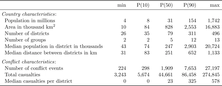
In order to confront our theoretical framework with the data, we assemble a novel cross-sectional
dataset combining a series of raw data sources on ethnic groups and conflict across 24 countries.
It contains information on the location of a total of 3,014 regions, 140 ethnic groups, and 570,023
casualties of conflict from 84,711 conflict events. We begin by describing the data sources, after
which we turn to our sample inclusion criteria. Finally, we describe how we combine the data from
these sources into a single consistent dataset across our country sample.
3.1 Data Sources and Sample Construction
To construct consistent subnational units across countries, we use data from the Global
Adminis-trative District Maps (GADM, 2020) database. In addition to country boundaries, it contains data
on every existing level of administrative divisions from every country in the world. Using
admin-istrative units as opposed to, say, artificial cells has the advantage of being politically meaningful
and often being in line with relevant physical or social boundaries. We focus on the second level of
administrative divisions, typically corresponding to counties in the United States or d´epartements
in France, which we refer to as districts. For countries that do not have a second administrative
level or for whom the number of resulting units is too large for the structural estimation procedure,
we aggregate to the first administrative level, corresponding to the state or province.10
We combine these administrative divisions with data on geocoded conflict from across the globe.
Specifically, we rely on conflict events data from the Uppsala Conflict Data Program (UCDP)
Georeferenced Event Dataset (GED, Stina 2019). UCDP is among the best sources to consistently
document conflict across a large number of countries and periods. We focus on all fatalities over
the years 2000-2018 in all countries included in UCDP.
To consistently identify the spatial distribution of ethnic groups within a country, we draw upon
data assembled in the Geo-referencing Ethnic Power Relations (GeoEPR, see Cederman et al. 2016)
database. The data contains potentially overlapping territories of ethnic group boundaries for 128
countries. Compared to alternative datasets, GeoEPR has the advantage of being recent and
relatively precise, as well as compatible with information on ethnic power relations. We
comple-ment these data with compatible data from the Geographical Research On War, Unified Platform
(GrowUP, see Cederman et al. 2016) project, which we use to measure various country-level and
ethnic group-level characteristics.
10Computational time of our estimator is convex in the number of districts. Hence, we aggregate districts to the
While we are able to observe the extensive margin of the presence of an ethnic group in any
location using the shapefiles from GeoEPR, the data lacks information on the population
frequen-cies, which are a crucial element of our model. To construct population frequencies by district and
ethnic group, we use data from the Gridded Population of the World (GPW, see SEDAC 2018)
database. The data contains estimated population counts for every 2.5-by-2.5 minute land cell on
earth, which corresponds to about 5-by-5 kilometers at the equator.
3.1.1 Sample Inclusion Criteria
To arrive at our 24 included countries, we combine several criteria to restrict the sample of countries
to settings in which our model plausibly applies. In particular, for a country to be included, it
needs to fulfill three conditions: First, we only include countries that have suffered from a relatively
large number of conflict instances, as we need to have enough identifying variation to estimate the
parameters of our model. In particular, we require that a country has experienced at least 200
conflict events according to UCDP. This criterion is fulfilled by 41 countries worldwide.
As a second inclusion criterion, we focus on settings that are characterized by ethnic or religious
conflict – given that we model inter-group strategic interaction rather than, say, class conflict in
a homogenous society. To distinguish ethnic versus non-ethnic conflicts, we draw on the conflict
classification of Kalyvas and Balcells (2010), a widely-used reference on cross-country classification
of conflict. Combining this restriction with the one on the minimal number of conflict events, we
end up with 26 countries in our sample.
Our third and final inclusion criterion concerns the availability of data on the spatial distribution
of ethnic groups within and across countries. Specifically, using the GeoEPR data, we require that a
country has at least two politically relevant ethnic groups in the year 2000. Applying this criterion
further reduces our sample to the final 24 countries.
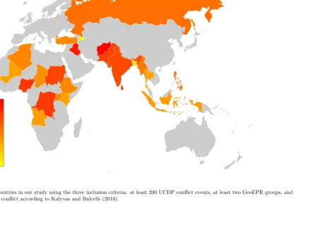
This sample of countries included in the analysis is depicted in Figure 3. Darker colors (red)
represent a higher death toll from conflict over the period 2000-2018, while lighter colors (yellow)
correspond to fewer fatalities. Countries in gray are not part of the sample. We see that our sample
contains various countries from Africa, Asia and the middle East.
3.1.2 Construction of Ethnic Group Population per District
The next challenge is to estimate the population of each ethnic groups residing in a given district,
corresponding to the quantityNig in our model. To the best of our knowledge, there does not exist
census data at the district level that covers in a consistent way a wide number of countries. Hence,
we rely on the combination of GeoEPR and GPW to proxy for the ethnic composition of district
We first estimate district population by summing up population counts of all GPW cells in the
district. We then identify all groups that at least partially overlap with a district and compute for
each group the sum of GPW cells weighted by the share of the district overlapping with the ethnic
group. In case more than one ethnic group is present in a given cell, we divide the population in
the cell equally among them. Since GeoEPR deems some ethnic groups not politically relevant, we
do not count GPW population cells that do not overlap with any ethnic group.
3.2 Example: Iraq
In Figure 4 we show an example country to demonstrate the different types of data we are using.
The map shows the different districts in Iraq. Population is shown as a grayscale layer where darker
colours mean lower density. This is overlayed with the EPR data on the homelands of ethnic groups
which we show as colored areas. The third ingredient to our model is the UCDP violence data
which we depict as red rings, where larger rings represent larger fatality counts. The figure also
illustrates spatial patterns of violence that ethnic interactions will imply. In the North of Iraq most
violence is generated in areas where two homelands of ethnic groups meet. Districts deeper inside
homelands suffer less from violence.
Obviously, our estimation exercise heavily relies on the data that is put into the model. There
are, for example, parts of the country which are not coded as belonging to one group or another.
Furthermore, there are obviously local areas within the EPR homelands where other groups live
which we will not be able to capture with this relatively aggregated data. What we offer is a new
look at existing data through the lens of our model.
3.3 Stylized Facts in the Reduced Form
Drawing on the aforementioned datasets, we start the empirical investigation with a display of
reduced-form stylized facts of ethnic geography and conflict. The rough overall patterns of how
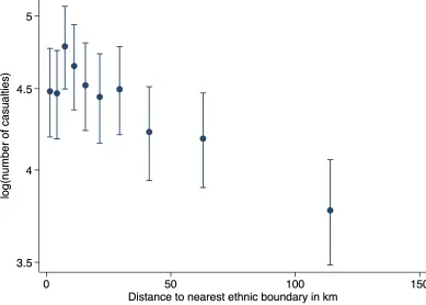
ethnic borders relate to conflict is displayed graphically in Figure 2: Places closer to an ethnic
group boarder are exposed to much larger casualty levels.11
To refine the analysis, we study the role of distance to boundaries between ethnic groups on both
the intensive margin and the extensive margin of conflict in our cross-sectional data. In Table 2, we
regress a binary measure of conflict exposure at the district level (taking a value of 1 if ever between
2000 and 2018 a given district has experienced conflict) as well as the log number of casualties and
conflict events on the distance of the district centroid to the nearest ethnic boundary and district
11Since these reduced-form estimates are not computationally demanding, we show results with a district
population. We gradually introduce country fixed effects, a battery of controls, and dominant group
fixed effects (see table notes).12 This means we are comparing the presence and amount of violence within ethnic groups of each country between districts that are nearer or further from an ethnic
boundary. It turns out that indeed within a given country the most conflict-prone districts are those
located close to ethnic group boundaries and having a large population. Specifically, controlling for
various district-specific features, being 10% closer to an ethnic boundary is associated with a 0.3%
higher probability of any conflict, 1.1% more conflict events, and 1.3% more conflict casualties.
While these associations illustrate the nature of our data and stress well the motivating stylized
facts, we want, in what follows, more specifically confront our novel model to the data, estimating
the structural parameters of our model. In this way, we can not only provide evidence for the
mechanisms proposed in the model – that violence is conducted across space, recruiting fighters to
attack other ethnic groups in the vicinity – but also quantify the structural indices of external and
asymmetric violence discussed in Section 2.4.
4
Estimation
The central expression of our theory is predicted violenceVi∗ =Vi(N,D, θ) in locationias a
func-tion of three components: (a) the spatial distribufunc-tion of groups across locafunc-tionsN= (N1, ...,NG);
(b) the bilateral distance between locations D with elements Dij = distance (i, j); and
parame-ters θ = (α1, ..., αG, µ, κ), where κ captures exponential spatial decay between locations: wij =
exp (−κDij). Using equation (4), we can write this as
Vi(N,D, θ) = G X
g=1
NigW0i(κ) X
k6=g
αkdiag Nµk
W(κ)N−k
We estimate these parameters via maximum likelihood. To this end, denote Yi as the observed
violence in location i, which we assume is an independently and identically distributed draw from
a Poisson distribution with meanVi(N, θ). Under this assumption, the log likelihood function ofθ
given Vi(N, θ) is
L(θ|Y1, ..., YJ,N,D) = J X
i=1
[YilogVi(N,D, θ)−Vi(N,D, θ)−log (Yi!)]
and the estimator is given by
b
θ= arg max
θ∈ΘL(θ|Y1, ..., YJ,N,D)
where Θ⊂RG+2. To ensure that parameter estimates are consistent with our model, we restrict
the parameter space over which we search for a maximum to the positive orthant.13 In this sense, having established the existence of spatial decay in the reduced form, we think of this estimation
exercise as quantifying the degree of spatial decay for a given country. Appendix B.1 shows that
the estimator is able to precisely recover the speed of spatial decay in Monte Carlo simulations.
Since our primary interest lies in the existence and speed of spatial decay of violence, we estimate
κ in two steps. First, we estimate all parameters including µ flexibly. Second, we fix µ to some
value, using the estimates from the first step as initial values. In this way, we can examine how
κ varies across countries in a ceteris paribus fashion: holding constant the marginal cost of local
support, how far does violence travel in a country? We fix µ to various values according to the
results from the first step, including its mean, the mean among those with sufficiently large κ, as
well as at discrete intervals from the mean. We show in Table A.3 that estimates of κ are similar
for various fixed values ofµ.
This two-step procedure also ensures that the parameter vector remains well-identified from an
econometric perspective even whenκ becomes small. As κ approaches zero, group-specific factors
captured inαg become collinear with the cost of local support because they both rely on variation
in country-wide group-specific population, a feature we discuss in Appendix A.3. By fixing µ to
a positive value, we ensure that αg and µ remain separately identified. Despite this potential
collinearity issue in the first step, we show empirically that the estimator converges robustly in the
first step in Appendix B.2.
5
Estimation Results
In this section we describe the results of our estimation. We first provide a brief overview of the
estimated parameters and then discuss in detail how our structural model can open up new avenues
on understanding patterns of violence.
13
Numerically, we restrict the search to an optimum in the positive orthant by taking the logarithm of positive initial values and then exponentiating the parameter values in each iteration. Since the positive orthant is a convex subset ofRG+2, uniqueness of the equilibrium carries through to the estimation, and we show in Appendix B.2 that
5.1 Overview
In Table 3 we provide an overview of the estimates from our model. We find telling evidence for
spatial spillovers. In a bit more than half of the countries we estimate a κ > 0, and the overall
sample mean ofκ >0 is 0.015.14 This means that in many countries violence does not simply take place where target population lives but rather where different ethnic groups are located close to
each other. In contrast, the population living deep inside ethnic homelands (and far from ethnic
borders) is less exposed to violence. These kinds of patterns cannot be simply accounted for by
spatial spillovers of violence – they are driven by the interaction of groups across as space highlighted
by our model.
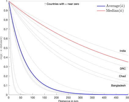
How important is the spatial decay implied by these estimates? To answer this question, we
display the spatial weights corresponding to the κ estimates in Figure 5. The red line represents
the spatial weights of the medianκ and the blue line depicts the meanκ. The other lines illustrate
all individual country estimates with κ > 0. At the mean κ fighters at a location become about
a quarter as effective after 100 km distance. Fighters at the median κ of 0.002 lose effectiveness
much less rapidly and still maintain about half of effectiveness after 350 km.
We also find that our estimates for the average group motivation for conflict, Rg, varies
sub-stantially across groups. These estimates are hard to interpret, however, and we will therefore use
two alternative measures at the country level, vexternal and aasymmetric (see the formal definitions
above). The share of violence coming from outside a district, vexternal, varies significantly across
countries, but even in the lowest decile it is more than 50 percent (see Appendix Figure A.10).
This is an important novel result, because it highlights the importance of separating the origin and
target of violence when analyzing disaggregated violence data. It becomes clear from our estimates
that inter-group interactions across districts play typically a much bigger role than stressed by the
literature on subnational conflict (see literature review above).
Our second summary statistic at the country level is aasymmetric, which lies between 0 and
1, where 0 corresponds to full symmetry, while 1 implies that some groups only inflict fatalities
and other groups only suffer violence. The mean asymmetry is 0.348 which means that in many
countries some groups are estimated to be substantially more aggressive than others. We find a
large amount of heterogeneity in our measure of asymmetry, with some countries being close to
symmetry whereas others are completely asymmetric.
At the group level we provide estimates for Rg, as well as the violence suffered by a group, Vg,
and the violence inflicted by a group, Ag. The three are obviously related, as groups with a high
Rg will inflict more violence. As Vg and Ag are two sides of the same coin, their mean value is
14We round values ofκto zero if they are below 1/10,000. While this is arbitrary, it coincides with the distinction
identical. Interestingly, estimates ofVg are slightly more dispersed than the estimates of Ag: Most
groups suffer some violence and some few groups suffer huge amounts.
5.2 Individual Country Estimates
In Table 4 we show our estimates country by country. It is immediately clear from this list that
spatial interactions are an empirically relevant phenomenon, with 13 out of our 24 countries
dis-playing spatial dynamics with a positive estimate of κ. In several countries, estimates of κ are
fairly large and suggest extreme spatial decay. For example in densely-populated Sri Lanka it is
hard to project violence over wide distances. In contrast, in slightly less than half of the countries
we do not detect a spatial decay of violence, and one can categorize them as having nationalized
violence patterns. These countries include e.g. Afghanistan – where the United States combatted
the Taliban nationwide – and Turkey, Russia and Pakistan which all have a strong national army
engaged in fighting opposition or rebel groups. Hence, given that in these cases national military
campaigns are more prominent than spatial interaction between ethnic groups, we unsurprisingly
find aκ= 0.
In the next two columns of Table 4 we show two measures introduced in section 2.4. The
measure of vexternal captures what share of violence in a district comes from outside the district.
The shares we find here are very large with many countries featuring values close to 1. This provides
an easy benchmark for how important spatial interactions are. In the third column we display our
estimate ofaasymmetric. This statistic is between 0 and 1 where 1 captures a situation where groups
that inflict most casualties do not suffer from any casualties. An interesting feature of the results
here is that countries known for having weak state and military capacities, like e.g. the Democratic
Republic of Congo, have the most symmetric violence. We return to the role of military capacity
in the following section.
Finally, also the estimates for the medianRg at the country level vary considerably, as depicted
in the last column of Table 4. According to our estimates in some countries the overall stakes of
fighting are very high (e.g. in Sri Lanka), while in others they are small (e.g. in India).
5.3 Interpretation
After having displayed above the main estimates, we will discuss in the current subsection the fit
of the model and the various ways in which our model-driven approach allows for new insights to
be derived from the violence data. We start by discussing the fit of our model to the violence data.
Our framework is essentially modeling violence as an interaction between districts. Can such a
As an example, figure 7 shows the (log of) the district estimates for Iraq together with (log of)
the original violence data, revealing a very strong association with a correlation coefficient of 0.853.
It is important to keep in mind that our estimates suggest that 75 percent of this violence came
from outside the respective district, i.e. the majority of violence experienced by ethnic groups in
a district is driven by an interaction with population in other districts – which means that this
strong correlation is not just mechanically driven by district characteristics.
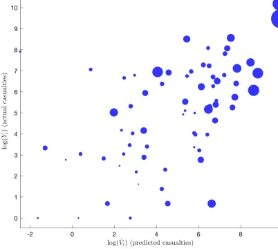
Moving beyond examples, we can aggregate the estimates of local violence to understand
aggre-gate violence. To give an impression of how well our model fits the violence data at the aggreaggre-gate
level, we plot the model fit at the cross country level in Figure 6. On the y-axis we depict observed
violence and on the x-axis we show the numbers coming from our model of spatial violence. The
fit is striking, and implies that our model is able to capture large differences of violence across
countries by modeling local interaction.
Our model provides novel insights beyond the existing macro literature and well-known diversity
indices. To illustrate this, we start by depicting in the left panel of Figure 8 the fit of the log
violence across countries and the ethnic polarization index, as provided by Montalvo and
Reynal-Querol (2005). In line with the findings in this literature (see e.g. Montalvo and Reynal-Reynal-Querol
(2005); Esteban et al. (2012)), there is a remarkably strong positive and significant relationship
between log violence and ethnic polarisation. To highlight what our framework can add to this,
in the right panel of Figure 8 we display the relationship between overall violence and our spatial
model fit, controlling for polarization. What we find is a very robust positive and significant
(p-value=0.008) relationship, showing that the distribution of ethnic groups across space provides
considerable additional explanatory power beyond what is captured by ethnic polarization.
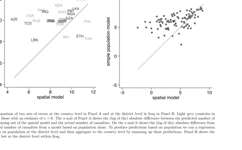
As an additional check for whether our spatial model provides interesting predictive power,
we produce a comparison with a simple model of violence at the district level which only takes
into consideration the population in that district. To make this comparison we focus on the set of
countries for which we estimate κ >0 as we only expect our model of spatial interactions to add
beyond a model based on target population when there are spatial interactions. Figure 9 compares
the error of our spatial model on the x-axis with the error from the population based model on the
y-axis. In Panel A we aggregate the predictions to the country level and show the error at that level.
Countries below the red 45 degree line have a higher error in our model whereas countries above
the line have a larger error in the simple population model. For the large majority of countries
our spatial model provides much better explanatory power. In Panel B we show the example of
Iraq at the district level. Note that errors in the population based model occur for two reasons.
First, a district has a large population but this population is not interacting with the population
relatively small population but is located very close to population from other ethnic groups and
therefore suffers heavily from violence. The low error rates of the spatial model highlights again
the importance of studying interactions between different groups across districts when modelling
violence in some countries.
But how does the model generate this additional explanatory power? Unsurprisingly, a first
factor is the variation in κ across countries. There are obviously many potential drivers of κ.
As shown in the appendix (see Figure A.11), we find reasonable associations with geographic
features like land area of the country, ruggedness and the presence of deserts. This suggests that in
larger countries with smooth terrain spatial distance inhibits fighting less. Obviously, these simple
associations need to be interpreted with great caution, as they are based on only 24 data points.
15 But the approach we propose here suggests the possibility of an alternative way to study the
effect of factors like curfews, barriers, infrastructure or peacekeeping forces which would all be
testable with more fine-grained data on the location of ethnic groups and specific hypotheses on
determinants ofκ in the weighting matrixW.
A key aspect of our model is that it combines the deep parameter estimates of κ, µ and the
group-specificRg, together with the population data, to produce the predictions shown in Figures
6 and 7. One implication of having such a rich set of estimates is that they allow us to separate the
origin and target of attacks. In particular, we are able to back out the group-specific aggressiveness.
In Table 5 we correlate the group-specific violence share and aggressiveness, respectively, with
two key covariates, i.e. group size and group-level oil holdings (from GrowUP (Cederman et al.
2016), see Table notes), that have attracted attention in the literature on group-level conflict (see
e.g. Mayoral and Ray (2017); Morelli and Rohner (2015)). In the first part of the table we have as
dependent variable the share of country-level violence involving a given ethnic group. In column 1
we run a simple regression as one would run it without the estimated model. This simply correlates
the share of violence in the country observed in the homelands of ethnic groups with the group
size and group-level oil holdings. We find that larger groups are on average more often involved
in fighting, and that oil holdings are not statistically significant. These findings carry over to the
columns 2 and 3 where we include country fixed effects and controls.
Do these findings mean that larger groups are more often entangled in fighting because they
are (inherently) more aggressive? Our framework, and in particular columns 4-6 of Table 5, answer
this question, drawing on the aggressiveness statistic provided in equation (6). This variable ranges
between -1 and 1 and captures whether a group attacks more than it is the target of attacks. When
we correlate this variable with group size, the sign switches, and we find a negative relationship, i.e.
15It also needs to be kept in mind that our analysis here should only be regarded as a first step towards unwrapping
that larger groups are on average less aggressive. We also find that oil-rich groups are on average
more aggressive.
Asymmetry of violence at the country level should relate to how strong the different ethnic
groups are and whether incumbents can control a strong military force – a group which is in control
of a stronger state can more easily project violence across the country and targets and origins of
violence will coincide less geographically. We would then, conditional on observing violence, expect
a larger degree of asymmetry in countries with stronger militaries as these are directed against
non-incumbent groups. And, indeed, we find a positive association between military expenditure
per capita and asymmetry at the country level.16 We also find a strong positive link between GDP
per capita and asymmetry which is in line with broader ideas on state capacity proposed in Besley
and Persson (2010). Both associations are shown in Appendix Figure A.12. Note, that this holds
despite the fact that our proxies of state capacity and overall levels of violence are not significantly
associated in our dataset.
These results demonstrate the potential of our model-based approach to provide new insights
into the origins of violence and on which countries and regions can be expected to become most
violent if conflict were to break out. This being said, it is of course crucial to interpret these
correlations with much caution, as omitted variables remain a valid concern.
5.4 Robustness
We run several robustness checks in the appendix. Most importantly, we check whether our
esti-mates of the role of spatial decay are a function of whether we fixµand whether the level matters.
In Appendix Table A.3 we show that estimates ofκare remarkably robust across different estimates
of µ. This further justifies fixingµ to be able to make ceteris paribus comparisons.
Given that casualties are measured noisily in UCDP, we also use the number of conflict events
itself as our outcome of interest. This yields qualitatively similar estimates ofκin Appendix Table
A.3, both with fixed and flexible µ. We conclude that patterns of spatial decay are indeed mostly
driven by structural features relating the distribution of ethnic groups to the frequency of conflict
across locations, as opposed to the exact choice of proxy for conflict intensity in a location.
6
Counterfactuals
One of the key advantages of estimating our structural model over reduced form estimates is that we
can use it to run counterfactual analyses in which we change key parameters of the model. In Table
6 we run four counterfactual experiments. First, we half κ: such a policy could be thought of as
16
increasing infrastructure projects or facilitating ethnic targeting through information technologies.
While such measures may have large economic benefits, they may also under some conditions
facilitate ethnic violence. Strikingly, this experiment produces dramatically different effects across
countries. In Algeria or Kenya violence may increase more than sevenfold, whereas in Bangladesh
or Chad it would not even have doubled, and in Angola the simulation suggests that violence would
have increased by just over 20 percent. Our take on this is not that such infrastructure projects
should necessarily be put on hold in high-risk countries, but rather that the government may want
to accompany them with pacification efforts (see discussion of columns 3 and 4 below).
In column 2 we simulate a policy which doubles the spatial decay parameterκ. This is a policy
which can be thought of as – during peaks of violence – severing or controlling transport links
or imposing curfews. We find a dramatic fall of violence in most countries. Interestingly, this is
the sort of reaction that has been found by scholars who have analyzed the role of the Covid-19
pandemic on armed conflict (see e.g. Berman et al. 2020). The reduced mobility of armed actors
seems to have indeed reduced violence.
In column 3 we show an experiment in which the ethnic group with maximum Rg is pacified,
i.e. where the group’sRg is set to 0. This will have the biggest impact in countries where one group
was engaging in a lot of violence. Reducing the stakes of fighting could be achieved for example
through power-sharing agreements that result in reducing the edge between being inside versus
outside the government (see Mueller and Rohner 2018). Column 4 performs a related experiment –
setting the conflict prize of all groups with an above-median estimated conflict prize to the median
– and again finds a strong pacification potential of such measures.
7
Conclusion
The aim of this article has been to introduce the concepts of space and distance into a canonical
model of conflict, in order to understand the drivers of conflict from a distribution of violence and
population across space. This approach has been extremely successful in other areas like trade
(Fajgelbaum et al., 2017; Donaldson, 2018) by integrating trade models with empirical measures
of trade costs to understand the distribution of economic activity across space. However, coercion
follows a very different logic than the exchange of goods and the conflict literature has up to now
typically followed the approach of using contest functions as a way to model conflict effort (see e.g.
Konrad 2009). In the current contribution we have brought the idea of spatial interactions into this
class of models with the goal of studying situations in which the drivers of violence are separated
spatially from the violence.
coun-tries – highlighting a substantial between-country heterogeneity that is associated among others
to topological factors. In more than half of the countries in our sample inter-group distance plays
a key role for violence, and in the median country having 350 km larger distances between given
groups cuts fighting by half. Our estimates allow for tracing back the origin of violent attacks and
carrying out a series of counterfactual experiments. Beyond estimating the role of space separately
for each country in our sample, our model also permits to forecast potential implications of specific
shocks to the model parameters. For example, the lockdowns put in place in the face of the current
covid-19 pandemic make it typically harder for anyone (fighters included) to travel across space,
resulting in higher κ, which in turn would typically reduce the scope for ethnic violence. This is
consistent with recent empirical evidence (Berman et al., 2020).
Several avenues seem promising for future research: First, our setting entails the possibility of
building joint models of coercion and voluntary contract in space which may foster our
understand-ing of the distribution of economic activity in the least developed countries that are often plagued
by armed conflict.17 Further research in this direction is very much encouraged. Second, it would be interesting to extend the model to allow for beneficial effects of inter-group interaction (e.g. with
trust-building `a la Rohner et al. 2013b). Third, we warmly encourage studies that build on the
current framework to study other phenomena than conflict where spatial heterogeneity of intensity
and local interactions play an important role. Migration, for example, is most attractive where
rich areas are close to poor areas. Other examples are topics in electoral politics, such as the study
of local campaigning in national elections, or public health policies such as anti-AIDS campaigns.
Finally, for specific cases with more fine-grained population and violence data it would be
possi-ble to study specific policies to promote or hinder movement such as barriers or the presence of
peacekeepers. A model which integrates such policies into the spatial decay matrix and tests their
impact inside the model would provide a completely new avenue of research into the effectiveness
of such measures.
17See Dal B´o and Dal B´o (2011) and Gonzalez et al. (2012) for existing joint models of coercion and voluntary