Welfare Effects of
Short-Time Compensation
Helge Braun
University of Cologne
Bj¨
orn Br¨
ugemann
VU University & Tinbergen Institute
Klaudia Michalek
University of Cologne
April 2013
Abstract
1
Introduction
All advanced economies operate unemployment insurance (UI) systems. In addition,
many countries run short-time compensation (STC) schemes, which pay benefits to
work-ers that have not lost their job entirely but are working reduced hours. In contrast to
UI, however, STC is far from universal among advanced economies: the OECD is about
evenly split between countries with and without STC. The political debate about the
desirability of STC has recently been reignited by the severe labor market difficulties of
the Great Recession.
In this paper we examine the welfare effects of STC, pursuing the following two
questions. First, we ask whether introducing STC can improve on UI. As a benchmark
we consider a system that limits itself to UI, choosing the level of UI optimally. Starting
from this benchmark, we examine whether it is possible to raise welfare by introducing
STC for a given level of UI. Second, we ask how STC and UI should be combined
optimally.
We study these questions using a static model in which firms experience idiosyncratic
profitability shocks. Labor input at the firm level can vary both at the extensive and the
intensive margin. Optimal hours per worker are determined by trading off fixed costs of
working against increasing marginal disutility of working longer hours. For simplicity we
abstract from the distinction between employers and employees, and consider firms that
are jointly owned and operated by a group of identical risk averse individuals. Firms can
adjust to adverse profitability shocks on both margins, that is, through layoffs, through
work sharing in the sense of a reduction of hours per worker, or a combination of both.
We assume that firms have only limited access to external private insurance against
prof-itability shocks. This implies that government-provided insurance can improve welfare.
We consider a government that has access to two policy instruments. First, UI, which
is modeled as providing a payment for each worker that is working zero hours. Second,
STC, which is modeled as providing a payment for each hour by which working time is
reduced below some threshold of normal hours.1
The welfare effects of UI in this type of environment are well understood: it provides
valuable insurance at the cost of distorting labor inputs. First, UI reduces labor input
below the efficient level as in Feldstein (1976), because firms do not internalize the
ef-fects of layoffs on the government’s budget. Second, UI biases the mode of labor input
reductions towards layoffs and against work sharing. Given this, there are two channels
through which STC could improve on a system that is limited to UI. First, it could
counteract the distortion of the composition of labor input induced by UI. Second, it
could directly improve the provision of insurance by better aligning insurance payments
with the level of distress of the firm. In particular, UI does not provide any insurance
payments to firms that adjust to a decline in profitability solely through work sharing,
that is, by reducing hours without any layoffs.
We first provide an analytical examination of how labor input choices of firms respond
to profitability shocks in the presence of UI and STC. This analysis focuses on the
trade-off between hours and employment. It shows how STC can eliminate the distortion of the
composition of labor input induced by UI. It also yields an insight that is important for
the direct insurance role of STC: comparing two firms that have experienced uninsured
declines in profitability and engage in layoffs, the firm with the larger decline in
profitabil-ity will have higher hours per worker. This holds because the scarcprofitabil-ity of consumption
in more distressed firms implies that marginal utility of consumption is high relative to
the marginal disutility of increasing hours. This induces firms to move towards higher
hours in order to economize on fixed costs when profitability is low. This mechanism
is amplified by UI, which acts as an additional fixed cost of employment. This result
implies that in terms of insurance, STC is poorly targeted among firms that engage in
layoffs: more distressed firms may not take up STC because it is optimal for retained
workers to work relatively high hours.
We then turn to computational experiments to examine the welfare effects of STC
quantitatively. In our calibration we leave unidentified one feature that turns out be
critical for the desirability of STC, namely the extent to which firms are insured against
profitability shocks in the absence of public insurance. While the theory suggests that the
extent of insurance can be identified from the response of labor inputs to adverse shocks,
implementing this identification approach is beyond the scope of this paper. Instead, we
consider two scenarios that differ in the extent to which shocks are privately insured. Our
and it is always uninsured. We interpret this as a permanent shock. The second type of
shock is less severe, and firms can adjusts through layoffs and/or changes in hours. We
interpret these shocks as temporary. The two scenarios differ in whether this second type
of shock is privately insured.
In the first scenario firms are insured perfectly against temporary shocks. This
sce-nario corresponds to the view expressed by Feldstein (1976, p. 941), who abstracts from
worker risk aversion in his theoretical examination of temporary layoffs motivated by the
observation that “the spells of unemployment are both temporary and brief”. Thus only
permanent shocks are uninsured in this scenario. This means that only UI can provide
insurance, and the only potential role of STC is to mitigate distortions caused by UI.
We carry out three policy experiments in this scenario. First, we determine the optimal
level of UI under the restriction that STC is not available. Second, we determine the
optimal level of STC given this level of UI. Third, we determine the optimal combination
of STC and UI. In the second experiment we find that it is optimal to introduce STC,
and that the optimal level of STC (given the level of UI) results in a large increase in
employment and a sizable improvement in welfare. In the third experiment we find that
the availability of STC makes it optimal to provide more generous UI. This is intuitive,
given that STC provides a way to mitigate the distortions of UI. In this sense STC
indi-rectly enables better insurance. While we find that positive STC is desirable, our results
indicate that it should be less generous than UI.
In the second scenario both temporary and permanent shocks are uninsured in the
absence of public insurance. Now STC has a direct effect on insurance, but this effect is
negative. As discussed above, the reason is that distressed firms optimally choose to have
high hours per worker and to forego STC. Furthermore, since it is this set of firms for
which UI induces excessive layoffs, STC also loses the ability to counteract this distortion.
Consequently the introduction of STC is not optimal in this scenario.
Overall, our results indicate that the extent to which temporary profitability shocks
are insured is a key determinant of the optimality of STC.
Our model builds on the analysis of UI and STC provided by Burdett and Wright
(1989, henceforth BW). BW examine how UI and STC distort labor inputs. Their main
results are that UI causes inefficient layoffs, while STC does not cause inefficient layoffs
but induces inefficient hours. BW do not study the welfare implications of UI and STC
The paper is organized as follows. We introduce the model in Section 2. In Section 3
we first derive the allocations for autarky and first-best, and then characterize the
alloca-tion for a given system of UI and STC. Secalloca-tion 4 contains the computaalloca-tional experiments,
the robustness of our results ins examined in Section 5, and Section 6 concludes.
2
Model
There is a single firm with a continuum of positions of massN. All positions are initially filled by risk averse workers that are ex ante identical. We assume that the firm is jointly
owned and operated by these workers. We normalizeN = 1.
Technology. The firm’s production function is
xf(nh)−nF
where n denotes the mass of workers working strictly positive hours, and h denotes the number of hours worked by each of these workers. Here x parametrizes the profitability of the firm. It is subject to stochastic shocks that can be of technological or other origin,
and which will be specified in more detail below. The function f : [0,+∞) → [0,+∞) is strictly increasing and strictly concave. It is twice continuously differentiable and
satisfies limnh↓0f0(nh) = +∞. Working strictly positive hours is associated with a fixed
cost F ≥ 0 for each worker, thus the total fixed costs incurred by the firm are given by
nF.
Shocks and Limited Access to External Insurance. Profitability x is subject to stochastic shocks. Specifically, it is a function x(s) of the state s ∈ S. The probability of state s is denotedθ(s). The firm has limited access to external insurance. To capture this in a simple way we allow for two sets of shocks, insured and uninsured. Specifically,
we partition the state space into two subsets S = SI ∪SU, and assume that the firm
can perfectly insure itself across realizations in SI, but cannot insure itself at all for
realizations in SU. This setup allows us to accommodate the two scenarios we will
consider in our computational experiments. In the first scenario the set SU only consists
of a single statesP with x(sP) = 0, so that the firm shuts down production in this case.
We interpret this as a permanent shock that breaks the attachment between the workers
setSI in this scenario. In the second scenario all shocks, both permanent and temporary,
are in the uninsured setSU.
Preferences. The expected utility of a worker is given by
X
s∈S
θ(s){n(s)[u(w(s))−v(h(s))] + (1−n(s))u(b(s))}.
The expectation is taken with respect to the state s since this is the only source of uncertainty. The firm chooses labor inputs conditional on s. If total employment in state s is n(s), then n(s) is also the probability that a given worker is working positive hours. Utility is separable between consumption and hours. Here w(s) and b(s) denote the consumption levels of workers with positive and zero hours, respectively, and the
function u is twice differentiable, strictly increasing, and strictly concave. The common level of hours worked by those with positive hours in state s is denoted h(s). The disutility of working h hours is given by v(h). The function v satisfies v(0) = 0, is twice continuously differentiable differentiable, strictly increasing, strictly convex, and satisfies
the Inada condition limh↑hmaxv0(h) = +∞ for somehmax >0.
Differences from BW. Our model largely follows BW. There are some differences,
however. First, BW assume that the firm is owned by a risk averse employer, and they
analyze optimal risk sharing between workers and the employer. The assumption of
owner-operators simplifies the analysis by allowing us to ignore considerations of risk
sharing between workers and employers, which are not our focus.
Second, our production function differs slightly. BW allow for a more general function
of hours and employment. More importantly, they impose an assumption that rules
out any fixed costs associated with employment. Specifically, they assume that if two
combinations of hours per worker and employment yield the same total number of hours,
then the combination with higher employment delivers higher output. The opposite is
true in our specification when the fixed costF is strictly positive. In their analysis, this assumption insures that layoffs are never optimal in the absence of policy.
Finally, we simplify the analysis by assuming additively separable preferences over
3
Firm Behavior and Allocations for Given Policy
In this section we analyze optimal firm behavior and characterize the resulting allocation.
We begin with the benchmark allocations of first best and autarky, and then turn to the
allocation for a given system of UI and STC.
3.1
First Best
First we examine the allocation that would arise if the firm were able to obtain perfect
insurance across all profitability shocks.
Throughout the paper we maintain the assumption of perfect risk sharing within
the firm. Together with the separability of utility between consumption and hours, this
implies that consumption of workers with positive hours and workers with zero hours
is equalized, that is, w(s) = b(s). Using this property to simplify the objective, the first-best allocation is obtained as the solution to
max
c(s),n(s)∈[0,1],h(s)∈[0,hmax]
X
s∈S
θ(s){u(c(s))−n(s)v(h(s))}
s.t. X
s∈S
θ(s){x(s)f(n(s)h(s))−n(s)F −c(s)}= 0.
The first-order condition for consumptionc(s) is
u0(c(s)) =λ (1)
whereλ denotes the multiplier associated with the constraint. This first-order condition implies that marginal utility of consumption and thereby consumption are equalized
across states.
Next we will discuss the first-order conditions for the choice of labor inputs. There
are two cases to consider, depending on whether the employment constraint binds.
Case 1: n(s) ≤ 1 slack. For this case it is convenient to consider the first-order condition associated with a variation that reduces employment while keeping total hours
constant:
u0(c(s))F =h(s)v0(h(s))−v(h(s)). (2)
While we already know that marginal utility is equalized across states here, we continue to
autarky. To interpret this condition, first consider the function of hours that appears on
the right-hand side:
V(h)≡hv0(h)−v(h).
It gives the increase in the expected disutility of working associated with this variation.
If an additional worker is laid off, this reduces disutility by v(h). Total hours fall by h. To keep total hours constant, these hours must be reallocated to the remaining workers,
which increases disutility by hv0(h). The strict convexity of v implies that the function
V(h) is strictly increasing. Condition (2) can now be written as
u0(c(s))F =V(h(s)). (3)
Since the variation leaves total hours unchanged, gross output f(n(s)h(s)) remains un-changed while net output increases due to a drop in fixed costs. The left-hand side gives
the increase in utility due to this reduction in fixed costs. Importantly, condition (3) does
not directly depend on profitabilityx. Since marginal utility of consumption is equalized across states, it follows that hours do not vary across states with interior employment.
The first-order condition for employment is
u0(c(s)) [x(s)f0(n(s)h(s))h(s)−F] =v(h(s)). (4)
If x(s) is strictly positive, then employment n(s) is strictly positive due to the Inada assumption imposed on f. Since both hours and marginal utility due not vary with profitability, it follows from equation (4) that employment is increasing in profitability
across states in which this case applies.
Case 2: n(s) ≤ 1 binds. With the employment constraint binding, hours are deter-mined by the condition
v0(h(s))
u0(c(s)) =x(s)f 0
(h(s)). (5)
The left-hand side is the marginal rate of substitution between leisure and consumption,
and the right-hand side is the marginal product of hours when employment equals one.
Since marginal utility is constant across states, it follows that hours are increasing in
profitability across states in which this case is applicable.
Summary. Case 1 applies for low levels of profitability, Case 2 for high levels of
em-ployment increases. Eventually all workers are employed and switch from constant to
strictly increasing.
3.2
Autarky
In autarky the firm does not have any insurance for realizations of the shock in the
uninsured setSU. Thus the autarky allocation solves
max
c(s),n(s)∈[0,1],h(s)∈[0,hmax]
X
s∈S
θ(s){u(c(s))−n(s)v(h(s))}
s.t. X
s∈SI
θ(s){x(s)f(n(s)h(s))−n(s)F −c(s)}= 0
and c(s) = x(s)f(n(s)h(s))−n(s)F ∀s∈SU.
The first constraint now reflects that insurance occurs only across states in the insured set
SI. The second constraint reflects that in other states consumption must equal output.
The problem of choosing the optimal allocation across the insured states does not
interact with choosing the allocation for the remaining states. Furthermore, the former
problem is identical to the first-best problem. Thus here we only need to discuss the
problem of choosing the allocation for the uninsured states.
Substituting the second constraint into the objective, for each state s ∈SU the firm
solves
max
c(s),n(s)∈[0,1],h(s)∈[0,hmax]{u[x(s)f(n(s)h(s))−n(s)F]−n(s)v(h(s))}.
Again there are the same two cases for employment, but the qualitative behavior of
labor inputs within the regions with positive employment is modified by the absence of
insurance.
Case 1: n(s)≤1 slack. Across states in this region consumption and hours are linked through equation (3). Marginal utility is decreasing in profitability due to the absence
of insurance, hence hours are also decreasing in profitability. This is driven by the fact
that the fixed cost of employing a worker is incurred in terms of the consumption good,
and economizing on consumption becomes relatively more important when profitability
is low.
the marginal utility of consumption is now decreasing in profitability, which works in the
opposite direction. Thus the total effect of higher profitability on hours across states in
this region depends on the relative strength of substitution and income effect.
Summary. In the first-best allocation it is guaranteed that employment is monotone
increasing in profitability. In contrast, here the effect of profitability on employment
depends on the relative strength of income and substitution effect, so depending on
parameters it is possible that employment moves from case 2 to case 1 as profitability
increases.
3.3
Unemployment Insurance and Short-Time Compensation
We now specify the two policy instruments, and study the firm problem in the presence
of policy.
3.3.1 Parametrization of Policy
In modeling the two policy instruments we largely follow BW. UI takes the form of a
paymentgU I to workers with zero hours worked. STC takes the form of a paymentgST C
to employed workers for every hour that hours worked fall short of some “normal” level of
hours H. BW assume that the government balances the budget of the insurance system by imposing a lump-sum tax on firms.2 For our main results we depart from BW and
assume that the budget is balanced through a proportional taxτ on total hours nh. Our motivation is that this specification is closer to the observed financing of unemployment
insurance through payroll taxes.3 We will compare our main results to lump-sum taxation
in the robustness analysis.
With the proportional tax on total hours, the net transfer received by a firm with
employment level n and hours per worker h is given by
(1−n)gU I +nmax[0, H−h]gST C−τ nh.
2BW assume that financing occurs in part through experience rating. It is easy to see that experience rating is redundant in the model, as it is equivalent to lower values of the insurance instrumentsgU I and
gST C. This is precisely the point why BW consider experience rating: for given values ofgU IandgST C,
experience rating can be used to eliminate any effects of UI and STC on the allocation of resources, including any distortionary impact on labor inputs. In contrast, our objective is study the effects of gU I and gST C on the allocation when firms’ access to insurance is limited, and given this purpose it is
redundant to allow for experience rating.
It is instructive to rearrange this schedule to isolate an intercept, a coefficient onn, and a coefficient on nh:
(
gU I −n[gU I −HgST C]−nh[gST C+τ], h < H,
gU I −ngU I −nhτ , h≥H.
(6)
Consider first the subsidy received by a firm with below-normal hours h < H. The first term is the intercept and represents the transfer received by a firm that shuts down
production: it receives the unemployment benefit gU I for all of its workers. The second
term is linear in employment n, and the coefficient captures the additional fixed cost of employment that is induced by policy: switching a worker from zero hours to a positive
but negligible amount of hours results in the loss of unemployment benefitsgU I, which is
offset partially or fully by the fact that the worker becomes eligible for the maximal STC
benefit HgST C. The last term is linear in nh and shows that an increase in total hours
by one results in a reduction in the net transfer consisting of the sum of the proportional
tax τ and the STC benefitgST C.
As hours cross the normal threshold H, the coefficient on n rises to gU I since STC
no longer offset the policy-induced fixed cost, and the coefficient on nhdrops to the tax rate τ.
Our policy specification differs from BW in two important ways, apart from a different
tax instrument balancing the budget. First, BW sidestep the issue of normal hours by
setting H = 1 and adopting preferences for which the maximal level of hours is also
hmax = 1. This insures that hours are always below the “normal” level. This simplifies
the analysis and does not matter for their main results. In our analysis we permit
H < hmax, and in our computational experiments we set H equal to the average level of
hours. The possibility of hours exceeding the normal level turns out to be relevant for the
welfare effects of STC. Second, BW restrict attention to two regimes: an American regime
in which gST C = 0, and a European regime in which UI and STC are equally generous,
that is, HgST C = gU I. In our analysis we allow any gST C as long as HgST C ≤ gU I. In
the computational experiments it turns out that usually it is not optimal to make STC
3.3.2 Firm Problem with Policy
The firm problem with policy is
max
c(s),n(s)∈[0,1],h(s)∈[0,hmax]
X
s∈S
θ(s){u(c(s))−n(s)v(h(s))}
s.t. X
s∈SI
θ(s)x(s)f(n(s)h(s))−n(s)−c(s)
X
s∈SI
+ (1−n)gU I +nmax[0, H −h]gST C −τ nh = 0
and c(s) =x(s)f(n(s)h(s))−n(s)F
c(s)+ (1−n)gU I +nmax[0, H −h]gST C−τ nh ∀s∈SU.
We will now discuss the first-order conditions for labor input choices. There are four cases
to consider, depending on whether the employment constraint is binding and whether
hours are below or above normal.
Case 1: n(s) ≤ 1 slack and h(s) < H. Consider again the variation of reducing employment while keeping total hours constant. This yields the following generalization
of equation (3):
u0(c(s))[F +gU I −HgST C] =V(h(s)). (7)
The new term on the left-hand side gU I −HgST C is the additional fixed cost associated
with policy, as identified in the upper branch of equation (6). If employment is reduced
by one worker, this results in the gain of unemployment benefits gU I. Since h(s) < H
this worker loses [H−h(s)]gST C in STC payments. Furthermore, since total hours are
kept constant in this variation, hours by other workers are increased by h(s), resulting in a further reduction of STC payments by h(s)gST C. Thus the gain of gU I is offset by
a combined loss of HgST C in STC payments. UI distorts the allocation in the direction
of lower employment and higher hours per worker by acting like an additional fixed cost.
STC counteracts this distortion and eliminates it entirely if UI and STC are equally
generous, that is, if HgST C =gU I.
The first-order condition for employment is the following generalization of equation
(4):
Policy instruments appear in this condition in two ways. First, there is again the
addi-tional fixed costgU I −HgST C. Second, gST C adds to the tax on total hours.
Marginal utility of consumption is constant across insured states, hence hours are
con-stant as in the absence of policy. Also as in the absence of policy, hours are decreasing
in profitability across uninsured states, that is, hours per worker are higher in distressed
firms. In autarky this is driven by the assumption that the fixed cost of employing a
worker is incurred in terms of the consumption good. Here this is amplified by
unem-ployment insurance, which increases the effective fixed cost that is incurred in terms of
consumption.
Case 2: n(s)≤1binding and h(s)< H. The first-order condition determining hours is the following generalization of equation (5):
v0(h(s))
u0(c(s)) =x(s)f 0
(h(s))−(gST C+τ). (9)
STC distorts hours downwards in firms that employ all workers. At the margin and
holding constant the tax rate τ, an increase ingU I does not affect labor input choices of
firms for which this case applies.
Case 3: n(s) ≤ 1 slack and h(s) > H. With hours above the eligibility threshold for STC, the variation of reducing employment while maintaining total hours yields the
following generalization of equation (3):
u0(c(s))[F +gU I] =V(h(s)). (10)
In contrast to equation (7), here the distortion induced by unemployment benefitsgU I is
not mitigated by STC. The first-order condition for employment is
u0(c(s)) [x(s)f0(n(s)h(s))h(s)−(F +gU I)−h(s)τ] =v(h(s)).
In comparison to equation (8), STC has dropped out of the fixed cost as well as the
Case 4: n(s) ≤ 1 binds and h(s) > H. The first-order condition determining hours is the following generalization of equation (5):
v0(h(s))
u0(c(s)) =x(s)f 0
(h(s))−τ . (11)
In contrast to equation (9), hours are not distorted by STC, but they remain distorted
by the proportional tax on total hours.
3.4
Discussion
We conclude this section with a discussion of the qualitative features of the allocations
derived above that will be important determinants of the welfare effects of UI and STC.
The lack of external insurance is the only friction in this model. Achieving the
first-best allocation would require non-distortionary transfers toward firms that experience
uninsured adverse shocks to profitability. The problem of the government in our model,
whose policy instruments are limited to UI and STC, is to approximate the first-best
schedule of transfers while minimizing the distortions of the composition and level of
labor input induced by these policy instruments.
Distressed firms in the model, that is, firms experiencing uninsured declines in
prof-itability, tend to have low employment. High marginal utility of consumption pushes the
composition of labor input in the direction of high hours and low employment, hence
employment is low unless income effects are very strong. Low employment in distressed
firms implies that UI is targeted well from an insurance perspective. However, it transfers
resources to distressed firms at the cost of distorting both the level and the composition
of labor input. Introducing STC affects welfare through two channels. First, it can
mitigate and even eliminate the distortion of the composition of labor input induced by
UI. Second, it directly modifies the provision of insurance. Yet this effect reallocates
resources in the wrong direction among distressed firms that engage in layoffs, since more
distressed firms have higher hours per worker within this group of firms, hence they may
not qualify for STC and receive less STC if they do. In this sense STC can be poorly
4
Computational Experiments
4.1
Calibration
We calibrate the model using US evidence. The functional from for gross output is:
f(nh) = (nh)α.
We set α = 23, implicitly assuming that capital cannot be adjusted in response to prof-itability shocks. For preferences we assume
u(c) = c
1−σ−1
1−σ ,
v(h) =η h
1+ψ
1 +ψ.
The parameter η only affects the level of hours, so we can use it to normalize average hours to one. We also set the level of normal hoursH to one, so it is assumed to coincide with averages hours in the calibration. We set the coefficient of relative risk aversion to
σ = 2, in the lower middle part of the plausible range (about one to five) indicated by microeconomic evidence. The parameter ψ is the inverse of the Frisch elasticity of labor supply. Based on the recent survey of the microeconomic evidence in Hall (2009), we set
ψ = 1.43 to obtain a Frisch elasticity of 0.7.
Concerning profitability shocks we have to separately specify the distribution of
in-sured and uninin-sured shocks. We assume that there is always a shock sP with x(sP) = 0
that leads to a shutdown of production and is uninsured. This is interpreted as a
per-manent shock that breaks the attachment of workers to the firm. We assume that the
probability of this shock is θ(sP) = 0.06, so that 6% of workers are affected by
non-temporary layoffs. The presence of this group of workers is the primary reason why UI
can improve welfare in the model. With complementary probability 1−θ(sP) the firm
receives a less severe shock, which we interpret as a temporary shock. It is drawn from
a log-normal distribution with standard deviation ofσx= 0.1 (discretized using 250 grid
points) and mean normalized to one. As discussed above, in this paper we make no
attempt to identify the extent to which firms are insured against these shocks in the
absence of public insurance. Rather, we consider two scenarios. In the first scenario we
assume that temporary shocks are insured, that is, they are part of the set SI. In this
mitigating labor-input distortions caused by UI. In the second scenario we assume that
temporary shocks are uninsured, that is, all states are in SU and SI is empty.
We assume that the calibrated economy has UI but no STC. This leaves two
parame-ters to be calibrated. The per-worker fixed costF and the level of unemployment benefits
gU I. These parameters are jointly calibrated to match the following two targets. First,
we target that 2% of workers are unemployed due to a temporary shock. This means
that total unemployment is 8%, and 25% of the unemployed are on temporary layoff.
This target is chosen based on the empirical prevalence on temporary layoffs, defined
as unemployment in spells which end with the unemployed person being rehired by the
same employer. On average, the fraction of the unemployed in the US that is reported
in the CPS to be on temporary layoff is 14%.4 Based on the SIPP, Fujita and Moscarini
(2012) report that a group of unemployed workers of at least equal size is not classified
as on temporary layoff, but ultimately returns to the same employer.5 Second, we target
that the unemployment benefit gU I amounts to 25% of average consumption of workers.
The latter is our definition of the replacement rate for this model. Recall that experience
rating is neutral in our model andgU I corresponds to the actual subsidy provided by the
government. To map our model to replacement rates in the US, we need to eliminate the
non-subsidy component of observed replacement rates associated with experience rating.
Topel (1983) reports that on average the subsidy component is 31% of earnings.
Further-more, notice that in our model workers jointly own and operate firms, hence implicitly
their average consumption reflects income from both wages and profits. This leads us to
adopt the somewhat lower target of 25%.
We associate parameters with targets as follows. Equation (10) shows that in the
absence of STC, the total fixed cost in terms of consumption of working positive hours
is given by F +gU I. The higher these fixed costs, the more attractive it is for the firm
to have low employment and high hours. Thus the target for the fraction of temporary
layoffs identifies the sum F +gU I. The target for the replacement rate then identifies
how this sum is composed of physical fixed costs and unemployment insurance.
The calibration is summarized in Table 1. The policy parameter gU I is pinned down
quite directly by the replacement rate target. The parameter for which the approach is
4The average is taken over the years 1967-2012.
most indirect is the per-worker fixed cost F: to generate that 2% of all workers are on temporary layoff, this fixed cost must absorb about 12 percent of output.
4.2
Welfare Effects of STC when Temporary Shocks are Insured
We use the calibrated model to carry out the following sequence of three policy
experi-ments. First, we restrict the set of policy instruments to unemployment insurance and
determine the welfare-maximizing level of gU I. We refer to this level of benefits as gU I∗ ,
and also use gU I∗ to label this experiment. Second, we determine the optimal level of
gST C holding constant gU I at gU I∗ . Thus by construction the introduction of gST C in this
way does not improve the level of consumption of workers affected by the uninsured
per-manent shocks in this experiment. Therefore, to the extent that STC does improve the
allocation, it can only do so by mitigating the distortion of labor inputs induced by U I. We refer to the corresponding level of STC and also the entire experiment as gST C∗ |g∗
U I
to indicate that gST C∗ is optimal given that UI is fixed at gU I∗ . Finally, we determine the welfare-maximizing combination of gST C and gU I. We denote this pair as (g∗∗U I, g
∗∗
ST C).
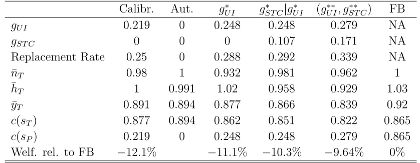
Results from these experiments are displayed in Table 2, along with the allocations for
the calibration, the first-best and autarky as points of reference. For each allocation,
the first three rows show the values of the policy instruments gU I and gST C, along with
the replacement rate implied by the value ofgU I (defined as gU I as a fraction of average
consumption). The next three rows show the average of employment and hours across
temporary shocks, denoted ¯nT and ¯hT, respectively, along with average output ¯yT
(em-ployment, hours, and output are all zero in the single non-insured state by construction in
this calibration). The next two rows show consumption levels for after temporary shocks
(consumption is equalized across all insured states) and the single permanent shock state,
denoted by c(sT) and c(sP), respectively. The final row shows, for each allocation, how
much lower welfare is compared to the first best, in consumption-equivalent terms.6
The results for experiment g∗U I show that it is optimal to make UI slightly more generous than it is in the calibration. This is despite the fact that the modest increase
ingU I from the calibrated level to gU I∗ would more than triple the number of workers on
temporary layoff.
The results for experiment g∗ST C|g∗
U I show that it is optimal to introduce a modest
amount of short-time compensation when UI is held fixed at gU I∗ . Introducing this level of STC is quite effective in reducing temporary layoffs, roughly to the level targeted in
the calibration. However, hours per worker drop substantially, so that output is lower
than in the gU I∗ experiment. The optimal level of STC is lower than gU I∗ , hence it is not optimal to completely eliminate the distortion of the composition of labor input.
The optimal combination of UI and STC is associated with substantially more
gener-ous UI than what is optimal if STC is not available: the benefit increases by 13% (from
0.248 to 0.279), which corresponds to an increase in the replacement rate from 29% to
34%. The mechanism underlying this result is that STC counteracts the distortion of the
composition of labor input associated with UI. As a consequence, the availability of STC
makes it optimal to offer more generous UI. As in experiment gST C∗ |g∗
U I it is optimal to
make STC less generous than UI, so the distortion of the composition of labor input is
not eliminated entirely.
The overall welfare gain of moving fromg∗U I to (g∗∗U I, gST C∗∗ ) corresponds to about 1.5% of first-best consumption. About half of this gain can be obtained by moving togST C∗ |g∗
U I.
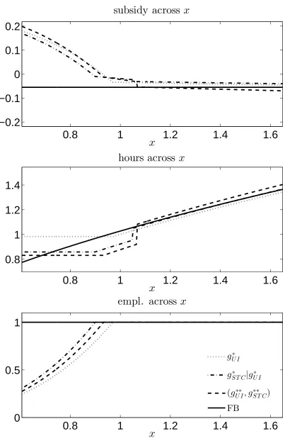
Figure 1 illustrates how policy affects labor inputs across realizations of the temporary
shock. The top panel shows the net transfers firms at different levels of profitability
receive. The middle and bottom panel show hours and employment, respectively. Each
panel contains plots for the three policy experiment, and the first best is shown as a point
of reference.
Recall that the only social benefit of UI in this setting is that it transfer resources
to firms suffering from a permanent shock. By construction any transfers within the
set of insured states have no insurance value, but they distort the allocation of labor
inputs. In this sense the first best does not call for any transfers within the set of insured
states, as indicated by the flat solid line in the top panel. The plots for the three policy
experiments show that in all experiments resources are transferred from more profitable
to less profitable firms. This pattern of transfers is induced by the labor input choices
shown in the middle and bottom panel.
As shown by the solid lines in the bottom and middle panel, first-best employment is
one irrespective of profitability, and first-best hours are increasing in profitability
through-out. The dotted lines show labor inputs associated with experiment g∗U I, in which STC is not available and UI is chosen optimally subject to this constraint. Here employment
implied by the theoretical analysis, hours are constant over the profitability range with
positive layoffs. The dash-dotted lines show labor inputs for the experiment gST C∗ |gU I∗ , in which STC is chosen optimally given that UI remains fixed at gU I∗ . Compared to the experiment g∗U I employment is uniformly higher. The hours schedule is somewhat more complicated. At low levels of profitability firms combine layoffs with a substantial
reduc-tion in hours in order to receive STC. As implied by the theory, hours are constant over
this range. At intermediate levels of profitability, firms retain all employees, while hours
remain low and STC is received. At some threshold level of profitability hours increase
discontinuously. Above this threshold profitability is sufficiently high such that reducing
hours below normal to qualify for STC is too costly. Finally, the dashed lines show labor
inputs for the experiment (g∗∗U I, gST C∗∗ ). Qualitatively the pattern is very similar to the experimentgST C∗ |g∗
U I. However, both hours and employment are lower since both UI and
STC are more generous.
One noteworthy feature of the calibrated model is that (un)employment is very
sen-sitive to policy. To put this into perspective, we will now compare this sensitivity to the
available empirical evidence. For this purpose, it is useful to express the sensitivity of
unemployment with respect to the replacement rate as a semielasticity. The change in
unemployment from the calibrated level togU I∗ implies a semielasticity of 14.84. Costain and Reiter (2008) survey the literature using international cross-sectional or panel-data
studies. Semi-elasticities from such studies are around 1.3. In their own empirical work
they attempt to overcome several shortcomings of this literature, and find a semielasticity
of 3.09. This is substantially smaller than the semielasticity implied by our calibration.
This suggests that the model may be missing features that reduce the semielasticity.
Interestingly, the model implies that STC can play an important role in reducing the
semielasticity. Specifically, the impact of an increase in the replacement rate on
unem-ployment is much weaker when STC is adjusted optimally. The change in unemunem-ployment
and replacement rate when moving from experimentg∗ST C|g∗
U I to experiment (g
∗∗
U I, g
∗∗
ST C)
implies a semielasticity of 4.75.
4.3
Welfare Effects of STC when Temporary Shocks are
Unin-sured
We now turn to the second scenario in which temporary shocks are uninsured. This allows
4.2 suggest that this could be a second source of welfare benefits of STC. Specifically, in
Figure 1 hours per worker are increasing in profitability (weakly so in the region with
positive layoffs). Thus total hours are rising faster in profitability than employment.
Given this pattern of labor inputs, from an insurance perspective it may be better to
condition on total hours rather than employment. However, this pattern of adjusting
labor inputs is optimal for the firm if temporary shocks are insured. If this is not the
case, then the pattern of adjusting labor input will be different and the insurance benefits
of STC are less clear. Specifically, the theoretical analysis in Section 3 shows that hours
per worker are relatively high in distressed firms. Thus STC is poorly targeted if the goal
is to insure these firms.
The calibration is shown in Table 3 and very similar to the calibration in Table 1.
The only substantial difference is that the per-worker fixed cost is now inferred to be
higher. The mechanical reason for this is that uninsurability of shocks makes firms more
reluctant to carry out layoffs, thus the fixed cost must be higher to match the targeted
level of temporary layoffs.
We carry out the same sequence of policy experiments using this calibration. It turns
out, however, that introducing STC is not optimal here. This is true for experiment
gST C∗ |g∗
U I which keeps UI fixed at gU I∗ , and also for the experiment (g∗∗U I, gST C∗∗ ). The fact
that STC is not utilized also means thatg∗∗U I =g∗U I, that is, the availability of STC does not change the optimal level of UI.
There are two closely related reasons why utilizing STC is not optimal here. First, the
direct insurance effect of STC is negative. Second, when temporary shocks are uninsured,
the pattern of labor input adjustment is such that STC does not exhibit the beneficial
effects that arise in the case with insured temporary shocks.
We illustrate these reasons through an experiment in which we setgST C to half ofgU I∗ ,
which is about the level of STC that is optimal with insured temporary shocks. Figure
2. is the counterpart of Figure 1, illustrating how the net transfer, hours per worker,
and employment vary across realizations of the temporary shock. The key difference in
the pattern of labor inputs in comparison to Figure 1 is that hours per worker are now
declining rather than increasing in profitability. Employment, however, is once again
increasing in profitability. Over the profitability range with positive layoffs, the pattern
of hours per worker is driven by the mechanism discussed in Section 3: in distressed firms
hours, hence hours per worker are high to economize on fixed costs. Hours continue to
decline over the range of profitability levels where all workers are employed. This is due
to the fact that the income effect dominates the substitution effect in our calibration.7
The implication of this pattern of hours is that STC is poorly targeted when it comes to
providing insurance. The most distressed firms are not eligible for STC. Rather, STC is
collected by the most profitable firms.
Furthermore, STC no longer has a beneficial effect on the composition of labor input.
Unemployment insurance distorts the composition of labor input towards excessive layoffs
and high hours, but only among firms that have a positive level of layoffs. Here these
firms have high hours and thus are not eligible for STC. There is only a small range
of intermediate levels of profitability where firms substantially increase employment and
reduce hours in order to receive STC. Most firms eligible for STC employ all their workers,
hence STC only induces inefficiently low hours. This can also be seen by comparing Tables
2 and 4. With insured temporary shocks in Table 2, introducing STC (in the sense of
moving fromg∗U I togST C∗ |g∗
U I) increases employment by 0.049 (from 0.932 to 0.981), while
reducing hours by 0.061 (from 1.02 to 0.958). With uninsured temporary shocks in Table
4, introducing gST C = 12gU I∗ while keeping UI at g
∗
U I generates a substantial drop in
average hours by 0.037 (from 1.01 to 0.973), but there is no corresponding large increase
in employment: employment only increases by 0.004 (from 0.949 to 0.953).
Quantitatively, the adverse direct effect of STC on insurance is quite small. The last
row of Table 4 shows that moving from g∗U I to gST C = 12gU I∗ reduces welfare by about
0.3% of first-best consumption. We can decompose this loss into the direct insurance
effect and the effect due to distortions of labor inputs. The direct insurance effect is only
0.04%. Consequently, if STC had retained its ability to improve welfare by 1.5% solely by
mitigating labor-input distortions, this benefit would have easily outweighed the adverse
direct insurance effect. In this sense, the primary reason why STC is not desirable here
is not the adverse insurance effect, but the loss of the ability to improve the efficient
allocation of labor inputs.
5
Robustness
In this section we carry out two types of robustness checks for the welfare gain
associ-ated with STC when temporary shocks are insured. First, we consider an alternative
parametrization of policy, namely a parametrization with a lump-sum tax as considered
by BW. Second, we examine the sensitivity of the welfare gain computed in Section 4.2
with respect to parameters and targets.
5.1
Alternative Parametrization of Policy
In Section 3.3.1 we assumed that UI and STC are financed through a proportional tax
on total hours. This is a departure from BW, who assume that the budget is balanced
through a lump sum tax. In this section we examine how our results are affected when
this alternative parametrization of policy is used. To distinguish the two
parametriza-tions, let ˆgU I, ˆgST C, and ˆτ denote the levels of UI, STC, and the lump sum tax in this
parametrization, respectively. The net transfer received by the firm is now
(1−n)ˆgU I +nmax[0, H −h]ˆgST C−τ .ˆ
To compare this to the parametrization with a proportional tax, we rewrite this in a
format that parallels equation (6):
(
[ˆgU I −ˆτ]−n[ˆgU I −HˆgST C]−nhˆgST C, h < H,
[ˆgU I −τˆ]−ngˆU I, h≥H.
(12)
Were it not for the cutoffH, the two parametrizations (6) and (12) would be isomorphic with gU I = ˆgU I −ˆτ, gST C = ˆgST C −ˆτ, and τ = ˆτ. While this isomorphism works for
h < H, it breaks down forh≥H: here the lump-sum specification restricts the coefficient on total hours nhto zero, while it is given by the proportional tax rate in specification (6). Thus the allocations that can be implemented differ across the two parametrizations
even if both policy instruments are available.
The two parametrizations also differ in what can be implemented if the instrument of
STC is not available in the sense of gST C and ˆgST C being set to zero, respectively. With
gST C = 0 the subsidy schedule (6) reduces to
gU I −ngU I −nhτ
while with ˆgST C = 0 the subsidy schedule (12) becomes
[ˆgU I −τˆ]−ngˆU I.
to zero, while in the former case the absence of STC restricts the intercept and the
coefficient on employment nto sum to zero. One of our questions is whether introducing STC improves upon UI. For the answer to this question, in principle it could matter
which parametrization we adopt.
We will now repeat our analysis for parametrization (12). However, parametrization
(12) would deliver results which are somewhat difficult to interpret in the experiment
in which we introduce STC while keeping UI constant. Introducing positive ˆgST C while
keeping ˆgU I constant leads to an increase in the lump-sum tax ˆτ, so that the net
unem-ployment benefit ˆgU I−ˆτ actually falls. We find it more insightful to study an introduction
of STC that keeps the net benefit constant. Thus we will parametrize UI by the net
ben-efit ˜gU I = ˆgU I −ˆτ while maintaining that STC is the coefficient on nh for h < H, that
is, ˜gST C =gST C. This yields the parametrization
( ˜
gU I −n[˜gU I + ˜τ −˜gST C]−nh˜gST C, h < H,
˜
gU I −n[˜gU I + ˜τ], h≥H.
(13)
where now ˜τ adjusts to balance the budget for given ˜gU I and ˜gST C, so in effect the benefits
are financed by a tax on employment. This parametrization is isomorphic to (12), while
parametrization (6) is not.
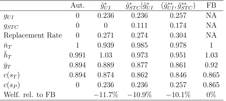
Table 5 presents the results from the three policy experiments for this
parametriza-tion. We maintain the parameters from the original calibration of Table 1 rather than
recalibrating the model. Thus this exercise allows us to compare the welfare effects under
the two parametrizations. The results for experiment ˜gU I∗ show that with UI as the only policy instrument, the optimal net transfer to the unemployed and the associated
replace-ment rate are lower than in experireplace-ment gU I∗ , resulting in a larger welfare loss compared to the first best. This is intuitive given our previous results. Even when financed by
a tax on total hours, UI already imposes an implicit tax on employment which distorts
the composition of labor input. This is exacerbated if UI is financed solely by a tax on
employment. While welfare in all three experiments is lower than in the corresponding
experiment under the original parametrization, the gains of moving from ˜gU I∗ to ˜gST C∗ |g˜∗U I and from ˜g∗ST C|g˜U I∗ to (˜g∗∗U I,˜gST C∗∗ ) are very similar to the corresponding gains in Table 2. The levels of STC are slightly larger relative to UI here. The reason is that STC is similar
to the payroll tax in that it acts as a tax on total hours. Of course it differs from the
eligible for STC. Nonetheless, since under the original parametrization there is already a
tax on total hours even in the absence of STC, the optimal level of STC turns out to be
somewhat lower relative to UI. In this sense, the finding that using the policy instrument
of STC is optimal given parametrization (6) is stronger than the corresponding finding
for parametrization (13).
5.2
Sensitivity Analysis
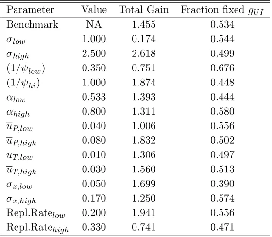
In this section we examine the sensitivity of the welfare results of Section 4.2 to changes
in parameters and targets. Recall that the parametersσ, ψ,α,θ(sP) andσx were chosen
independently, while F and gU I were pinned down by targets for the temporary layoff
rate and the replacement rate. For each parameter in the first group we choose a low and
a high value. Similarly, for each of the two targets we choose a low and a high value. We
vary one parameter or target at a time, and for each deviation from the benchmark we
recalibrate the model and repeat the welfare analysis. The results are shown in Table 6.
In the table, ¯uT and ¯uP denote the targets of the temporary layoff rate and the permanent
layoff rate, respectively. We report two results from the welfare analysis. First, the total
welfare gain is shown in the third column, expressed in consumption equivalent terms
relative to the first best. The fourth column shows what fraction of this gain is achieved
by moving fromg∗U I togST C∗ |g∗
U I, that is, without adjusting the level of UI. The remainder
is then due to moving from gST C∗ |g∗
U I to (g
∗∗
U I, g
∗∗
ST C).
There are several parameters for which variations over a plausible range have little
impact on the results. This includes the curvature of the production function α, the standard deviation of temporary shocks σx, and the temporary layoff rate uT. The
following discussion will focus on the important determinants of the magnitude of welfare
gains.
Naturally, the degree of risk aversion is a key determinant of the magnitude of welfare
gains. Insuring workers hit by uninsured permanent shocks is the only motivation for
using UI in the model. If this motivation is weaker, then the optimal level g∗U I is lower, meaning that the composition of labor inputs is less distorted. This leaves less room for
STC to mitigate the distortions induced by U I.
The Frisch elasticity is also an important determinant of welfare gains: cutting the
elasticity in half to 0.35 cuts the total welfare gain in half. This is intuitive, as the hours
The fraction of workers becoming unemployed due to a permanent shock plays a role
very similar to that of risk aversion. The benefit of UI is to insure this group of workers,
and the magnitude of this benefit is determined by risk aversion in conjunction with the
size of this group.
A higher target for the replacement rate also reduces the total welfare gain. If the
target for the replacement rate is low, then the physical fixed cost F is inferred to be large. This yields a constellation in which the temporary layoff rate is already 0.02 for a replacement rate that is far below optimal. Consequently, the optimal UI rate gU I∗ is associated with a very large temporary layoff rate. In this situation the welfare gains of
STC are large. In contrast, when we target a replacement rate of 33%, then the physical
fixed cost F is inferred to be zero. Thus all temporary layoffs are attributed to UI. Furthermore, the calibrtated level of UI is close to optimal, so the rate of temporary
layoff associated withgU I∗ is also quite low. Thus the scope for STC to reduce the extent of inefficient temporary layoffs is small.
6
Conclusion
In this paper we have studied the welfare effects of short-time compensation (STC) in a
model in which firms have limited access to private insurance and respond to idiosyncratic
profitability shocks by adjusting both employment and hours per worker.
When introduced into an economy with unemployment insurance (UI), STC can affect
welfare through two channels. First, it can mitigate the distortion of the composition of
labor input towards low employment and high hours per worker associated by UI. Second,
STC can directly modify the extent of insurance provided.
We find that the desirability of STC depends on how well firms are already insured
against temporary shocks in the absence of public insurance. If this insurance is good,
introducing STC improves welfare by mitigating the distortions induced by UI.
Further-more, the availability of STC indirectly improves insurance by raising the optimal level
of UI. The effects of STC are quite different when firms are poorly insured against
tem-porary shocks. In this situation firms respond to adverse shocks by combining layoffs
with high hours per worker. The most distressed firms choose to forego STC, with the
consequence that the direct insurance effect of STC is negative, and that STC is unable
to counteract excessive layoffs carried out by these firms.
tem-porary shocks in the absence of public insurance. Our analysis suggests that the extent of
insurance can be identified from the adjustment of labor inputs in response to profitability
References
Burdett, K., and R. Wright. 1989. “Unemployment insurance and short-time
compen-sation: The effects on layoffs, hours per worker, and wages.” Journal of Political
Economy, pp. 1479–1496.
Costain, James S, and Michael Reiter. 2008. “Business cycles, unemployment insurance,
and the calibration of matching models.”Journal of Economic Dynamics and Control
32 (4): 1120–1155.
Feldstein, M. 1976. “Temporary layoffs in the theory of unemployment.” Journal of
Political Economy, pp. 937–957.
Fujita, Shigeru, and Giuseppe Moscarini. 2012. “Recall and Unemployment.” Technical
Report, Mimeo, Yale University, USA.
Hall, R.E. 2009. “Reconciling cyclical movements in the marginal value of time and the
marginal product of labor.” Journal of Political Economy 117 (2): 281–323.
OECD. 2002. “Employment Outlook.”
Topel, Robert H. 1983. “On layoffs and unemployment insurance.” The American
Table 1: Calibration, Temporary Shocks Insured
Value Target
σ 2
ψ 1.43 Frisch elasticity of 0.7
α 0.667
θ(sP) 0.06 unemployment due to permanent shocks 0.06
F(F/y) 0.108(0.121) unemployment due to temporary shocks 0.02
σx 0.1
η 0.40 normalization of average hours to one
H 1 setting normal hours equal to average hours
gU I 0.219 replacement rate 0.25%
gST C 0 no STC in calibration
Table 2: Allocations for Different Policy Configurations, Temporary Shocks Insured
Calibr. Aut. gU I∗ gST C∗ |g∗
U I (g
∗∗
U I, g
∗∗
ST C) FB
gU I 0.219 0 0.248 0.248 0.279 NA
gST C 0 0 0 0.107 0.171 NA
Replacement Rate 0.25 0 0.288 0.292 0.339 NA
¯
nT 0.98 1 0.932 0.981 0.962 1
¯
hT 1 0.991 1.02 0.958 0.929 1.03
¯
yT 0.891 0.894 0.877 0.866 0.839 0.92
c(sT) 0.877 0.894 0.862 0.851 0.822 0.865
c(sP) 0.219 0 0.248 0.248 0.279 0.865
Table 3: Calibration, Temporary Shocks Uninsured
Value Target
σ 2
ψ 1.43 Frisch elasticity of 0.7
α 0.667
θ(sP) 0.06 unemployment due to permanent shocks 0.06
F(F/y) 0.155(0.186) unemployment due to temporary shocks 0.0201
σx 0.1
η 0.4 normalization of average hours to one
H 1 setting normal hours equal to average hours
gU I 0.206 replacement rate 0.25%
gST C 0 no STC in calibration
Table 4: Allocations, Temporary Shocks Uninsured
Calibr. Aut. g∗U I gST C = 12g∗U I FB
gU I 0.206 0 0.219 0.219 NA
gST C 0 0 0 0.11 NA
Replacement Rate 0.25 0 0.269 0.278 NA
¯
nT 0.98 1 0.949 0.953 1
¯
hT 1 0.989 1.01 0.973 1.02
¯
yT 0.836 0.839 0.828 0.802 0.866
¯
cT 0.823 0.839 0.814 0.788 0.814
c(sP) 0.206 0 0.219 0.219 0.814
Welf. rel. to FB −13.2% −12.8% −13.1% 0%
Table 5: Allocations for Alternative Parametrization of Policy, Temporary Shocks Insured
Aut. g˜U I∗ ˜gST C∗ |g˜∗U I (˜gU I∗∗,˜gST C∗∗ ) FB
gU I 0 0.236 0.236 0.257 NA
gST C 0 0 0.111 0.174 NA
Replacement Rate 0 0.271 0.274 0.304 NA
¯
nT 1 0.939 0.985 0.978 1
¯
hT 0.991 1.03 0.973 0.951 1.03
¯
yT 0.894 0.889 0.877 0.861 0.92
c(sT) 0.894 0.874 0.862 0.846 0.865
c(sP) 0 0.236 0.236 0.257 0.865
Table 6: Sensitivity Analysis, Temporary Shocks Insured
Parameter Value Total Gain Fraction fixedgU I
Benchmark NA 1.455 0.534
σlow 1.000 0.174 0.544
σhigh 2.500 2.618 0.499
(1/ψlow) 0.350 0.751 0.676 (1/ψhi) 1.000 1.874 0.448
αlow 0.533 1.393 0.444
αhigh 0.800 1.311 0.580
uP,low 0.040 1.006 0.556
uP,high 0.080 1.832 0.502
uT ,low 0.010 1.306 0.497
uT ,high 0.030 1.560 0.513
σx,low 0.050 1.699 0.390
σx,high 0.170 1.250 0.574
Repl.Ratelow 0.200 1.941 0.556
Figure 1: Subsidy, Hours, and Employment, Temporary Shocks Insured
0.8
1
1.2
1.4
1.6
−0.2
−0.1
0
0.1
0.2
subsidy across
x
x
0.8
1
1.2
1.4
1.6
0.8
1
1.2
1.4
hours across
x
x
0.8
1
1.2
1.4
1.6
0
0.5
1
empl. across
x
x
g
∗ U Ig
∗S T C
|
g
∗U I(
g
∗∗U I
, g
ST C∗∗)
Figure 2: Subsidy, Hours, and Employment, Temporary Shocks Uninsured
0.8
1
1.2
1.4
1.6
−0.11
0
0.11
subsidy across x
x
su
bsi
d
y
0.8
1
1.2
1.4
1.6
−2.2
0
2.2
f
ir
st
be
st
su
bsi
d
y
0.8
1
1.2
1.4
1.6
0.8
1
1.2
1.4
1.6
hours across
x
x
0.8
1
1.2
1.4
1.6
0
0.5
1
empl. across
x
x
g
U I∗g
S T C=
12g
∗U I