PublishedVersionZLB

Nonlinear adventures at the zero lower bound

Jesús Fernández-Villaverde

a

, Grey Gordon

b

, Pablo Guerrón-Quintana

c

,

Juan F. Rubio-Ramírez

d

a

University of Pennsylvania, NBER, and CEPR, United States b

Indiana University, United States

c_{Federal Reserve Bank of Philadelphia, United States} d

Emory University, Federal Reserve Bank of Atlanta, and FEDEA, United States

a r t i c l e i n f o

Article history:

Received 30 September 2014 Received in revised form 19 May 2015

Accepted 21 May 2015 Available online 11 June 2015

JEL classification:

E30 E50 E60

Keywords:

Zero lower bound New Keynesian models Nonlinear solution methods

a b s t r a c t

In this paper, we argue for the importance of explicitly considering nonlinearities in analyzing the behavior of the New Keynesian model with a zero lower bound (ZLB) of the nominal interest rate. To show this, we report how the decision rules and the equilibrium dynamics of the model are substantially affected by the nonlinear features brought about by the ZLB. We also illustrate a tension between the length of a spell at the ZLB and the drop in consumption there.

&2015 Elsevier B.V. All rights reserved.

1. Introduction

This paper argues for the importance of explicitly considering nonlinearities when analyzing the behavior of the New Keynesian model with a zero lower bound (ZLB) on the nominal interest rate. To show this, we first describe how such a model can be efficiently computed using a projection method. Then, we document that

1. The decision rules for variables such as consumption and inflation when the economy is close to or at the ZLB display importantnonlinearities.

2. The distribution of the duration of spells at the ZLB isasymmetric. While the average duration of a spell at the ZLB is 2.06 quarters with a variance of 3.33, spells at the ZLB in our simulation may last up to one decade.

3. The expected duration and the variance of the number of additional periods at the ZLB aretime-varying. The number of expected periods and its variance grows with the number of periods already spent at the ZLB.

4. Repeated shocks over time have highly cumulative nonlinear effects. We can make a spell at the ZLB longer by consecutively hitting the economy with random shocks.

Contents lists available atScienceDirect

journal homepage:www.elsevier.com/locate/jedc

Journal of Economic Dynamics & Control

http://dx.doi.org/10.1016/j.jedc.2015.05.014 0165-1889/&2015 Elsevier B.V. All rights reserved.

5. Themarginal multiplier(the response of the economy to an infinitesimal innovation in government expenditure) and the

average multiplier(the response of the economy to an innovation in government expenditure of sizex) can be quite different.

6. The sizes of fiscal multipliers depend on the combination of shocks that sent the economy to the ZLB. Increases in the variance of the additional number of periods at the ZLB lower the fiscal multipliers.

7. Because of the structure imposed by the household's Euler equation, there is a fundamental trade-off in the properties of the model: one can either generate long spells at the ZLB with catastrophic drops in consumption or one can generate short spells at the ZLB with moderate drops in consumption. But one cannot generate long spells at the ZLB with moderate drops in consumption, which we have observed in recent U.S. data.

8. One can, however, get arbitrarily long spells at the ZLB with moderate drops in consumption if one introduces a wedge in the household's Euler equation.

Results 1_–3 show that the dynamics of the model are often poorly approximated by a linear solution. Result 4 implies that consecutive shocks do not add up, as they would in a linear world. Instead, nonlinearities make their effect grow exponentially. This is important, for example, for the design of econometric tools to study the effects of the ZLB. Results 5 and 6 demonstrate that the nonlinearities matter for the evaluation of fiscal policy. Results 7 and 8 offer relevant insights into how to improve the model's performance in matching the recent empirical evidence and suggest avenues for future research.

Our investigation is motivated by the U.S. and Eurozone experience of (nearly) zero short-term nominal interest rates after 2008. This experience has rekindled interest in the role of the ZLB for issues such as monetary policy (Eggertsson and Woodford, 2003) and fiscal policy (Christiano et al., 2011). However, the analysis of the ZLB is complicated by the essential nonlinearity in the function that determines the nominal interest rates. This nonlinearity means that, by construction, both linearization techniques and higher-order perturbations cannot handle the ZLB.

The literature has tried to get around this problem using different approaches. We highlight three of the most influential.

Eggertsson and Woodford (2003)log-linearize the equilibrium relations except for the ZLB constraint, which is retained in its exact form. They then solve the corresponding system of linear expectational difference equations with the linear inequality constraint.Christiano et al. (2011)linearize the two models they use: a simple model without capital and a model with capital.

Braun and Körber (2012)employ a variant of extended shooting, which solves the model forward for an exogenously fixed number of periods assuming that, in these periods, shocks are set to zero. Most researchers in the area have followed some variation of these approaches (in the interest of space, we skip a more thorough review of that literature).

Although a step forward, the existing solutions may have unexpected implications. First is linearizing equilibrium conditions may hide nonlinear interactions between the ZLB and the decision rules of the agents. This point is demonstrated byBraun et al. (2012), who show how labor supply can fall in the log-linear approximation but rise in the exact nonlinear solution. Second, linear approximations provide a poor description of the economy during deep recessions such as the one in 2007–2009. Third, dynamics driven by exogenous variables that follow simple Markov chains with absorbing states or have deterministic paths imply that the durations of spells at the ZLB have simple expectations and variances. When we solve the model nonlinearly, however, these expectations and variances change substantially over time. This is key because the distribution of future events has material consequences for important quantities such as the size of the fiscal multiplier. We address these nonlinear interactions and the time-varying distributions of future events by computing a nonlinear New Keynesian model with a ZLB. We incorporate monetary and fiscal policy and four different shocks. The agents in the model have the right expectations about the probability of hitting the ZLB. We employ the Smolyak collocation method laid out inKrueger et al. (2011)and applied byWinschel and Krätzig (2010)to solve for the nonlinear equilibrium functions for consumption, inflation, and the one auxiliary variable. The Smolyak collocation method significantly reduces the burden of the curse of dimensionality. Once we have the three nonlinear equilibrium functions, we exploit the rest of the equilibrium conditions of the model to solve for the remaining variables. Our approach computes the Taylor rule with a ZLB indirectly, allowing the kink at zero to be fully respected and obviating the need to approximate a non-differentiable function.

After we circulated our first draft in 2012, several papers have further explored the nonlinear dynamics of New Keynesian models with a ZLB (also, a few years ago, Wolman (1998), solved a simpler sticky prices model using finite elements). Among those,Judd et al. (2012)merge stochastic simulation and projection approaches that share some similarities with our algorithm. The main thrust of the paper is computational, and they solve the New Keynesian model as a brief illustration.Nakata (2013)uses a time iteration algorithm, but he has only one state variable.Aruoba and Schorfheide (2012)

explore the dynamics created by the presence of multiple equilibria.Gavin et al. (2014)analyze a model similar to ours, but with Rotemberg pricing.Richter and Throckmorton (2015)analyze convergence of models with a ZLB. They find that their solution method does not converge if the ZLB is hit too frequently or if the expected duration at the ZLB is too long.

The rest of this paper is organized as follows. Insection 2, we present a baseline New Keynesian model and we calibrate it to the U.S. economy. Insection 3, we show how we compute the model nonlinearly. InSections 4and5, we present our quantitative findings. Section 6 illustrates the trade-offs between the length of the spell at the ZLB and drops in consumption imposed by the household's Euler equation, and it explains how to improve upon this trade-off.Section 7

concludes. A technical appendix offers further details.

2. The model

Our investigation is built around a baseline New Keynesian model, which is often used to discuss the ZLB. In this economy, a representative household consumes, saves, and supplies labor. Output is assembled by a final good producer from a continuum of intermediate goods manufactured by monopolistic competitors. The intermediate good producers rent labor from the household. Also, these intermediate good producers change prices following a Calvo rule. A government fixes the one-period nominal interest rate, sets taxes, and consumes. All the agents have rational expectations. There are four shocks: to the time discount factor, to technology, to monetary policy, and to fiscal policy.

2.1. Household

A representative household maximizes a lifetime utility function separable in consumptionctand hours workedlt;

E0

X1

t¼0

∏t

i¼0

β

i

!

logct

ψ

l

1þϑ

t 1þ

ϑ

( )

:

The discount factor

β

tfluctuates around its mean

β

with a persistence

ρ

b, innovations

ε

b;t, and a law of motion

β

t¼

β

1ρb

β

ρb

t1expð

σ

b

ε

b;tÞ where

ε

b;tNð0;1Þand

β

0¼

β

:

The household trades Arrow securities (which, since they are in zero net supply, we do not discuss further) and a nominal government bondbtthat pays a nominal gross interest rate ofRt:Then, given a pricept of the final good, the household's budget constraint is

ctþ

btþ1

pt

¼wtltþRt1

bt

pt

þTtþ

ϝ

t

wherewtis the real wage,Ttis a lump-sum transfer, and

ϝ

tare the profits of the firms in the economy. The first-order conditions of this problem are

1

ct

¼Et

β

tþ1 1

ctþ1

Rt

Π

tþ1

ψ

lϑtct¼wt;

where

Π

tþ1¼ptþ1=ptis inflation.

2.2. The final good producer

The final goodytis produced using intermediate goodsyitand the technology

yt¼

Z 1

0

yð_itε1Þ=εdi !ε=ðε1Þ

ð1Þ

where

ε

is the elasticity of substitution. The final good producer maximizes profits subject to the production function (1)

taking as givenptand all intermediate goods pricespit. Then, we have thatpt¼

R1 0p

1ε

it di

1=ð1εÞ

.

2.3. Intermediate good producers

Each intermediate firm produces differentiated goods usingyit¼Atlit, wherelitis the amount of labor rented by the firm. ProductivityAtfollowsAt¼A1ρaAρta1expð

σ

a

ε

a;tÞ, whereAis a constant and

ε

a;tNð0;1Þ.

The monopolistic firms set prices á la Calvo. In each period, a fraction 1

θ

of intermediate good producers reoptimize their prices topn

t¼pit (the reset price is common across all firms that update their prices). All other firms keep their old prices. The solution forpn

t has a recursive structure in two auxiliary variablesx1;tandx2;tthat satisfy

ε

x1;t¼ ð

ε

1Þx2;tand have laws of motion

x1;t¼ 1

ct

wt

At

and

x2;t¼ 1

ct

Π

n

tytþ

θ

Et

β

tþ1

Π

ε

1

tþ1

Π

n t

Π

n

tþ1

x2;tþ1¼

Π

nt 1

ct

ytþ

θ

Et

β

tþ1

Π

ε1

tþ1

Π

n

tþ1

x2;tþ1

!

where

Π

nt¼pnt=pt and

Π

t¼pt=pt1. Also, inflation satisfies 1¼

θΠ

ε

1

t þð1

θ

Þð

Π

ntÞ

1ε_.

2.4. The government

The government sets the nominal interest rate according toRt¼max½Zt;1where

Zt¼R1ρrRρtr1

Π

t

Π

ϕπ _y

t

y ϕy

" #1ρr

mt:

The variable

Π

is the target level of inflation andR¼

Π

=

β

the target nominal gross return of bonds. The term mt is a monetary policy shock that followsmt¼exp

σ

m

ε

m;t

with

ε

m;tNð0;1Þ. This policy rule is the maximum of two terms. The first term,Zt, is a conventional Taylor rule. The second term is the ZLB:Rtcannot be lower than 1.

Beyond the open market operations, the lump-sum transfers also finance government expendituresgt¼sg;tyt with

sg;t¼s

1ρg

g sρgg;t1expð

σ

g

ε

g;tÞwhere

ε

g;tNð0;1Þ: ð2Þ Because of Ricardian irrelevance, the timing of these transfers is irrelevant, so we setbt¼0.1

2.5. Aggregation

Aggregate demand is given by yt¼ctþgt. By well-known arguments, aggregate supply is yt¼ ðAt=vtÞlt where

vt¼

R1 0 ðpit=ptÞ

ε_{diis the aggregate loss of efficiency induced by the dispersion ofp}

it. By the properties of Calvo pricing,

vt¼

θΠ

εtvt1þð1

θ

Þð

Π

ntÞ _ε

.

2.6. Equilibrium

The definition of equilibrium in this model is standard. This equilibrium is given by the sequence

fyt;ct;lt;x1;t;x2;t;wt;

Π

t;

Π

tn;vt;Rt;Zt;

β

t;At;mt;gt;sg;tg 1

t¼0determined by

the first-order conditions of the household

1

ct¼Et

β

tþ1

ctþ1

Rt

Π

tþ1

ψ

lϑ_tct¼wt

profit maximization

ε

x1;t¼ð

ε

1Þx2;t

x1;t¼ 1

ct

wt

At

ytþ

θ

Et

β

tþ1

Π

εtþ1x1;tþ1

x2;t¼

Π

nt 1

ct

ytþ

θ

Et

β

tþ1

Π

ε1

tþ1

Π

n

tþ1

x2;tþ1

!

government policy

Rt¼max½Zt;1

Zt¼R1ρrRρtr1

Π

t

Π

ϕπ _y

t

y ϕy

" #1_ρr

mt

gt¼sg;tyt

1

inflation evolution and price dispersion

1¼

θΠ

ε1

t þð1

θ

Þð

Π

ntÞ1 _ε

vt¼

θΠ

εtvt1þð1

θ

Þð

Π

ntÞ _ε

market clearing

yt¼ctþgt

yt¼

At

vt

lt

and the stochastic processes

β

t¼

β

1ρb

β

ρb

t1expð

σ

b

ε

b;tÞ

At¼A1ρaAtρa1expð

σ

a

ε

a;tÞ

mt¼expð

σ

m

ε

m;tÞ

sg;t¼s

1ρg

g sρg;gt1expð

σ

g

ε

g;tÞ:

Models with a Taylor rule display, in general, multiple steady states (Benhabib et al., 2001). On several occasions, we will refer to the steady state of the model with positive inflation (although our solution method does not use that steady state). We use the vectorfy;c;l;x1;x2;w;

Π

;

Π

n;v;R;Z;

β

;A;m;g;sggto stack the variables in such a steady state, where we have eliminated subindexes to denote a steady-state value. See the appendix for details.

2.7. Calibration

We calibrate the model to standard choices. We set

β

¼0:994 to match an average annual real interest rate of roughly 2.5 percent,

ϑ

¼1 to deliver a Frisch elasticity of 1 (in the range of the numbers reported when we consider both the intensive and the extensive margin of labor supply), and

ψ

¼1;a normalization of the hours worked that is nearly irrelevant for our results. As is common in the New Keynesian literature, we set

θ

¼0:75 and

ε

¼6, which implies a mean duration of prices of 4 quarters and an average markup of 20 percent (Christiano et al., 2005;Eichenbaum and Fisher, 2007).

The parameters in the Taylor rule are conventional:

ϕ

_π¼1_:5,

ϕ

y¼0:25,

Π

¼1:005, and, to save on the dimensionality of the problem,

ρ

r¼0 (this is also the case inChristiano et al., 2011). ThenRt¼maxðR=

Π

ϕπyϕyÞ

Π

ϕtπy

ϕy t mt;1

h i

. For fiscal policy,

sg¼0:2 so that government expenditures on average account for 20 percent of output, which is close to the average of government consumption in the U.S.

With respect to the shocks, we set

ρ

b¼0:8 and

σ

b¼0:0025. Thus, the preference shock has a half-life of roughly 3 quarters and an unconditional standard deviation of 0.42 percent. With these values, our economy hits the ZLB with a frequency consistent with values previously reported (seeSection 5below for details). For technology, we setA¼1,

ρ

a¼0:9; and

σ

a¼0:0025. These numbers reflect the lower volatility of productivity in the last two decades. Following Guerró n-Quintana (2010), we pick

σ

m¼0:0025. For the government expenditure shock, we have somewhat smaller values than Christiano et al. (2011) by setting

ρ

g¼0:8 and

σ

g¼0:0025. This last value is half of that estimated in Justiniano and Primiceri (2008). Those numbers avoid the numerical problems associated with very persistent fiscal shocks when we hit the economy with a large fiscal expansion. In sensitivity analysis reported in the technical analysis we argue that this lower persistence is not terribly important for the points we want to make in this paper.

3. Solution of the model

Given the previous calibration, our model has five state variables: price dispersion, vt1; the time-varying discount factor,

β

t; productivity,At; the monetary shock,mt; and the government expenditure share,sg;t. Then, we define the vector of state variables:

St¼ ðS1;t;S2;t;S3;t;S4;t;S5;tÞ ¼ ðvt1;

β

t;At;mt;sg;tÞ;

with one endogenous state variable and four exogenous ones. For convenience, we also define the vector evaluated at the steady state with positive inflation asSss¼ ðv;

β

;1;1;sgÞ.

is interpolated at the grid points. Although the algorithm is described in detail in the appendix, its basic structure is as follows.

The equilibrium functions forct,

Π

t, andx1;tcan be written as functions of the states as

ct¼f1ðStÞ

Π

t¼f2ðStÞ

x1;t¼f

3

ðS^tÞ

wheref¼ ðf1;f2;f3Þandfi:R5_{-RforiAf1;2;3g. If we had access tof, we could find the values of the remaining endogenous} variables using the equilibrium conditions. Sincefis unknown, we approximatect,

Π

t, andx1;t as

ct¼bf

1

ðStÞ

Π

t¼bf

2

ðStÞ

x1;t¼bf

3

ðStÞ

wherebf¼ ðb_f1_;b_f2_;b_f3_{Þare polynomials.}

To computebf, we first define a hypercube for the state variables (we extrapolate when we need to move outside the hypercube in the simulations) and rely on Smolyak's algorithm to obtain collocation points (grid points) within the hypercube. We guess the values ofbf at those collocation points, which implicitly definebf over the entire state space. Then, treatingbf as the true timetþ1 functions, we exploit the equilibrium conditions to back out the values ofct;

Π

t, andx1;tat the collocation points and check that those values coincide with the ones implied bybf. If not, we update our guess until convergence. In our application, we use polynomials of up to degree 4 (and for an accuracy check in section 10, up to degree 8).

Once we have foundbf, from the equilibrium conditions we get an expression for the second auxiliary variable,

x2;t¼

ε

ε

1x1;t; output,

yt¼ctþgt¼ctþsgsg;tyt¼ 1 1sgsg;t

ct;

and for reset prices (relative topt),

Π

n

t¼

1

θΠ

ε1

t 1

θ

!1=ð1_εÞ :

Then, we get the evolution of price dispersion,vt¼

θΠ

εtvt1þð1

θ

Þð

Π

ntÞ

ε_{, labor,l}

t¼ ðvt=AtÞyt, wages,wt¼

ψ

lϑtct, and the interest rate:

Rt¼max

R

Π

ϕπ_yϕy

Π

ϕπ t y

ϕy t mt;1

" #

:

Thus, with this procedure, we get a set of functions ht¼hðStÞ for the additional variables in our model

htAfyt;lt;x2;t;wt;

Π

nt;vt;Rtg.

A key advantage of our procedure is that we solve nonlinearly for ct,

Π

t, and x1;t and later for the other variables exploiting the remaining equilibrium conditions. Hence, conditional onct,

Π

t, andx1;t, our method deals with the kink ofRt at 1 without any approximation:Rtcomes from a direct application of the Taylor rule. Also, the functions forct,

Π

t, andx1;t are derived from equations that involve expectations, which smooth out any possible kinks created by the ZLB.

In the technical appendix, we compute (log10) Euler equation errors for a range of values of the state space. The errors,

even in the areas where the ZLB is likely to bind, are between 3 and5. That is roughly the same (or perhaps slightly better) than for a log-linearized version of the model without the ZLB. We also compute average, median, and maximum residuals over the simulation of 300,000 periods that we report in Section 5(we also plot the histogram of the Euler equation errors). The mean of the Euler equation error is 3.26, the median is 3.17, and the maximum error is 1.65. However, in such a long simulation, the maximum error may be an extreme event. If we trim the worst 0.1 percent of errors, we find 99.9 percent of the errors are less than a very solid2.21 ($1 for each $ 162 spent).

4. Comparison of decision rules

and continue). In the interest of space, we focus on the decision rules for consumption and inflation and the effect of the discount factor shock.

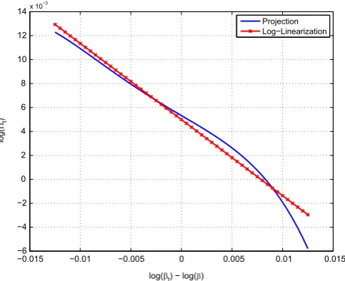
First,Fig. 1plots our nonlinear decision rule for consumption and the log-linear approximation

logctlogc¼

α

1ðlogvt1logvÞþ

α

2ðlog

β

tlog

β

Þþ

α

3logAtþ

α

4logmtþ

α

5ðlogsg;tlogsgÞ:

along the log

β

t-axis, while we keep the other state variables at their steady-state values. The decision rule has a negative slope since a higher discount factor induces the household to save more, which lowers the real interest rate. Hence, if sufficiently large and positive innovations buffet the discount factor, the economy may be pushed to the ZLB. We observe this urgency to save more in the nonlinear policy. Consumption plunges for shocks that push the discount factor 0.7 percent or more above

β

. This is not a surprise. We calibrated

β

to be 0.994. Then, when the discount factor increases 0.6 percent (0.006 in our graph),

β

tbecomes greater

than 1 and future consumption yields more utility than current expenditure. Our projection method responds to that feature of the model. The projection method does not deliver a decision rule that is globally concave. Since we have price rigidities, there is no reason to expect global concavity. In contrast, the log-linear approximation, since it is built around

β

t¼

β

, predicts a stable decline in consumption. This difference becomes stronger as

β

tmoves into higher values. At the same time, the two policies almost

coincide for values of the discount factor close to or below

β

, where the log-linear approximation is valid (although there is also a small difference in levels due to precautionary behavior, which is not captured by the log-linear approximation).

−0.015 −0.01 −0.005 0 0.005 0.01 0.015 −0.225

−0.22 −0.215 −0.21 −0.205 −0.2 −0.195 −0.19

log(βt) − log(β)

log(C

t

)

Projection Log−Linearization

Fig. 1. Log-linear versus nonlinear decision rules for consumption.

−0.015 −0.01 −0.005 0 0.005 0.01 0.015 −6

−4 −2 0 2 4 6 8 10 12 14

log(

Πt

)

Projection Log−Linearization

log(βt) − log(β)

The policy function for inflation (Fig. 2) confirms the previous pattern. As the discount factor becomes bigger, there is less aggregate demand today, and this pushes inflation down as those firms that reset their prices do not raise them as much as they would otherwise. In the nonlinear solution, this phenomenon of contraction-deflation becomes more acute as

β

increases and the economy moves toward the ZLB.

In conclusion, nonlinearities matter when we talk about the decision rules under the ZLB. The consequences of this difference will be even clearer in the next section.

5. Simulation results

The second step in our illustration of the importance of nonlinearities in a New Keynesian model with the ZLB is to report some simulation results.

5.1. Probability of being at the ZLB

Since, in our model, the entry and exit from the ZLB is endogenous, we start by deriving the probability that the economy is at the ZLB in any particular period. Thus, we compute

PrðfRt¼1gÞ ¼

Z

If1g½RðStÞ

μ

ðStÞdSt ð3Þ

for alltZ1, whereIB½fðxÞ:Rn-f0;1gis the indicator function of a setBRk andf:Rn-Rk, defined as

IB½fðxÞ ¼

1 iffðxÞAB

0 iffðxÞ2=B (

for anyn, and where

μ

ðStÞis the unconditional distribution of the states of the economy. We further defineIB½xasIB½

ι

ðxÞ, where

ι

is the identity map.

We simulate the model forT¼300;000 periods starting atSsswith our solution fromSection 3. We define the sequence of simulated states asfSi;ssgTi¼1, whereSi;ssis the value of the state vector in periodiof the simulation when the initial condition isSss.2Using this sequence, we follow Santos and Peralta-Alva (2005) to approximate Eq.(3)by

PrðfRt¼1gÞCcPrðfRt¼1gÞ ¼

PT

i¼1If1g½RðSi;ssÞ

T : ð4Þ

As expected from the calibration, our economy is at the ZLB during 5.53 percent of quarters, or approximately 1 out of each 18 quarters. This percentage is close to the findings ofReifschneider and Williams (1999)andChung et al. (2010)using the FRB/US model.

Also, since the probability of being at the ZLB is not independent of the history of states, we calculate the probability of being for at least one extra period at the ZLB conditional on having been at the ZLB for exactlysperiods as

PrðfRt¼1gjfRt1¼1;…;Rts¼1;Rts141gÞ

¼ Z

If1g½RðStÞ

μ

ðStjfRt1¼1;…;Rts¼1;Rts141gÞdSt

for alltZ3 andt2ZsZ1.

If we let Rt1;s¼ fRt1¼1;…;Rts¼1;Rts141g for all tZ3 and t2ZsZ1, then the above expression can be rewritten as

PrðfRt¼1gjRt1;sÞ ¼

Z

If1g½RðStÞ

μ

ðStjRt1;sÞdSt ð5Þ

for alltZ3 andt2ZsZ1 and where

μ

ðStjRt1;sÞis the distribution of the states conditional onRt1;s. ForsZ1, letfSiks;ssg

Ms

ks¼1be theMselements of the sequencefSi;ssg T

i¼1such thatRðSiks1;ssÞ ¼1,…,RðSikss;ssÞ ¼1, and

RðSikss1;ssÞ41 for allksAf1;…;Msg. We then approximate(5)by

Pr fRt¼1gjRt1;s

CcPr fRt¼1gjRt1;s

¼ X

Ms

ks¼1

If1g½RðSiks;ssÞ

Ms

ð6Þ

forMs40. WhenMsis 0, we saycPrðfRt¼1gjRt1;sÞ ¼0.

Table 1reports the values of Eq.(6)forsfrom 1 to 10. The probability of being at the ZLB for at least one extra period increases from 44 percent conditional on having been at the ZLB for 1 period to 65 percent for 5 periods and fluctuates

2

thereafter.3_{That is, during the first year of a spell at the ZLB, the longer we have been at the ZLB, the more likely it is we will} stay there next period. The intuition is simple: if we have been at the ZLB for, say, 4 quarters, it is because the economy has suffered a string of bad shocks. Thus, the economy will linger longer on average around the state values that led to the ZLB in the first place. The probabilities inTable 1point out a key feature of our model that will resurface in the next subsections: the expectation and variance of the time remaining at the ZLB are time-varying.

5.2. How long are the spells at the ZLB?

To determine the length of the spells at the ZLB, we compute the expected number of consecutive periods that the economy will be at the ZLB right after entering it. Formally

EðTtjRt1;1Þ ¼

X1

j¼1

ðjPrðfTt¼jgjRt1;1ÞÞ

¼X

1

j¼1

j Z

Ifjg½Tt

μ

ðSt;Stþ1;…jRt1;1ÞdStdStþ1…

ð7Þ

for alltZ3, whereRt1;1describes the event“entering the ZLB,”

μ

ðSt;Stþ1;…jRt1;1Þis the distribution of the sequence of future states conditional on_Rt1;s, andTt¼TðSt;Stþ1;…Þ ¼minf

ω

:

ω

Af1;2;…gandRtþω1¼RðStþω1Þ41gfor alltZ3 is the first period outside the ZLB as a function of the future path of state variables. IfTt¼1, thenRt41 for that path. In the same way, ifTt¼2, thenRt¼1 andRtþ141 for that path of state variables.

To approximate the expectation in(7), take Sik1;ss

n oM1

k1¼1

and calculate

E TtjRt1;1

Cb_{E Tt}jRt1;1

¼X

T2

j¼1

j X

M1

k1¼1

Ifjg T Sb ik1þ1;ss;…;ST;ss

h i

M1

0 @

1 A 0

@

1

A ð8Þ

where we approximate the probability

PrðfTt¼jgjRt1;1Þ ¼

Z

Ifjg½Tt

μ

ðSt;Stþ1;…jRt1;1ÞdStdStþ1…

for alltZ3 andT2ZjZ1, by

Pr fTt¼jgjRt1;1

Cc_{Pr T}bt¼j

n o

jRt1;1

¼ X

M1

k1¼1

Ifjg T Sb ik1;ss;…;ST;ss

h i

M1

whereTbt¼TbðSt;…;STÞ ¼minf

ω

:

ω

Af1;2;…;Ttþ1gand Rtþ_ω1¼RðStþ_ω1Þ41gfor alltZ3. The expression(8)equals 2.06 quarters in our simulation. That is, on average, we are at the ZLB for slightly more than half a year after entering it. Note that, given our simulation ofTperiods, we can be at the ZLB at mostT2 (we need a period before entry and one period of exit of the ZLB). Also, we approximateT Sik₁;ss;Sik₁þ1;ss;…

byT Sb ik₁;ss;…;ST;ss

. But this approximation has no effect as long asRðST;ssÞ41.

We can also compute the variance of the number of consecutive periods at the ZLB right after entering it:

VarðTtjRt1;1Þ ¼

X1

j¼1

ððjEðTtjRt1;1Þ2PrðfTt¼jgjRt1;1ÞÞ

¼X

1

j¼1

ðjEðTtjRt1;1Þ2

Z

Ifjg½Tt

μ

ðSt;Stþ1;…jRt1;1ÞdStdStþ1…

Table 1

Probability of being at the ZLB for at least one extra period.

1 2 3 4 5 6 7 8 9 10

c

PrðfRt¼1gjRt1;sÞ(%) 44 54 60 62 65 60 65 67 65 60

3

for alltZ3, which we approximate by

VarTtjRt1;1

CVard TtjRt1;1

¼ X

T2

j¼1

jb_EðTtjRt1;1Þ

2 XM1

k1¼1

Ifjg T Sb ik₁;ss;…;ST;ss

h i M1 0 @ 1 A_:

By applying the previous steps, we find that the variance is 3.33 quarters. Since the number of consecutive periods at the ZLB is bounded below by 1 quarter (one period in our model), a variance of 3.33 (standard deviation of 1.8 quarters) denotes a quite asymmetric distribution with a long right tail. We revisit this issue below.

Now, we would like to see how the conditional expectations and variance depend on the number of periods already at the ZLB. First, we calculate the expected number of additional periods at the ZLB conditional on having already been at the ZLB forsperiods:

EðTt1∣Rt1;sÞ ¼

X1

j¼1

ððj1ÞPrðfTt¼jg∣Rt1;sÞÞ

¼X

1

j¼1

ðj1Þ Z

Ifjg½Tt

μ

ðSt;Stþ1;…∣Rt1;sÞdStdStþ1…

for alltZ3 andt2ZsZ1, where we are subtracting 1 fromTt because we are calculating the number of additional periods at the ZLB. This expression can be approximated by

b

E Tt1∣Rt1;s

¼ X

Ts1

j¼1

j1

ð Þ X

Ms

ks¼1

Ifjg TbðSiks;ss;…;ST;ssÞ

h i Ms 0 @ 1 A_:

We build the analogous object for the conditional variance:

VarðTt1∣Rt1;sÞ ¼

X1

j¼1

ðjEðTts∣Rt1;sÞÞ2PrðfTt¼jg∣Rt1;sÞ

¼X

1

j¼1

ðjEðTtjRt1;sÞÞ2

Z

Ifjg½Tt

μ

ðSt;Stþ1;…∣Rt1;sÞdStdStþ1…

:

approximated by

d

Var TtjRt1;s

¼ X

Ts1

j¼1

jb_EðTtjRt1;sÞ

2 XMs

ks¼1

Ifjg TbðSiks;ss;…;ST;ssÞ

h i Ms 0 @ 1 A_:

Recall that, given our simulation ofTperiods, we can be at the ZLB at mostTs1 additional periods (we needsperiods before entry and one period of exit of the ZLB).

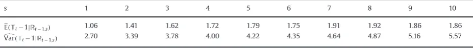
These two statistics are reported inTable 2. The expected number of additional periods increases with the number of periods already at the ZLB (at least until 8 quarters) and the variance grows monotonically, from 2.70 to 5.57. Hence, the agents have more uncertainty forecasting the periods remaining at the ZLB as the time at the ZLB accumulates.

The results inTable 2reflect how the distribution of additional periods at the ZLB is time-varying. This is an important difference of our paper with respect to the literature. Previous papers have considered two cases. In the first one, there is an exogenous variable that switches in every period with some constant probability; the typical change is the discount factor going from low to high. Once the variable has switched, there is a perfect foresight path that exists from the ZLB (see, for instance,Eggertsson and Woodford, 2003). Although this path may depend on how long the economy has been at the ZLB, there is no uncertainty left once the variable has switched. In the second case, researchers have looked at models with perfect foresight (see, for example,Sections 4and5ofChristiano et al., 2011). Even if fiscal policy influences how long we are at the ZLB, there is no uncertainty with respect to events, and the variance is degenerate.

The number of additional periods at the ZLB and the beliefs that agents have about them will play a key role later when we talk about the fiscal multiplier. The multiplier will depend on the uncertainty regarding how many more periods the economy will be at the ZLB. Having more uncertainty will, in general, raise the multiplier. However, the result cannot be ascertained in general because of the skewness of the distribution. By construction, we cannot have fewer than zero additional periods at the ZLB. Thus, if the expectation is, for instance, 1.79 quarters and the variance is 4.22 (columns¼5 inTable 2), we must have a large right tail and a

Table 2

Number of additional periods at the ZLB.

s 1 2 3 4 5 6 7 8 9 10

b

EðTt1jRt1;sÞ 1.06 1.41 1.62 1.72 1.79 1.75 1.91 1.92 1.86 1.86 d

concentrated mass on the (truncated) left tail. A higher variance can be caused by movements in different parts of this asymmetric distribution and, thus, has complex effects on the fiscal multiplier (as we discuss more inSection 5.7).

5.3. What shocks take us to the ZLB?

We would like to know whether a shock of a given size increases or decreases the probability of hitting the ZLB in the nextIperiods. More concretely, we would like to compute

Prð[I

i¼1fRtþi¼1g∣fSj;t¼AjgÞ ¼

Z

maxfIf1g½RðStþ1Þ;…;If1g½RðStþIÞg

μ

ðStþ1;…;StþI∣fSj;t¼AjgÞdStþ1…dStþI ð9Þ

forAjARand whereSj;tis thejth element ofSt. We perform this analysis only for the exogenous state variables, that is

j_Af2_;…;5g.

To approximate(9), we simulate the modelN¼10,000 times forIperiods starting atSssfor all states, except for thejth element ofSt, which we start atAj. For each simulationnAf1;…;Ng, we call theI-periods-long sequence of statesfSA_nj_;i;ssg

I i¼1. Then, we setI¼10 and approximate the probability by

c

Pr [I

i¼1fRtþi¼1gjfSj;t¼Ajg

¼ X

N

n¼1

max If1g R SA_nj_;1;ss

h i

;…;If1g R SA_n;j_I;ss

h i

N :

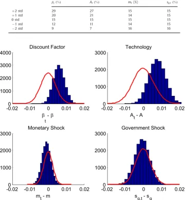
Table 3 reports these probabilities when the initial exogenous states are set, one at a time (corresponding to each column), to 0, 71, and 72 standard deviation innovations away from their steady state. In other words,

Aj¼Sj;ss7f0;1;2g

σ

j for the discount factor, technology, monetary policy, and government expenditure. The third row (labeled 0 std) shows a baseline scenario in which all the exogenous states are set at their steady-state values. In this baseline, the probability of getting to the ZLB in the next two and a half years is 15 percent (all the entries in the row are equal, since we are describing the same event). When we have a one-standard-deviation positive innovation to the discount factor, that probability goes up to 20 percent, and to 29 percent when we have a two standard deviations innovation.

When

β

tis higher than

β

, the household is more patient and the interest rate that clears the good market is low. Hence, it

is easy for the economy to be pushed into the ZLB. The reverse results occur when the innovation is negative: the probability of entering into a ZLB falls to 12 percent (one standard deviation) or 9 percent (two standard deviations). Positive productivity shocks also raise the probability of being at the ZLB. There are two mechanisms at work here. First, higher productivity means lower marginal costs and lower inflation. Since the monetary authority responds to lower inflation by lowering the nominal interest rate even more (

ϕ

_π¼1_:5), this puts the economy closer to the ZLB. Second, when productivity is high, a lower real interest rate induces households to consume more and clear the markets. This lower real interest rate translates, through the working of the Taylor rule, into a lower nominal interest rate.4_{Finally, monetary and fiscal policy} shocks have a volatility that is too small to change much the probability of hitting the ZLB.

Complementary information is the distribution of states conditional on being at the ZLB:

μ

ðStjfRt¼1gÞ: ð10Þ

LetfSik;ssg M

k¼1be theMelements subsequence of the sequencefSi;ssgTi¼1such thatRðSik;ssÞ ¼1 for allkAf1;…;Mg. Then, we

approximate(10)by

μ

ðfStAAgjfRt¼1gÞC

PM

k¼1IAðSik;ssÞ

M ð11Þ

for any setAR5_{. SinceS}

tAR5, it is hard to represent Eq.(11)graphically. Instead, inFig. 3we represent the four individual marginal distributions

μ

fSj;tAAjgjfRt¼1g

C

PM

k¼1IAiðSj;ik;ssÞ

M

for any setAjR, whereSj;tis thejth element ofStandSj;ik;ssis thejth element ofSik;ss(we drop the distribution forvt1,

since it has a less clear interpretation). To facilitate comparison, the states are expressed as deviations from their average values and we plot, with the red continuous line, the unconditional distribution of the state.

InFig. 3we see a pattern similar to the one inTable 3: high discount factors and high productivity are associated with the ZLB while the fiscal and monetary shocks are nearly uncorrelated. The same information appears inTable 4, where we report the mean and the standard deviation of the four exogenous variables, unconditionally and conditional on being at the ZLB. The ZLB is associated with high discount factors and high productivities, but it is not correlated with either monetary or

4

fiscal policy. In the appendix, we also report the bivariate conditional distributions of the exogenous states:

μ

ððSi;t;Sj;tÞ∣fRt¼1gÞ ð12Þ

whereSj;tis thejth element ofSt andi;jAf2;…;5g.

-0.02

0

-0.01

0

0.01

0.02

1000

2000

3000

4000

t

β β

-

Discount Factor

-0.02

0

-0.01

0

0.01

0.02

1000

2000

3000

A

t

- A

Technology

-0.02

0

-0.01

0

0.01

0.02

1000

2000

3000

m

t

- m

Monetary Shock

-0.02

0

-0.01

0

0.01

0.02

1000

2000

3000

s

g,t

- s

g

Government Shock

Fig. 3.Distribution of exogenous states, unconditional and conditional on being at the ZLB. (For interpretation of the references to color in this figure caption, the reader is referred to the web version of this paper.)

Table 4

Unconditional and conditional moments of (log of) exogenous states.

Mean (%) Std (%)

log of β A m sg β A m sg

Unconditional 0.00 0.00 0.00 0.00 0.41 0.58 0.25 0.42

At ZLB 0.60 0.78 0.10 0.07 0.32 0.47 0.25 0.42

Table 3 c Prð[I

i¼1fRtþi¼1gjfSj;t¼AjgÞ.

βtð%Þ Atð%Þ mt(%) sg;tð%Þ

þ2 std 29 27 15 15

þ1 std 20 21 14 15

0 std 15 15 15 15

1 std 12 11 14 15

5.4. Nonlinear accumulation of shocks

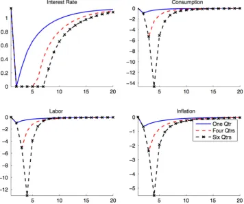
We now investigate a key feature of the dynamics of the model: the accumulation of random shocks over time has highly nonlinear effects. More precisely, we shock the economy—which is at its steady state—with unanticipated increases in the discount factor (the size of each shock is always 0.0096). We do this in three different cases (the corresponding IRFs are plotted inFig. 4). In the first case, there is only one shock at time 1, which sends the economy to the ZLB for exactly one period (blue line). The second experiment has the economy buffeted by unanticipated discount factor shocks at periods 1 and 2 (discontinuous red line). The size of the shocks is such that the economy remains at the ZLB for four periods. Finally, when we hit the economy in periods 1 to 3 (crossed black line) with unanticipated discount factor shocks, the interest rate is at zero for six periods.

The IRFs display the expected pattern: after the increase in the discount factor, the nominal interest rate, consumption, hours, and inflation go down at impact and later recover back to their original values. What is interesting is how the IRFs reveal the intrinsically nonlinear nature of the ZLB. After the first negative shock, consumption falls 0.93 percent (the first period is the same for all three cases). However, after the second shock arrives, output falls to 5.27 percent below its steady-state value. In the absence of this second shock, output would have recovered to0.56 percent. Thus, the second shock creates an additional fall of 4.7 percent. In other words, a second consecutive discount factor shock has a huge cumulative effect. In a linear world without a bound, this would not be the case: under those conditions, the IRFs are additive and a second shock in the second period would reduce consumption by the same amount by which it was reduced in the first period (0.93 percent; plus the0.56 percent coming from the first shock, consumption would be 1.49 percent below steady state, not 4.7 percent). Similarly, in the third period, a third shock sends consumption all the way down to

14.66 percent below its steady-state value. The same intuition holds for the effects of shocks on inflation and hours worked. InSection 6, we will revisit the concrete mechanism behind this large nonlinear cumulative effect of shocks. But, in the mean time, let us analyze in the next subsection one particularly long spell at the ZLB.

5.5. Autopsy of a spell at the ZLB

The longest spell at the ZLB in our simulation lasts 25 quarters. This spell is triggered by a sharp spike in the discount rate combined with a positive productivity shock and a negative monetary policy shock. We can use this spell to illustrate in more detail how different are the linear and nonlinear solutions to our model.

To do so,Fig. 5plots the evolution of key endogenous variables during the spell. The top left panel is the interest rate; the top right panel consumption; the bottom left panel hours worked; and the bottom right panel inflation (the last three variables in deviations with respect to the steady state with positive inflation). In each panel there are two lines, one for the nonlinear approximation and one for the log-linear approximation. The spell starts at period 25 and lasts until period 50. We plot some periods before and after to provide a frame for comparison. Several points are worth highlighting. First, the ZLB is associated with low consumption, with fewer hours, and with deflation (note, however, that since the economy is buffeted by many shocks every quarter, it is hard to compare this figure withFig. 4). Second, even if the economy is out of the ZLB by period 50, it is still close to it up to period 68, which shows that a model such as ours can generate (although admittedly with low probability) a “lost decade”of recession and deflation. Third, the linear dynamics depart from the nonlinear dynamics in a significant way when we are at (or close to) the ZLB. In particular, the recession is deeper and the deflation more acute. Also, consumption goes down, while in the linearized world it goes up. Thus, a policymaker looking at the linearized world would misread the situation. This divergence in the paths for consumption is not a surprise because the nonlinear policy functions that we computed in the previous section curved down with respect to the linear approximations when at (or close to) the ZLB.

Fig. 6 helps us to understand the role of the ZLB. We plot the same path of the interest rate (from the nonlinear approximation) as inFig. 6, but we addZt1, the unconstrained net interest rate that the model would have computed in the absence of the bound. To facilitate the interpretation, we computeZt1 period by period, that is, without considering that, in the absence of the ZLB, the economy would have entered the period with a different set of state variable values. During the spell, the economy would require a negative interest rate, as large as22.5 percent. Since a negative interest rate is precluded, the economy must contract to reduce the desired level of savings.

5.6. Endogenous variables at the ZLB

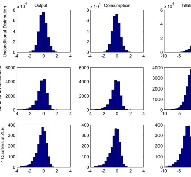
We now document how the endogenous variables behave while the economy is at the ZLB. Fig. 7 compares the distributions of consumption, output, and inflation. The first row represents the unconditional distribution of the three variables. In particular,

μ

ðvariabletÞforvariabletAfc;y;

Π

gto be approximated by

μ

ðfvariabletAAgÞC

PT

i¼1IAðvariableðSi;ssÞÞ

T

20 40 60 80 100

0 2 4 6 8

Interest Rate

20 40 60 80 100

-3 -2 -1 0 1 2

Consumption

20 40 60 80 100

-4 -3 -2 -1 0

Labor

20 40 60 80 100

-10 -5 0

Inflation

Non-Linear Approx Linear Approx

for any setAR. The second row shows the same distribution conditional on being at the ZLB, approximating it by

μ

ðfvariabletAAgjfRt¼1gÞC

PM

k¼1IAðvariableðSik;ssÞÞ

M :

The third row conditions on being at the ZLB for four periods approximating it by

μ

fvariabletAAgjRt1;4

C

PM4

k4¼1IA variable Sik4;ss

M4 :

The three distributions are negatively skewed: the ZLB is associated with low consumption, output, and inflation. When at the ZLB, consumption is on average 0.23 percent below its value in the steady state with positive inflation, output is 0.25 percent below, and inflation is 1.89 percent (in annualized terms), 4 percentage points less than its average at the unconditional distribution (2.1 percent). The distributions are even more skewed if we condition on being at the ZLB for four periods. The average values also get more negative. Consumption is on average 0.34 percent below and output is 0.32 percent below their steady-state values, and inflation is 2.83 percent (in annualized terms). We should not read the previous numbers as suggesting that the ZLB is a mild illness: in some bad events, the ZLB makes output drop 8.6 percent, consumption falls 8.2 percent, and inflation is13.5 percent. Given our rich stochastic structure, a spell at the ZLB is not always associated with deflation. Out of the 300,000 simulations, our economy is at the ZLB in 16,588 periods, and in 562 of those, inflation is positive (around 3 percent), with an annualized average value of 0.29 percent.

0 10 20 30 40 50 60 70 80 90 100 -25

-20 -15 -10 -5 0 5 10

Constrained Interest Rate Unconstrained Interest Rate

Fig. 6.Constrained versus unconstrained interest rate.

Table 5

Endogenous variables and shocks at the ZLB.

ct=c lt=l yt=y Πt

4

βt At sg;t mt

b

EðÞ 0.999 1.001 0.999 1.021 0.994 1.000 0.200 1.000

b

EðjRt1;1Þ 0.999 0.992 0.998 0.986 1.000 1.007 0.200 0.999

b

EðjRt1;4Þ 0.996 0.989 0.996 0.974 1.000 1.009 0.200 0.999

d

StdðÞ 0.0059 0.0048 0.0059 0.0173 0.0041 0.0058 0.0008 0.0025

d

StdðjRt1;1Þ 0.0064 0.0038 0.0064 0.0094 0.0031 0.0044 0.0008 0.0025

d

StdðjRt1;4Þ 0.0082 0.0063 0.0082 0.0158 0.0033 0.0047 0.0008 0.0025

Table 6

Unconditional and conditional moments of exogenous states.

σb Expected periods at ZLB Standard dev. of periods at ZLB Multiplier

0.0027 4 2.04 1.97

0.0025 4 2.08 1.76

Table 5provides further information about the endogenous variables and shocks at the ZLB at different horizons. The rows indicate the conditioning set. Rt1;i means that the economy has been at the ZLB i quarters. So, for instance, conditional on being at the ZLB for 4 quarters, consumption is 0.4 percent below its steady-state value and annualized inflation

Π

t

4

is2.6 percent a year. Similarly, the demand shock and productivity are high. In other words, spells at the ZLB tend to be generated by these two forces. In comparison, monetary policy shocks play a relatively small role in pushing the economy to the ZLB (Table 6).

5.7. The size of the fiscal multiplier

Woodford (2011)andChristiano et al. (2011)have argued that, at the ZLB, fiscal multipliers might be large. We use our model to show the importance of nonlinearities in assessing the size of these multipliers. When the economy is outside the ZLB, we proceed as follows:

1. We find the unconditional means of output,y1, and government spending,g1.

2. Starting at those points, we increase g1 by 1 percent, 10 percent, 20 percent, and 30 percent (that is, if government

consumption is 1, we raise it to either 1.01, 1.1, 1.2, or 1.3). As time goes by,sg;tfollows its law of motion(2)back to its average level.

3. For each increase in government spending, we simulate the economy. Letyg;tandgg;t denote the new simulated paths. 4. We compute the multiplierðyg;ty1=gg;1g1Þ:

Since the model is nonlinear, the multiplier depends on the point at which we make our computation. A natural candidate is the unconditional mean of the states. Also, we calculate the response of the economy to different increases in government consumption because, when we solve the model nonlinearly, the marginal multiplier(the multiplier when government consumption goes up by an infinitesimal amount) is different from theaverage multiplier(the multiplier when government consumption goes up by a discrete number; see alsoErceg and Lindé, 2010). We approximate the marginal multiplier with the multiplier that increases government consumption by 1 percent. The other three higher increases give

-4

-2

0

2

4

0

2

4

6

8

x 10

4

Output

n

oit

u

bir

t

si

D

l

a

n

oit

i

d

n

o

c

n

U

0

-4

-2

0

2

4

2

4

6

8

x 10

4

Consumption

-10

-5

0

5

0

2

4

6

x 10

4

Inflation

-4

-2

0

2

4

0

2000

4000

6000

n

oit

u

bir

t

si

D

l

a

n

oit

i

d

n

o

C

-4

-2

0

2

4

0

2000

4000

6000

-10

-5

0

5

0

1000

2000

3000

4000

-4

-2

0

2

4

0

100

200

300

400

B

L

Z

t

a

sr

etr

a

u

Q

4

n

o

l

a

n

oit

i

d

n

o

C

-4

-2

0

2

4

0

100

200

300

400

-10

-5

0

5

0

100

200

300

400

us an idea of how the average multiplier changes with the size of the increment in government consumption. To compute the multiplier at the ZLB

1. We start at the unconditional mean of states except that, to force the economy into the ZLB, we set the discount factor 2 percent above its unconditional mean (at 1.014 instead of the calibrated mean 0.994). This shock sends the economy to the ZLB, on average, for 4 consecutive quarters in the absence of any additional shocks. We select an average duration of 4 quarters to be close to other papers in the literature. We call these unconditional means, output, y1

zlb

, and government spending,gzlb

1 .

2. With these states, we simulate the economy and store the time paths for output,ytzlb, and government spending,gtzlb. 3. With the same states, except that we consider an increase in government consumption at impact of 1 percent, 10 percent,

20 percent, and 30 percent relative to its unconditional mean, we simulate the economy. As time goes by,szlb

g;t follows its law of motion. Letyzlb

g;t andgzlbg;t denote the new simulated paths. 4. We compute the multiplierðyzlb

g;tyzlbt =gzlbg;1g

zlb

1 Þ.

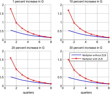
We plot our results inFig. 8: the blue line is the multiplier outside the ZLB and the red crossed line the multiplier at the ZLB. Outside the ZLB, the value of the multiplier at impact is around 0.5 (going from 0.54 when the increment is 1 percent to 0.47 when the increment is 30 percent). We highlight two points. First, the multiplier is small, but not unusual in New Keynesian models with a low labor elasticity, without liquidity-constrained households, and with a Taylor rule that responds to the output gap.5This value is also consistent withWoodford (2011). Second, the difference between the marginal and the average multiplier is small. This is just another manifestation of the near linearity of the model in that situation. At the ZLB, the multiplier of government consumption at impact is much larger: 1.76 for increases in government consumption of 1 percent, 1.68 for increases of 10 percent, 1.59 for increases of 20 percent, and 1.50 for increases of 30 percent. Several patterns are apparent from the red lines inFig. 8. First, the multiplier at the ZLB is significantly above one, albeit smaller than the values reported byChristiano et al. (2011). Second, the multiplier declines as the size of the government shock

0

2

4

6

8

0

0.5

1

1.5

2

1 percent increase in G

0

2

4

6

8

0

0.5

1

1.5

2

10 percent increase in G

0

2

4

6

8

0

0.5

1

1.5

2

20 percent increase in G

quarters

0

2

4

6

8

0

0.5

1

1.5

2

30 percent increase in G

quarters

Multiplier w ithout ZLB Multiplier w ith ZLB

Fig. 8.Government spending multiplier when the ZLB lasts 4 quarters on average. (For interpretation of the references to color in this figure caption, the reader is referred to the web version of this paper.)

5

increases. As the government shock increases, the expected number of periods at the ZLB decreases for a given discount factor shock. In our experiment, a 30 percent government shock pushes the economy, on average, out of the ZLB upon impact. This suggests that we must be careful when we read the empirical evidence on fiscal multipliers, as their estimated value may depend on the size of the observed changes in government consumption, something that a structural vector autoregression (SVAR) will not be able to capture.

Why are our multipliers smaller than the one reported byChristiano et al. (2011)? Because our exercise is different. First, we have a rich stochastic structure in our model: in any period the economy is hit by several shocks. Agents do not have perfect foresight and the distribution of the number of periods at the ZLB is not degenerate. Second, the government expenditure follows its law of motion(2) regardless of whether the economy is at the ZLB. So, for instance, if a large government consumption shock pushes the economy out of the ZLB right away, government consumption would still be high for many quarters, lowering the multiplier (Christiano et al., 2011, also show a similar result). Our experiment complements other exercises in the literature by evaluating the fiscal multiplier in an empirically relevant scenario: when neither governments nor agents know how long the economy will be at the ZLB and government expenditure is persistent. Let us now analyze how the nondegenerate distribution of the number of periods at the ZLB that the agents face affects our results. To do this, we solve three versions of the model with three levels of volatility for the discount factor shock (column 1 ofTable 5). In each of the three cases, we increase—at time zero—the discount factor so that, on average, the economy stays at the ZLB for 4 periods. We report the standard deviation of the periods at the ZLB (third column) and the impact fiscal multiplier (fourth column). To compute these numbers, we simulate the economy 5000 times for each version of our model. As we reduce

σ

b, the multiplier falls and the standard deviation of the number of periods at the ZLB grows.

Because of the left censoring of the spell duration, even if the expected durations of the ZLB spell are constant across the three experiments, a higher standard deviation of the number of periods at the ZLB means a higher probability of ZLB spell durations shorter than four periods. For instance, this probability increases four percentage points from

σ

b¼0:0027 to

σ

b¼0:00175. Since, in these events,gtpushes interest rates up, the total effect of additional government expenditure on aggregate demand today is much lower.

To evaluate how the expected number of periods at the ZLB affects the fiscal multiplier,Fig. 9shows the results when the discount factor is initially set to be 1.2 percent above its unconditional mean. This sends the economy to the ZLB, in the absence of additional shocks, on average for 2 quarters. The multiplier outside the ZLB is the same as before. But the multiplier at the ZLB is now smaller at only around 2 times larger than in normal times. For an increment of 1 percent in government expenditure, the impact multiplier is 1.20, and it goes down to 1.00 when the increment is 30 percent. Thus,

0 2 4 6 8

0 0.5 1 1.5

1 percent increase in G

0 2 4 6 8

0 0.5 1 1.5

10 percent increase in G

0 2 4 6 8

0 0.5 1 1.5

20 percent increase in G

quarters

0 2 4 6 8

0 0.5 1 1.5

30 percent increase in G

quarters

Multiplier without ZLB Multiplier with ZLB

Fig. 9illustrates how the size of the fiscal multiplier depends on the expected duration of the spell at the ZLB without fiscal shocks (Christiano et al., 2011, document this point as well). The intuition, which we will develop in the next section, comes from the Euler equation forwarded several periods. The longer we are expected to stay at the ZLB, the lower is the current demand for consumption (lower consumption in the future imposes, by optimality, lower consumption today). For completeness, in the appendix, we include additional IRFs of the model to a government expenditure shock.

6. Extending the length of spells at the ZLB

Table 2shows that the spells at the ZLB in our simulation tend to be shorter than the recent experiences of the U.S., Europe, and Japan. Now we analyze why this is the case and how we can fix the model to change this result.

Recall that, at the ZLB, the household's Euler equation is

1

ct

¼Et

β

tþ1

ctþ1

Π

tþ1:

This equation can we rewritten as

1

ct

¼Et

δ

t 1

ctþ1

ð13Þ

where

δ

t¼

Et

β

tþ1

ctþ1

Π

tþ1

Et 1

ctþ1

:

AsSection 5showed, the ZLB is associated with deflation and a high

β

t. Hence, at the ZLB, we will generally have that

δ

t41. Iterating on Eq.(13)forNquarters

1

ct

¼Et

δ

t

δ

tþ1…

δ

tþN1 1

ctþN:

ð14Þ

6.1. Length of spells at the ZLB vs. drops in consumption

Equation(14)uncovers a basic tension in our model. We either match the recent large spell at the ZLB and generate a huge drop in consumption, or we match the observed moderate drop in consumption and accept a short expected spell at the ZLB.

A first way to see this is to note that ifctþNc(i.e., the household expects that the economy will be close to the steady state when it leaves the ZLB attþN), we have

ct 1

Et∏t_τþ¼Nt1

δ

τ

c:

IfNis large (i.e., the economy is at the ZLB for a long time), even expected values of

δ

tonly slightly above 1 bring a large drop

in consumption because they get amplified by the factor∏tþN1

τ¼t

δ

τ. For instance, in our calibration, the conditional mean of

δ

tat the ZLB is 1.0019. If the household expects this value of

δ

tfor 40 quarters and, then, a reversion toc, consumption today

would drop by approximately 7.4 percentð ¼1=1:001940Þwith respect to the steady state. However, in the data, the drop in consumption has been more modest. Consumption per capita only fell 4.2 percent in the U.S. between its peak on 2007.Q3 and its trough in 2009.Q2, and it has been growing uninterruptedly from 2009.Q4 until 2015.Q1, despite the ZLB still being binding. In our long simulation, we sometimes get large values of

δ

t, but their expectation quickly reverts below 1: the

simulated expected duration of the spell at the ZLB is only 2.06 quarters. Thus, the associated drops in consumption are usually small as well. Even in the“lost decade”mentioned inSection 5.5, the largest drop in consumption is just 3.3 percent relative to the steady state.

A comparison with Aiyagari (1994)is instructive. In that model, the term analogous to

δ

t in the household's Euler

equation would be

β

RwhereRis the real return to capital net of depreciation. Any steady state in such a model must have

β

Ro1 to ensure that aggregate savings do not grow without bound. In our model, there is a similar feature. If

δ

t41, the household's desire to save generally results inctoctþ1. If

δ

tis persistently greater than one, going backwards in time results

in consumption gravitating toward zero.

A second way to illustrate the challenge of generating long spells at the ZLB without a massive drop in consumption is by considering a simplified version of the model where the only shock is

β

tand Calvo pricing has been replaced by Rotemberg

element for every value of

β

t. We use price stickiness parameter values such that the linearized Calvo and Rotemberg models

are observationally equivalent. Beginning with the initial guess that the consumption, inflation, and interest rate decision rules are equal to the steady-state values of these variables for all

β

t(flat lines at the top panels and the bottom left panel of

Fig. 10), we iterate backwards as we did in our benchmark solution.

Fig. 10 displays the values ofct,

Π

t, and

δ

t at different iterations for a demand shock persistence of

ρ

b¼0:94 (the unconditional variance is the same as in the benchmark) and a Taylor coefficient for inflation

ϕ

_π¼2:5.Fig. 10shows how, once the iterations are such that the economy is at the ZLB, subsequent iterations quickly drivectdown to zero with a

corresponding decrease in

Π

tand increases in

δ

t. Because of consumption smoothing, a drop inctat states where the ZLB

binds leads to decreased consumption inct1, which increases the likelihood the ZLB will bind in the subsequent iteration.6 This_“death spiral_”is so severe that after a few iterations, consumption goes to zero. Why do we avoid this catastrophic collapse of the economy in our benchmark calibration? Because we have a lower

ρ

b(0.8), which makes

β

t's travels above one

less persistent, and because we include other shocks, which can get the economy out of the ZLB, even when

β

tis high.

In summary, within the framework of the standard New Keynesian model, one can either generate long spells at the ZLB with catastrophic drops in consumption or one can generate short spells at the ZLB with moderate drops in consumption. But one cannot get long spells at the ZLB with moderate drops in consumption.

6.2. Generating long spells at the ZLB

How can we get around the results in the previous subsection? The natural solution is to break the Euler equation. A transparent mechanism to do so is to introduce a wedge in Eq.(13). Since, in the interest of space, we do not want to formulate a whole new model, we consider a simple device that nevertheless illuminates the mechanism at work: a tax on savings.7_{Specifically, assuming the household faces a tax}

τ

tproportional to the gross nominal return on bonds, the Euler

0.99 0.995 1 1.005

0.2 0.3 0.4 0.5 0.6 0.7 0.8

0.9

Consumption

0.99 0.995 1 1.005

0.88 0.9 0.92 0.94 0.96 0.98 1

1.02

Inflation

t t

0.99 0.995 1 1.005

1 1.005 1.01 1.015 1.02

1.025

Interest Rate

0.99 0.995 1 1.005

0.96 0.98 1 1.02 1.04 1.06 1.08 1.1 1.12

Fig. 10.Collapsing economy at the ZLB.

6

Note that when government consumption is a small percentage of output and since, in this simplified model, we forget about the monetary policy shock, we haveZtct=c ϕyΠt=Π ϕπ. Thus, a smallctlowersZtand increases the probability that the ZLB binds.

7

equation becomes

1

ct¼Rtð1

τ

tÞEt

β

tþ1

ctþ1

Π

tþ1:

Just for convenience in our exposition, let us also assume that

τ

t¼

0 ifEtctþβ1tΠþ1tþ14

1

γc

11

γc Etctþβ1tΠþ1tþ1

1

otherwise :

8 > <

> :

Then, we can write the Euler equation as

1

ct

¼Rtmin Et

β

tþ1

ctþ1

Π

tþ1; 1

γ

c

:

By choosing

γ

, one can control the strength of the_“death spiral_”: at the ZLB, 1₌ctr1=ð

γ

cÞ; implyingctZ

γ

c. This also essentially forces

Π

_τtþ¼Nt1

δ

τr

γ

1for any spell length.8

We set

γ

¼0:99 and repeat, inFig. 11, the same exercise as inFig. 10Once the tax on savings is in place, consumption no longer gravitates toward zero. While on the first iterations consumption falls drastically, the tax on savings eventually prevents consumption from collapsing: the dark starred lines correspond to the policy functions once convergence has been achieved. It also limits the spread of reduced consumption to other states. In fact, one can increase the persistence of the shock virtually without bound and still obtain convergence.

We document this last remark withTable 7and two experiments using our benchmark model with an Euler equation wedge. First, we increase the persistence of the demand shock while also sometimes increasing

ϕ

_π to prevent explosive inflation.9For

γ

¼0:95, increasing

ρ

bto 0.95 and

ϕ

_πto 2.5 raises the expected duration of a ZLB spell to 8.7 quarters. If one

0.99 0.995 1 1.005

0.806 0.808 0.81 0.812 0.814 0.816

0.818 Consumption

0.99 0.995 1 1.005

0.985 0.99 0.995 1 1.005

1.01 Inflation

t

0.99 0.995 1 1.005

1 1.005 1.01 1.015 1.02

Interest Rate

t

0.99 0.995 1 1.005

0.98 0.985 0.99 0.995 1 1.005 1.01 1.015 1.02

Fig. 11.Policy iterations with savings tax.

8_{A perhaps more natural case would be to design a tax on savings that enforcesδ}

t¼1 at the ZLB. However, this rule induces indeterminacy, since one then obtains 1=ct¼Etð1=ctþ1Þ;and marginal utility becomes a random walk.

9

pushes

ρ

bto 0.998, the expected duration increases to 36.4 quarters, roughly a decade. Second, we lower the inflation target

below one. The result is dramatic: even for

ρ

b¼0:8, the economy isalways at the ZLB, the constraint 1=ctr1=ð

γ

cÞ is constantly binding, and we have an annualized 24 percent deflation. In a less drastic case where

ρ

b¼0:95 (and therefore a long sequence of low

β

tvalues occurs with non-negligible probability), the ZLB occurs 99 percent of the time and the

expected duration of a spell is 195 quarters. In all these cases, as in our benchmark calibration, the expected number of additional periods at the ZLB is increasing in the time spent there. This is seen in the statistic

b

EðTt1jRt1;8Þ=bEðTt1jRt1;1Þ, whose value ranges from 1.65 to 2.80.

The results inTable 7 also have an interesting empirical implication. While in our benchmark calibration, we get a realistic inflation mean of 2.4 percent when the economy is away from the ZLB (compared to the data's 2.5 percent), we miss inflation at the ZLB. The mean annualized inflation rate at the ZLB in our benchmark calibration is 1.9 percent; the annualized inflation rate in the U.S. from 2008.Q4 (when the U.S. entered the ZLB) to 2015.Q1 has been 1.4 percent.10_{If the} model predicted positive inflation rather than deflation at the ZLB,

δ

twould be smaller, effectively acting as a positive

savings tax at the ZLB like the one used to generate Table 7. One avenue for future research is, therefore, to find a modification of the model that can simultaneously capture inflation dynamics at and away from the ZLB.

There are, of course, alternative ways to break away from the Euler equation (14). A first possibility is to have heterogeneous households (either through overlapping generations or through incomplete markets). A second possibility is to have labor market frictions that prevent labor and output from rapidly adjusting. A third possibility is to explore the role of government spending propping up aggregate demand in recessions. Finally, international transmission mechanisms might act as an additional boost to aggregate demand. More research is needed to determine which, if any, of these stories is capable of bringing the model closer to the data.

7. Conclusion

Our paper demonstrates the importance of nonlinearities when the economy is at the ZLB. Several lines of future research lay ahead. First, we could repeat our analysis with larger models that are closer to the ones used by central banks for practical policymaking. Second, we could extend our model to include a richer set of fiscal policy instruments. Since the ZLB is a situation in which households are already saving too much, reductions in taxes financed through debt may have little bite. Third, we could mix our solution with a particle filter to build the likelihood function for estimation as in

Fernández-Villaverde and Rubio-Ramírez (2007). Estimating this class of models with a full-likelihood approach is promising (Gust et al., 2012). We can use the information in the data about parameters describing preferences and technology to evaluate the behavior of the model at the ZLB, something that SVARs would have a harder time doing because the U.S. has been at the ZLB only once since World War II. If the U.S. stays at or close to the ZLB in the near future, these next steps are a high priority.

Table 7

ZLB statistics with limited liquidity traps.

Parameters Statistics

γ ρb Π ϕπ cPrðfRt¼1gÞ bEðTtjRt1;1Þ dStdðTtjRt1;1Þ bEðTt1jRt1;8Þ b

EðTt1jRt1;1Þ

– – – – 5.53 2.06 1.82 1.81

0.95 – – – 5.53 2.06 1.82 1.81

0.95 0.95 0.995 – 98.6 194.7 322.3 1.65

0.95 0.9