Ian Robinson,
2n
d E
ditio
n
NEW OPPORTUNITIES FOR CONNECTED DATA
Graph
Databases
Com
978-1-491-93200-1 [LSI]
Graph Databases
by Ian Robinson, Jim Webber, and Emil Eifrem
Copyright © 2015 Neo Technology, Inc. All rights reserved. Printed in the United States of America.
Published by O’Reilly Media, Inc., 1005 Gravenstein Highway North, Sebastopol, CA 95472.
O’Reilly books may be purchased for educational, business, or sales promotional use. Online editions are also available for most titles (http://safaribooksonline.com). For more information, contact our corporate/ institutional sales department: 800-998-9938 or [email protected].
Editor: Marie Beaugureau
Production Editor: Kristen Brown
Proofreader: Christina Edwards
Indexer: WordCo Indexing Services
Interior Designer: David Futato
Cover Designer: Ellie Volckhausen
Illustrator: Rebecca Demarest
June 2013: First Edition June 2015: Second Edition
Revision History for the Second Edition
2015-05-04: First Release
See http://oreilly.com/catalog/errata.csp?isbn=9781491930892 for release details.
The O’Reilly logo is a registered trademark of O’Reilly Media, Inc. Graph Databases, the cover image of an European octopus, and related trade dress are trademarks of O’Reilly Media, Inc.
Table of Contents
Foreword. . . vii
Preface. . . xi
1. Introduction. . . 1
What Is a Graph? 1
A High-Level View of the Graph Space 4
Graph Databases 5
Graph Compute Engines 7
The Power of Graph Databases 8
Performance 8
Flexibility 9
Agility 9
Summary 10
2. Options for Storing Connected Data. . . 11
Relational Databases Lack Relationships 11
NOSQL Databases Also Lack Relationships 15
Graph Databases Embrace Relationships 18
Summary 24
3. Data Modeling with Graphs. . . 25
Models and Goals 25
The Labeled Property Graph Model 26
Querying Graphs: An Introduction to Cypher 27
Cypher Philosophy 28
MATCH 30
Other Cypher Clauses 31
A Comparison of Relational and Graph Modeling 32
Relational Modeling in a Systems Management Domain 33
Graph Modeling in a Systems Management Domain 38
Testing the Model 39
Cross-Domain Models 41
Creating the Shakespeare Graph 45
Beginning a Query 46
Declaring Information Patterns to Find 48
Constraining Matches 49
Processing Results 50
Query Chaining 51
Common Modeling Pitfalls 52
Email Provenance Problem Domain 52
A Sensible First Iteration? 52
Second Time’s the Charm 55
Evolving the Domain 58
Identifying Nodes and Relationships 63
Avoiding Anti-Patterns 63
Summary 64
4. Building a Graph Database Application. . . 65
Data Modeling 65
Describe the Model in Terms of the Application’s Needs 66
Nodes for Things, Relationships for Structure 67
Fine-Grained versus Generic Relationships 67
Model Facts as Nodes 68
Represent Complex Value Types as Nodes 71
Time 72
Iterative and Incremental Development 74
Application Architecture 76
Embedded versus Server 76
Clustering 81
Load Balancing 82
Testing 85
Test-Driven Data Model Development 85
Performance Testing 91
Capacity Planning 95
Optimization Criteria 95
Performance 96
Redundancy 98
Importing and Bulk Loading Data 99
Initial Import 99
Batch Import 100
Summary 104
5. Graphs in the Real World. . . 105
Why Organizations Choose Graph Databases 105
Common Use Cases 106
Social 106
Recommendations 107
Geo 108
Master Data Management 109
Network and Data Center Management 109
Authorization and Access Control (Communications) 110
Real-World Examples 111
Social Recommendations (Professional Social Network) 111
Authorization and Access Control 123
Geospatial and Logistics 132
Summary 147
6. Graph Database Internals. . . 149
Native Graph Processing 149
Native Graph Storage 152
Programmatic APIs 158
Kernel API 158
Core API 159
Traversal Framework 160
Nonfunctional Characteristics 162
Transactions 162
Recoverability 163
Availability 164
Scale 166
Summary 170
7. Predictive Analysis with Graph Theory. . . 171
Depth- and Breadth-First Search 171
Path-Finding with Dijkstra’s Algorithm 173
The A* Algorithm 181
Graph Theory and Predictive Modeling 182
Triadic Closures 182
Structural Balance 184
Summary 190
A. NOSQL Overview. . . 193
Foreword
Graphs Are Everywhere, or the Birth of Graph Databases
as We Know Them
It was 1999 and everyone worked 23-hour days. At least it felt that way. It seemed like each day brought another story about a crazy idea that just got millions of dollars in funding. All our competitors had hundreds of engineers, and we were a 20-ish person development team. As if that was not enough, 10 of our engineers spent the majority of their time just fighting the relational database.
It took us a while to figure out why. As we drilled deeper into the persistence layer of our enterprise content management application, we realized that our software was managing not just a lot of individual, isolated, and discrete data items, but also the
connections between them. And while we could easily fit the discrete data in relational tables, the connected data was more challenging to store and tremendously slow to query.
Out of pure desperation, my two Neo cofounders, Johan and Peter, and I started experimenting with other models for working with data, particularly those that were centered around graphs. We were blown away by the idea that it might be possible to replace the tabular SQL semantic with a graph-centric model that would be much easier for developers to work with when navigating connected data. We sensed that, armed with a graph data model, our development team might not waste half its time fighting the database.
1For the younger readers, it may come as a shock that there was a time in the history of mankind when Google didn’t exist. Back then, dinosaurs ruled the earth and search engines with names like AltaVista, Lycos, and Excite were used, primarily to find ecommerce portals for pet food on the Internet.
Well, we AltaVistad1 around the young Web and couldn’t find any. After a few months of surveying, we (naively) set out to build, from scratch, a database that worked natively with graphs. Our vision was to keep all the proven features from the relational database (transactions, ACID, triggers, etc.) but use a data model for the 21st century. Project Neo was born, and with it graph databases as we know them today.
The first decade of the new millennium has seen several world-changing new busi‐ nesses spring to life, including Google, Facebook, and Twitter. And there is a com‐ mon thread among them: they put connected data—graphs—at the center of their business. It’s 15 years later and graphs are everywhere.
Facebook, for example, was founded on the idea that while there’s value in discrete information about people—their names, what they do, etc.—there’s even more value in the relationships between them. Facebook founder Mark Zuckerberg built an empire on the insight to capture these relationships in the social graph.
Similarly, Google’s Larry Page and Sergey Brin figured out how to store and process not just discrete web documents, but how those web documents are connected. Goo‐ gle captured the web graph, and it made them arguably the most impactful company of the previous decade.
Today, graphs have been successfully adopted outside the web giants. One of the big‐ gest logistics companies in the world uses a graph database in real time to route phys‐ ical parcels; a major airline is leveraging graphs for its media content metadata; and a top-tier financial services firm has rewritten its entire entitlements infrastructure on Neo4j. Virtually unknown a few years ago, graph databases are now used in industries as diverse as healthcare, retail, oil and gas, media, gaming, and beyond, with every indication of accelerating their already explosive pace.
I hope this book will serve as a great introduction to this wonderful emerging world of graph technologies, and I hope it will inspire you to start using a graph database in your next project so that you too can unlock the extraordinary power of graphs. Good luck!
Preface
Graph databases address one of the great macroscopic business trends of today: lever‐ aging complex and dynamic relationships in highly connected data to generate insight and competitive advantage. Whether we want to understand relationships between customers, elements in a telephone or data center network, entertainment producers and consumers, or genes and proteins, the ability to understand and ana‐ lyze vast graphs of highly connected data will be key in determining which companies outperform their competitors over the coming decade.
For data of any significant size or value, graph databases are the best way to represent and query connected data. Connected data is data whose interpretation and value requires us first to understand the ways in which its constituent elements are related. More often than not, to generate this understanding, we need to name and qualify the connections between things.
Although large corporations realized this some time ago and began creating their own proprietary graph processing technologies, we’re now in an era where that tech‐ nology has rapidly become democratized. Today, general-purpose graph databases are a reality, enabling mainstream users to experience the benefits of connected data without having to invest in building their own graph infrastructure.
technologies; and by the introduction of general-purpose graph databases into the technology landscape.
About the Second Edition
The first edition of this book was written while Neo4j 2.0 was under active develop‐ ment, when the final forms of labels, indexes, and constraints were still to be fixed. Now that Neo4j is well into its 2.x lifecycle (2.2 at the time of writing, with 2.3 coming soon), we can confidently incorporate the new elements of the graph property model into the text.
For the second edition of this book, we’ve revised all the Cypher examples to bring them in line with the latest Cypher syntax. We’ve added labels both to the queries and the diagrams, and have provided explanations of Cypher’s declarative indexing and optional constraints. Elsewhere, we’ve added additional modeling guidelines, brought the description of Neo4j’s internals up to date with the changes to its internal archi‐ tecture, and updated the testing examples to use the latest tooling.
About This Book
The purpose of this book is to introduce graphs and graph databases to technology practitioners, including developers, database professionals, and technology decision makers. Reading this book will give you a practical understanding of graph databases. We show how the graph model “shapes” data, and how we query, reason about, understand, and act upon data using a graph database. We discuss the kinds of prob‐ lems that are well aligned with graph databases, with examples drawn from actual real-world use cases, and we show how to plan and implement a graph database solu‐ tion.
Conventions Used in This Book
The following typographical conventions are used in this book:
Italic
Indicates new terms, URLs, email addresses, filenames, and file extensions. Constant width
Used for program listings, as well as within paragraphs to refer to program ele‐ ments such as variable or function names, databases, data types, environment variables, statements, and keywords.
Constant width bold
Constant width italic
Shows text that should be replaced with user-supplied values or by values deter‐ mined by context.
This icon signifies a tip, suggestion, or general note.
This icon indicates a warning or caution.
Using Code Examples
Supplemental material (code examples, exercises, etc.) is available for download at https://github.com/iansrobinson/graph-databases-use-cases.
This book is here to help you get your job done. In general, if example code is offered with this book, you may use it in your programs and documentation. You do not need to contact us for permission unless you’re reproducing a significant portion of the code. For example, writing a program that uses several chunks of code from this book does not require permission. Selling or distributing a CD-ROM of examples from O’Reilly books does require permission. Answering a question by citing this book and quoting example code does not require permission. Incorporating a signifi‐ cant amount of example code from this book into your product’s documentation does require permission.
We appreciate, but do not require, attribution. An attribution usually includes the title, author, publisher, and ISBN. For example: “Graph Databases by Ian Robinson, Jim Webber, and Emil Eifrem (O’Reilly). Copyright 2015 Neo Technology, Inc., 978-1-491-93089-2.”
If you feel your use of code examples falls outside fair use or the permission given above, feel free to contact us at [email protected].
Safari® Books Online
Technology professionals, software developers, web designers, and business and crea‐ tive professionals use Safari Books Online as their primary resource for research, problem solving, learning, and certification training.
Safari Books Online offers a range of plans and pricing for enterprise, government, education, and individuals.
Members have access to thousands of books, training videos, and prepublication manuscripts in one fully searchable database from publishers like O’Reilly Media, Prentice Hall Professional, Addison-Wesley Professional, Microsoft Press, Sams, Que, Peachpit Press, Focal Press, Cisco Press, John Wiley & Sons, Syngress, Morgan Kauf‐ mann, IBM Redbooks, Packt, Adobe Press, FT Press, Apress, Manning, New Riders, McGraw-Hill, Jones & Bartlett, Course Technology, and hundreds more. For more information about Safari Books Online, please visit us online.
How to Contact Us
Please address comments and questions concerning this book to the publisher: O’Reilly Media, Inc.
1005 Gravenstein Highway North Sebastopol, CA 95472
800-998-9938 (in the United States or Canada) 707-829-0515 (international or local)
707-829-0104 (fax)
We have a web page for this book, where we list errata, examples, and any additional information. You can access this page at http://bit.ly/graph-databases-2e.
To comment or ask technical questions about this book, send email to bookques‐ [email protected].
For more information about our books, courses, conferences, and news, see our web‐ site at http://www.oreilly.com.
Find us on Facebook: http://facebook.com/oreilly Follow us on Twitter: http://twitter.com/oreillymedia Watch us on YouTube: http://www.youtube.com/oreillymedia
Acknowledgments
We would like to thank our technical reviewers: Michael Hunger, Colin Jack, Mark Needham, and Pramod Sadalage.
Our colleagues at Neo Technology have contributed enormously of their time, experi‐ ence, and effort throughout the writing of this book. Thanks in particular go to Anders Nawroth, for his invaluable assistance with our book’s toolchain; Andrés Tay‐ lor, for his enthusiastic help with all things Cypher; and Philip Rathle, for his advice and contributions to the text.
A big thank you to everyone in the Neo4j community for your many contributions to the graph database space over the years.
And special thanks to our families, for their love and support: Lottie, Tiger, Elliot, Kath, Billy, Madelene, and Noomi.
1For introductions to graph theory, see Richard J. Trudeau, Introduction To Graph Theory (Dover, 1993) and Gary Chartrand, Introductory Graph Theory (Dover, 1985). For an excellent introduction to how graphs pro‐ vide insight into complex events and behaviors, see David Easley and Jon Kleinberg, Networks, Crowds, and Markets: Reasoning about a Highly Connected World (Cambridge University Press, 2010).
CHAPTER 1
Introduction
Although much of this book talks about graph data models, it is not a book about graph theory.1 We don’t need much theory to take advantage of graph databases: pro‐ vided we understand what a graph is, we’re practically there. With that in mind, let’s refresh our memories about graphs in general.
What Is a Graph?
Graphs Are Everywhere
Graphs are extremely useful in understanding a wide diversity of datasets in fields such as science, government, and business. The real world—unlike the forms-based model behind the relational database—is rich and interrelated: uniform and rule-bound in parts, exceptional and irregular in others. Once we understand graphs, we begin to see them in all sorts of places. Gartner, for example, identifies five graphs in the world of business—social, intent, consumption, interest, and mobile—and says that the ability to leverage these graphs provides a “sustainable competitive advan‐ tage.”
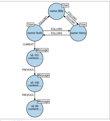
For example, Twitter’s data is easily represented as a graph. In Figure 1-1 we see a small network of Twitter users. Each node is labeled User, indicating its role in the network. These nodes are then connected with relationships, which help further establish the semantic context: namely, that Billy follows Harry, and that Harry, in turn, follows Billy. Ruth and Harry likewise follow each other, but sadly, although Ruth follows Billy, Billy hasn’t (yet) reciprocated.
Figure 1-1. A small social graph
Figure 1-2. Publishing messages
The Labeled Property Graph Model
In discussing Figure 1-2 we’ve also informally introduced the most popular form of graph model, the labeled property graph (in Appendix A, we discuss alternative graph data models in more detail). A labeled property graph has the following characteris‐ tics:
• It contains nodes and relationships. • Nodes contain properties (key-value pairs). • Nodes can be labeled with one or more labels.
• Relationships are named and directed, and always have a start and end node. • Relationships can also contain properties.
Most people find the property graph model intuitive and easy to understand. Although simple, it can be used to describe the overwhelming majority of graph use cases in ways that yield useful insights into our data.
A High-Level View of the Graph Space
Numerous projects and products for managing, processing, and analyzing graphs have exploded onto the scene in recent years. The sheer number of technologies makes it difficult to keep track of these tools and how they differ, even for those of us who are active in the space. This section provides a high-level framework for making sense of the emerging graph landscape.
From 10,000 feet, we can divide the graph space into two parts:
Technologies used primarily for transactional online graph persistence, typically accessed directly in real time from an application
These technologies are called graph databases and are the main focus of this book. They are the equivalent of “normal” online transactional processing (OLTP) databases in the relational world.
Technologies used primarily for offline graph analytics, typically performed as a series of batch steps
2See Rodriguez, Marko A., and Peter Neubauer. 2011. “The Graph Traversal Pattern.” In Graph Data Manage‐ ment: Techniques and Applications, ed. Sherif Sakr and Eric Pardede, 29-46. Hershey, PA: IGI Global.
Another way to slice the graph space is to look at the graph models employed by the various technologies. There are three dominant graph data models: the property graph, Resource Description Framework (RDF) triples, and hypergraphs. We describe these in detail in Appendix A. Most of the popular graph databases on the market use a variant of the property graph model, and conse‐ quently, it’s the model we’ll use throughout the remainder of this book.
Graph Databases
A graph database management system (henceforth, a graph database) is an online database management system with Create, Read, Update, and Delete (CRUD) meth‐ ods that expose a graph data model. Graph databases are generally built for use with transactional (OLTP) systems. Accordingly, they are normally optimized for transac‐ tional performance, and engineered with transactional integrity and operational availability in mind.
There are two properties of graph databases we should consider when investigating graph database technologies:
The underlying storage
Some graph databases use native graph storage that is optimized and designed for storing and managing graphs. Not all graph database technologies use native graph storage, however. Some serialize the graph data into a relational database, an object-oriented database, or some other general-purpose data store.
The processing engine
Some definitions require that a graph database use index-free adjacency, meaning that connected nodes physically “point” to each other in the database.2 Here we take a slightly broader view: any database that from the user’s perspective behaves
like a graph database (i.e., exposes a graph data model through CRUD opera‐ tions) qualifies as a graph database. We do acknowledge, however, the significant performance advantages of index-free adjacency, and therefore use the term
It’s important to note that native graph storage and native graph processing are neither good nor bad—they’re simply classic engi‐ neering trade-offs. The benefit of native graph storage is that its purpose-built stack is engineered for performance and scalability. The benefit of nonnative graph storage, in contrast, is that it typi‐ cally depends on a mature nongraph backend (such as MySQL) whose production characteristics are well understood by opera‐ tions teams. Native graph processing (index-free adjacency) bene‐ fits traversal performance, but at the expense of making some queries that don’t use traversals difficult or memory intensive.
[image:24.504.74.431.322.568.2]Relationships are first-class citizens of the graph data model. This is not the case in other database management systems, where we have to infer connections between entities using things like foreign keys or out-of-band processing such as map-reduce. By assembling the simple abstractions of nodes and relationships into connected structures, graph databases enable us to build arbitrarily sophisticated models that map closely to our problem domain. The resulting models are simpler and at the same time more expressive than those produced using traditional relational databases and the other NOSQL (Not Only SQL) stores.
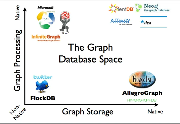
Figure 1-3 shows a pictorial overview of some of the graph databases on the market today, based on their storage and processing models.
Graph Compute Engines
A graph compute engine is a technology that enables global graph computational algo‐ rithms to be run against large datasets. Graph compute engines are designed to do things like identify clusters in your data, or answer questions such as, “how many relationships, on average, does everyone in a social network have?”
Because of their emphasis on global queries, graph compute engines are normally optimized for scanning and processing large amounts of information in batches, and in that respect they are similar to other batch analysis technologies, such as data min‐ ing and OLAP, in use in the relational world. Whereas some graph compute engines include a graph storage layer, others (and arguably most) concern themselves strictly with processing data that is fed in from an external source, and then returning the results for storage elsewhere.
Figure 1-4 shows a common architecture for deploying a graph compute engine. The architecture includes a system of record (SOR) database with OLTP properties (such as MySQL, Oracle, or Neo4j), which services requests and responds to queries from the application (and ultimately the users) at runtime. Periodically, an Extract, Trans‐ form, and Load (ETL) job moves data from the system of record database into the graph compute engine for offline querying and analysis.
Figure 1-4. A high-level view of a typical graph compute engine deployment
This Book Focuses on Graph Databases
The previous section provided a coarse-grained overview of the entire graph space. The rest of this book focuses on graph databases. Our goal throughout is to describe graph database concepts. Where appropriate, we illustrate these concepts with exam‐ ples drawn from our experience of developing solutions using the labeled property graph model and the Neo4j database. Irrespective of the graph model or database used for the examples, however, the important concepts carry over to other graph databases.
The Power of Graph Databases
Notwithstanding the fact that just about anything can be modeled as a graph, we live in a pragmatic world of budgets, project time lines, corporate standards, and commo‐ ditized skillsets. That a graph database provides a powerful but novel data modeling technique does not in itself provide sufficient justification for replacing a well-established, well-understood data platform; there must also be an immediate and very significant practical benefit. In the case of graph databases, this motivation exists in the form of a set of use cases and data patterns whose performance improves by one or more orders of magnitude when implemented in a graph, and whose latency is much lower compared to batch processing of aggregates. On top of this performance benefit, graph databases offer an extremely flexible data model, and a mode of deliv‐ ery aligned with today’s agile software delivery practices.
Performance
Flexibility
As developers and data architects, we want to connect data as the domain dictates, thereby allowing structure and schema to emerge in tandem with our growing understanding of the problem space, rather than being imposed upfront, when we know least about the real shape and intricacies of the data. Graph databases address this want directly. As we show in Chapter 3, the graph data model expresses and accommodates business needs in a way that enables IT to move at the speed of busi‐ ness.
Graphs are naturally additive, meaning we can add new kinds of relationships, new nodes, new labels, and new subgraphs to an existing structure without disturbing existing queries and application functionality. These things have generally positive implications for developer productivity and project risk. Because of the graph model’s flexibility, we don’t have to model our domain in exhaustive detail ahead of time—a practice that is all but foolhardy in the face of changing business requirements. The additive nature of graphs also means we tend to perform fewer migrations, thereby reducing maintenance overhead and risk.
Agility
We want to be able to evolve our data model in step with the rest of our application, using a technology aligned with today’s incremental and iterative software delivery practices. Modern graph databases equip us to perform frictionless development and graceful systems maintenance. In particular, the schema-free nature of the graph data model, coupled with the testable nature of a graph database’s application program‐ ming interface (API) and query language, empower us to evolve an application in a controlled manner.
Summary
In this chapter we’ve reviewed the graph property model, a simple yet expressive tool for representing connected data. Property graphs capture complex domains in an expressive and flexible fashion, while graph databases make it easy to develop appli‐ cations that manipulate our graph models.
CHAPTER 2
Options for Storing Connected Data
We live in a connected world. To thrive and progress, we need to understand and influence the web of connections that surrounds us.
How do today’s technologies deal with the challenge of connected data? In this chap‐ ter we look at how relational databases and aggregate NOSQL stores manage graphs and connected data, and compare their performance to that of a graph database. For readers interested in exploring the topic of NOSQL, Appendix A describes the four major types of NOSQL databases.
Relational Databases Lack Relationships
For several decades, developers have tried to accommodate connected, semi-structured datasets inside relational databases. But whereas relational databases were initially designed to codify paper forms and tabular structures—something they do exceedingly well—they struggle when attempting to model the ad hoc, exceptional relationships that crop up in the real world. Ironically, relational databases deal poorly with relationships.
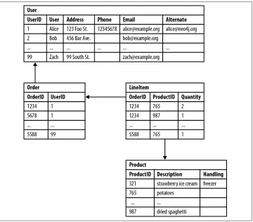
Figure 2-1 shows a relational schema for storing customer orders in a customer-centric, transactional application.
Figure 2-1. Semantic relationships are hidden in a relational database
The application exerts a tremendous influence over the design of this schema, mak‐ ing some queries very easy, and others more difficult:
• Join tables add accidental complexity; they mix business data with foreign key metadata.
• Foreign key constraints add additional development and maintenance overhead
just to make the database work.
• Sparse tables with nullable columns require special checking in code, despite the presence of a schema.
• Several expensive joins are needed just to discover what a customer bought. • Reciprocal queries are even more costly. “What products did a customer buy?” is
the basis of recommendation systems. We could introduce an index, but even with an index, recursive questions such as “which customers buying this product also bought that product?” quickly become prohibitively expensive as the degree of recursion increases.
Relational databases struggle with highly connected domains. To understand the cost of performing connected queries in a relational database, we’ll look at some simple and not-so-simple queries in a social network domain.
Figure 2-2 shows a simple join-table arrangement for recording friendships.
Figure 2-2. Modeling friends and friends-of-friends in a relational database
Asking “who are Bob’s friends?” is easy, as shown in Example 2-1.
Example 2-1. Bob’s friends
SELECT p1.Person
FROM Person p1 JOIN PersonFriend ON PersonFriend.FriendID = p1.ID JOIN Person p2
ON PersonFriend.PersonID = p2.ID WHERE p2.Person = 'Bob'
Based on our sample data, the answer is Alice and Zach. This isn’t a particularly expensive or difficult query, because it constrains the number of rows under consid‐ eration using the filter WHERE Person.person='Bob'.
Friendship isn’t always a reflexive relationship, so in Example 2-2, we ask the recipro‐ cal query, which is, “who is friends with Bob?”
Example 2-2. Who is friends with Bob?
SELECT p1.Person
ON PersonFriend.FriendID = p2.ID WHERE p2.Person = 'Bob'
The answer to this query is Alice; sadly, Zach doesn’t consider Bob to be a friend. This reciprocal query is still easy to implement, but on the database side it’s more expen‐ sive, because the database now has to consider all the rows in the PersonFriend table. We can add an index, but this still involves an expensive layer of indirection. Things become even more problematic when we ask, “who are the friends of my friends?” Hierarchies in SQL use recursive joins, which make the query syntactically and com‐ putationally more complex, as shown in Example 2-3. (Some relational databases pro‐ vide syntactic sugar for this—for instance, Oracle has a CONNECT BY function—which simplifies the query, but not the underlying computational complexity.)
Example 2-3. Alice’s friends-of-friends
SELECT p1.Person AS PERSON, p2.Person AS FRIEND_OF_FRIEND FROM PersonFriend pf1 JOIN Person p1
ON pf1.PersonID = p1.ID JOIN PersonFriend pf2
ON pf2.PersonID = pf1.FriendID JOIN Person p2
ON pf2.FriendID = p2.ID
WHERE p1.Person = 'Alice' AND pf2.FriendID <> p1.ID
This query is computationally complex, even though it only deals with the friends of Alice’s friends, and goes no deeper into Alice’s social network. Things get more com‐ plex and more expensive the deeper we go into the network. Though it’s possible to get an answer to the question “who are my friends-of-friends-of-friends?” in a rea‐ sonable period of time, queries that extend to four, five, or six degrees of friendship deteriorate significantly due to the computational and space complexity of recursively joining tables.
NOSQL Databases Also Lack Relationships
Most NOSQL databases—whether key-value-, document-, or column-oriented— store sets of disconnected documents/values/columns. This makes it difficult to use them for connected data and graphs.
One well-known strategy for adding relationships to such stores is to embed an aggregate’s identifier inside the field belonging to another aggregate—effectively introducing foreign keys. But this requires joining aggregates at the application level, which quickly becomes prohibitively expensive.
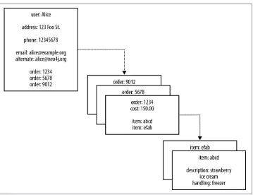
[image:33.504.75.434.231.507.2]When we look at an aggregate store model, such as the one in Figure 2-3, we imagine we can see relationships. Seeing a reference to order: 1234 in the record beginning user: Alice, we infer a connection between user: Alice and order: 1234. This gives us false hope that we can use keys and values to manage graphs.
Figure 2-3. Reifying relationships in an aggregate store
aggregates with structure, in the form of nested maps. Instead, the application that uses the database must build relationships from these flat, disconnected data struc‐ tures. We also have to ensure that the application updates or deletes these foreign aggregate references in tandem with the rest of the data. If this doesn’t happen, the store will accumulate dangling references, which can harm data quality and query performance.
Links and Walking
The Riak key-value store allows each of its stored values to be augmented with link metadata. Each link is one-way, pointing from one stored value to another. Riak allows any number of these links to be walked (in Riak terminology), making the model somewhat connected. However, this link walking is powered by map-reduce, which is relatively latent. Unlike a graph database, this linking is suitable only for sim‐ ple graph-structured programming rather than general graph algorithms.
There’s another weak point in this scheme. Because there are no identifiers that “point” backward (the foreign aggregate “links” are not reflexive, of course), we lose the ability to run other interesting queries on the database. For example, with the structure shown in Figure 2-3, asking the database who has bought a particular prod‐ uct—perhaps for the purpose of making a recommendation based on a customer pro‐ file—is an expensive operation. If we want to answer this kind of question, we will likely end up exporting the dataset and processing it via some external compute infra‐ structure, such as Hadoop, to brute-force compute the result. Alternatively, we can retrospectively insert backward-pointing foreign aggregate references, and then query for the result. Either way, the results will be latent.
It’s tempting to think that aggregate stores are functionally equivalent to graph data‐ bases with respect to connected data. But this is not the case. Aggregate stores do not maintain consistency of connected data, nor do they support what is known as index-free adjacency, whereby elements contain direct links to their neighbors. As a result, for connected data problems, aggregate stores must employ inherently latent methods for creating and querying relationships outside the data model.
Figure 2-4. A small social network encoded in an aggregate store
With this structure, it’s easy to find a user’s immediate friends—assuming, of course, the application has been diligent in ensuring identifiers stored in the friends prop‐ erty are consistent with other record IDs in the database. In this case we simply look up immediate friends by their ID, which requires numerous index lookups (one for each friend) but no brute-force scans of the entire dataset. Doing this, we’d find, for example, that Bob considers Alice and Zach to be friends.
But friendship isn’t always symmetric. What if we’d like to ask “who is friends with Bob?” rather than “who are Bob’s friends?” That’s a more difficult question to answer, and in this case our only option would be to brute-force scan across the whole dataset looking for friends entries that contain Bob.
O-Notation and Brute-Force Processing
We use O-notation as a shorthand way of describing how the performance of an algo‐ rithm changes with the size of the dataset. An O(1) algorithm exhibits constant-time performance; that is, the algorithm takes the same time to execute irrespective of the size of the dataset. An O(n) algorithm exhibits linear performance; when the dataset doubles, the time taken to execute the algorithm doubles. An O(log n) algorithm exhibits logarithmic performance; when the dataset doubles, the time taken to exe‐ cute the algorithm increases by a fixed amount. The relative performance increase may appear costly when a dataset is in its infancy, but it quickly tails off as the dataset gets a lot bigger. An O(m log n) algorithm is the most costly of the ones considered in this book. With an O(m log n) algorithm, when the dataset doubles, the execution time doubles and increments by some additional amount proportional to the number of elements in the dataset.
Brute-force computing an entire dataset is O(n) in terms of complexity because all n
reasonable-sized datasets, where we’d prefer an O(log n) algorithm—which is some‐ what efficient because it discards half the potential workload on each iteration—or better.
Conversely, a graph database provides constant order lookup for the same query. In this case, we simply find the node in the graph that represents Bob, and then follow any incoming friend relationships; these relationships lead to nodes that represent people who consider Bob to be their friend. This is far cheaper than brute-forcing the result because it considers far fewer members of the network; that is, it considers only those that are connected to Bob. Of course, if everybody is friends with Bob, we’ll still end up considering the entire dataset.
To avoid having to process the entire dataset, we could denormalize the storage model by adding backward links. Adding a second property, called perhaps frien ded_by, to each user, we can list the incoming friendship relations associated with that user. But this doesn’t come for free. For starters, we have to pay the initial and ongoing cost of increased write latency, plus the increased disk utilization cost for storing the additional metadata. On top of that, traversing the links remains expen‐ sive, because each hop requires an index lookup. This is because aggregates have no notion of locality, unlike graph databases, which naturally provide index-free adja‐ cency through real—not reified—relationships. By implementing a graph structure atop a nonnative store, we get some of the benefits of partial connectedness, but at substantial cost.
This substantial cost is amplified when it comes to traversing deeper than just one hop. Friends are easy enough, but imagine trying to compute—in real time—friends-of-friends, or friends-of-friends-of-friends. That’s impractical with this kind of data‐ base because traversing a fake relationship isn’t cheap. This not only limits your chances of expanding your social network, it also reduces profitable recommenda‐ tions, misses faulty equipment in your data center, and lets fraudulent purchasing activity slip through the net. Many systems try to maintain the appearance of graph-like processing, but inevitably it’s done in batches and doesn’t provide the real-time interaction that users demand.
Graph Databases Embrace Relationships
The previous examples have dealt with implicitly connected data. As users we infer semantic dependencies between entities, but the data models—and the databases themselves—are blind to these connections. To compensate, our applications must create a network out of the flat, disconnected data at hand, and then deal with any slow queries and latent writes across denormalized stores that arise.
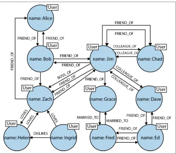
connected data is stored as connected data. Where there are connections in the domain, there are connections in the data. For example, consider the social network shown in Figure 2-5.
Figure 2-5. Easily modeling friends, colleagues, workers, and (unrequited) lovers in a graph
In this social network, as in so many real-world cases of connected data, the connec‐ tions between entities don’t exhibit uniformity across the domain—the domain is variably-structured. A social network is a popular example of a densely connected, variably-structured network, one that resists being captured by a one-size-fits-all schema or conveniently split across disconnected aggregates. Our simple network of friends has grown in size (there are now potential friends up to six degrees away) and expressive richness. The flexibility of the graph model has allowed us to add new
The graph offers a much richer picture of the network. We can see who LOVES whom (and whether that love is requited). We can see who is a COLLEAGUE_OF whom, and who is BOSS_OF them all. We can see who’s off the market, because they’re MARRIED_TO someone else; we can even see the antisocial elements in our otherwise social net‐ work, as represented by DISLIKES relationships. With this graph at our disposal, we can now look at the performance advantages of graph databases when dealing with connected data.
Labels in the Graph
Often we want to categorize the nodes in our networks according to the roles they play. Some nodes, for example, might represent users, whereas others represent orders or products. In Neo4j, we use labels to represent the roles a node plays in the graph. Because a node can fulfill several different roles in a graph, Neo4j allows us to add more than one label to a node.
Using labels in this way, we can group nodes. We can ask the database, for example, to find all the nodes labeled User. (Labels also provide a hook for declaratively indexing nodes, as we shall see later.) We use labels extensively in the examples in the rest of this book. Where a node represents a user, we’ve added a User label; where it repre‐ sents an order we’ve added an Order label, and so on. We’ll explain the syntax in the next chapter.
Relationships in a graph naturally form paths. Querying—or traversing—the graph involves following paths. Because of the fundamentally path-oriented nature of the data model, the majority of path-based graph database operations are highly aligned with the way in which the data is laid out, making them extremely efficient. In their book Neo4j in Action, Partner and Vukotic perform an experiment using both a rela‐ tional store and Neo4j. The comparison shows that the graph database (in this case, Neo4j and its Traversal Framework) is substantially quicker for connected data than a relational store.
Table 2-1. Finding extended friends in a relational database versus efficient finding in Neo4j
Depth RDBMS execution time(s) Neo4j execution time(s) Records returned
2 0.016 0.01 ~2500
3 30.267 0.168 ~110,000
4 1543.505 1.359 ~600,000
5 Unfinished 2.132 ~800,000
At depth two (friends-of-friends), both the relational database and the graph database perform well enough for us to consider using them in an online system. Although the Neo4j query runs in two-thirds the time of the relational one, an end user would barely notice the difference in milliseconds between the two. By the time we reach depth three (friend-of-friend-of-friend), however, it’s clear that the relational database can no longer deal with the query in a reasonable time frame: the 30 seconds it takes to complete would be completely unacceptable for an online system. In contrast, Neo4j’s response time remains relatively flat: just a fraction of a second to perform the query—definitely quick enough for an online system.
At depth four the relational database exhibits crippling latency, making it practically useless for an online system. Neo4j’s timings have deteriorated a little too, but the latency here is at the periphery of being acceptable for a responsive online system. Finally, at depth five, the relational database simply takes too long to complete the query. Neo4j, in contrast, returns a result in around two seconds. At depth five, it turns out that almost the entire network is our friend. Because of this, for many real-world use cases we’d likely trim the results, thereby reducing the timings.
The social network example helps illustrate how different technologies deal with con‐ nected data, but is it a valid use case? Do we really need to find such remote “friends”? Perhaps not. But substitute any other domain for the social network, and you’ll see we experience similar performance, modeling, and maintenance benefits. Whether music or data center management, bio-informatics or football statistics, network sen‐ sors or time-series of trades, graphs provide powerful insight into our data. Let’s look, then, at another contemporary application of graphs: recommending products based on a user’s purchase history and the histories of his friends, neighbors, and other peo‐ ple like him. With this example, we’ll bring together several independent facets of a user’s lifestyle to make accurate and profitable recommendations.
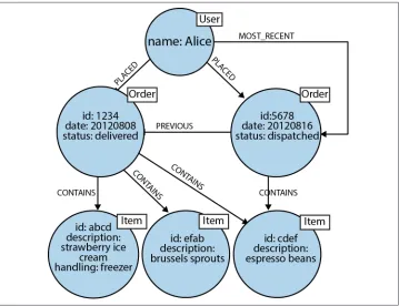
We’ll start by modeling the purchase history of a user as connected data. In a graph, this is as simple as linking the user to her orders, and linking orders together to pro‐ vide a purchase history, as shown in Figure 2-6.
The graph shown in Figure 2-6 provides a great deal of insight into customer behav‐ ior. We can see all the orders a user has PLACED, and we can easily reason about what each order CONTAINS. To this core domain data structure we’ve then added support for several well-known access patterns. For example, users often want to see their order history, so we’ve added a linked list structure to the graph that allows us to find a user’s most recent order by following an outgoing MOST_RECENT relationship. We can then iterate through the list, going further back in time, by following each PREVI OUS relationship. If we want to move forward in time, we can follow each PREVIOUS relationship in the opposite direction, or add a reciprocal NEXT relationship.
1The Neo4j-spatial library conveniently takes care of n-dimensional polygon indexes for us. See https:// github.com/neo4j-contrib/spatial.
Figure 2-6. Modeling a user’s order history in a graph
2For an overview of similarity measures, see Klein, D.J. May 2010. “Centrality measure in graphs.” Journal of Mathematical Chemistry 47(4): 1209-1223.
Such pattern-matching queries are extremely difficult to write in SQL, and laborious to write against aggregate stores, and in both cases they tend to perform very poorly. Graph databases, on the other hand, are optimized for precisely these types of traversals and pattern-matching queries, providing in many cases millisecond responses. Moreover, most graph databases provide a query lan‐ guage suited to expressing graph constructs and graph queries. In the next chapter, we’ll look at Cypher, which is a pattern-matching language tuned to the way we tend to describe graphs using dia‐ grams.
We can use our example graph to make recommendations to users, but we can also use it to benefit the seller. For example, given certain buying patterns (products, cost of typical order, and so on), we can establish whether a particular transaction is potentially fraudulent. Patterns outside of the norm for a given user can easily be detected in a graph and then flagged for further attention (using well-known similar‐ ity measures from the graph data-mining literature), thus reducing the risk for the seller.2
From the data practitioner’s point of view, it’s clear that the graph database is the best technology for dealing with complex, variably structured, densely connected data— that is, with datasets so sophisticated they are unwieldy when treated in any form other than a graph.
Summary
CHAPTER 3
Data Modeling with Graphs
In previous chapters we’ve described the substantial benefits of the graph database when compared both with other NOSQL stores and with traditional relational data‐ bases. But having chosen to adopt a graph database, the question arises: how do we model in graphs?
This chapter focuses on graph modeling. Starting with a recap of the labeled property graph model—the most widely adopted graph data model—we then provide an over‐ view of the graph query language used for most of the code examples in this book: Cypher. Though there are several graph query languages in existence, Cypher is the most widely deployed, making it the de facto standard. It is also easy to learn and understand, especially for those of us coming from a SQL background. With these fundamentals in place, we dive straight into some examples of graph modeling. With our first example, based on a systems management domain, we compare relational and graph modeling techniques. In the second example, the production and con‐ sumption of Shakespearean literature, we use a graph to connect and query several disparate domains. We end the chapter by looking at some common pitfalls when modeling with graphs, and highlight some good practices.
Models and Goals
Graph representations are no different in this respect. What perhaps differentiates them from many other data modeling techniques, however, is the close affinity between the logical and physical models. Relational data management techniques require us to deviate from our natural language representation of the domain: first by cajoling our representation into a logical model, and then by forcing it into a physical model. These transformations introduce semantic dissonance between our conceptu‐ alization of the world and the database’s instantiation of that model. With graph data‐ bases, this gap shrinks considerably.
We Already Communicate in Graphs
Graph modeling naturally fits with the way we tend to abstract details from a domain using circles and boxes, and then describe the connections between these things by joining them with arrows and lines. Today’s graph databases, more than any other database technologies, are “whiteboard friendly.” The typical whiteboard view of a problem is a graph. What we sketch in our creative and analytical modes maps closely to the data model we implement inside the database.
In terms of expressivity, graph databases reduce the impedance mismatch between analysis and implementation that has plagued relational database implementations for many years. What is particularly interesting about such graph models is the fact that they not only communicate how we think things are related, but they also clearly communicate the kinds of questions we want to ask of our domain.
As we’ll see throughout this chapter, graph models and graph queries are really just two sides of the same coin.
The Labeled Property Graph Model
We introduced the labeled property graph model in Chapter 1. To recap, these are its salient features:
• A labeled property graph is made up of nodes, relationships, properties, and labels. • Nodes contain properties. Think of nodes as documents that store properties in
the form of arbitrary key-value pairs. In Neo4j, the keys are strings and the values are the Java string and primitive data types, plus arrays of these types.
• Nodes can be tagged with one or more labels. Labels group nodes together, and indicate the roles they play within the dataset.
1For reference documentation, see http://goo.gl/W7Jh6x and http://goo.gl/ftv8Gx.
• Like nodes, relationships can also have properties. The ability to add properties to relationships is particularly useful for providing additional metadata for graph algorithms, adding additional semantics to relationships (including quality and weight), and for constraining queries at runtime.
These simple primitives are all we need to create sophisticated and semantically rich models. So far, all our models have been in the form of diagrams. Diagrams are great for describing graphs outside of any technology context, but when it comes to using a database, we need some other mechanism for creating, manipulating, and querying data. We need a query language.
Querying Graphs: An Introduction to Cypher
Cypher is an expressive (yet compact) graph database query language. Although cur‐ rently specific to Neo4j, its close affinity with our habit of representing graphs as dia‐ grams makes it ideal for programmatically describing graphs. For this reason, we use Cypher throughout the rest of this book to illustrate graph queries and graph con‐ structions. Cypher is arguably the easiest graph query language to learn, and is a great basis for learning about graphs. Once you understand Cypher, it becomes very easy to branch out and learn other graph query languages.
In the following sections we’ll take a brief tour through Cypher. This isn’t a reference document for Cypher, however—merely a friendly introduction so that we can explore more interesting graph query scenarios later on.1
Other Query Languages
Cypher Philosophy
Cypher is designed to be easily read and understood by developers, database profes‐ sionals, and business stakeholders. Its ease of use derives from the fact that it is in accord with the way we intuitively describe graphs using diagrams.
Cypher enables a user (or an application acting on behalf of a user) to ask the data‐ base to find data that matches a specific pattern. Colloquially, we ask the database to “find things like this.” And the way we describe what “things like this” look like is to draw them, using ASCII art. Figure 3-1 shows an example of a simple pattern.
Figure 3-1. A simple graph pattern, expressed using a diagram
This pattern describes three mutual friends. Here’s the equivalent ASCII art represen‐ tation in Cypher:
(emil)<-[:KNOWS]-(jim)-[:KNOWS]->(ian)-[:KNOWS]->(emil)
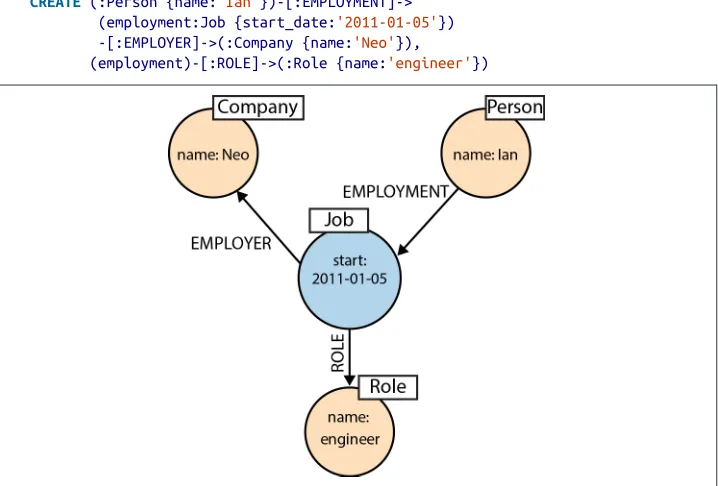
The previous Cypher pattern describes a simple graph structure, but it doesn’t yet refer to any particular data in the database. To bind the pattern to specific nodes and relationships in an existing dataset we must specify some property values and node labels that help locate the relevant elements in the dataset. For example:
(emil:Person {name:'Emil'})
<-[:KNOWS]-(jim:Person {name:'Jim'}) -[:KNOWS]->(ian:Person {name:'Ian'}) -[:KNOWS]->(emil)
Here we’ve bound each node to its identifier using its name prop‐ erty and Person label. The emil identifer, for example, is bound to a node in the dataset with a label Person and a name property whose value is Emil. Anchoring parts of the pattern to real data in this way is normal Cypher practice, as we shall see in the following sections.
Specification by Example
The interesting thing about graph diagrams is that they tend to contain specific instances of nodes and relationships, rather than classes or archetypes. Even very large graphs are typically illustrated using smaller subgraphs made from real nodes and relationships. In other words, we tend to describe graphs using specification by example.
ASCII art graph patterns are fundamental to Cypher. A Cypher query anchors one or more parts of a pattern to specific locations in a graph using predicates, and then flexes the unanchored parts around to find local matches.
The anchor points in the real graph, to which some parts of the pattern are bound, are determined by Cypher based on the labels and property predicates in the query. In most cases, Cypher uses metainformation about existing indexes, constraints, and predi‐ cates to figure things out automatically. Occasionally, however, it helps to specify some additional hints.
Like most query languages, Cypher is composed of clauses. The simplest queries con‐ sist of a MATCH clause followed by a RETURN clause (we’ll describe the other clauses you can use in a Cypher query later in this chapter). Here’s an example of a Cypher query that uses these three clauses to find the mutual friends of a user named Jim:
MATCH (a:Person {name:'Jim'})-[:KNOWS]->(b)-[:KNOWS]->(c), (a)-[:KNOWS]->(c)
Let’s look at each clause in more detail.
MATCH
The MATCH clause is at the heart of most Cypher queries. This is the specification by
example part. Using ASCII characters to represent nodes and relationships, we draw
the data we’re interested in. We draw nodes with parentheses, and relationships using pairs of dashes with greater-than or less-than signs (--> and <--). The < and > signs indicate relationship direction. Between the dashes, set off by square brackets and prefixed by a colon, we put the relationship name. Node labels are similarly prefixed by a colon. Node (and relationship) property key-value pairs are then specified within curly braces (much like a Javascript object).
In our example query, we’re looking for a node labeled Person with a name property whose value is Jim. The return value from this lookup is bound to the identifier a. This identifier allows us to refer to the node that represents Jim throughout the rest of the query.
This start node is part of a simple pattern [:KNOWS]->(b)-[:KNOWS]->(c), (a)-[:KNOWS]->(c) that describes a path comprising three nodes, one of which we’ve bound to the identifier a, the others to b and c. These nodes are connected by way of several KNOWS relationships, as per Figure 3-1.
This pattern could, in theory, occur many times throughout our graph data; with a large user set, there may be many mutual relationships corresponding to this pattern. To localize the query, we need to anchor some part of it to one or more places in the graph. In specifying that we’re looking for a node labeled Person whose name prop‐ erty value is Jim, we’ve bound the pattern to a specific node in the graph—the node representing Jim. Cypher then matches the remainder of the pattern to the graph immediately surrounding this anchor point. As it does so, it discovers nodes to bind to the other identifiers. While a will always be anchored to Jim, b and c will be bound to a sequence of nodes as the query executes.
Alternatively, we can express the anchoring as a predicate in the WHERE clause. MATCH (a:Person)-[:KNOWS]->(b)-[:KNOWS]->(c), (a)-[:KNOWS]->(c)
WHERE a.name = 'Jim' RETURN b, c
Here we’ve moved the property lookup from the MATCH clause to the WHERE clause. The outcome is the same as our earlier query.
RETURN
the nodes bound to the b and c identifiers. Each matching node is lazily bound to its identifier as the client iterates the results.
Other Cypher Clauses
The other clauses we can use in a Cypher query include: WHERE
Provides criteria for filtering pattern matching results. CREATE and CREATE UNIQUE
Create nodes and relationships. MERGE
Ensures that the supplied pattern exists in the graph, either by reusing existing nodes and relationships that match the supplied predicates, or by creating new nodes and relationships.
DELETE
Removes nodes, relationships, and properties. SET
Sets property values. FOREACH
Performs an updating action for each element in a list. UNION
Merges results from two or more queries. WITH
Chains subsequent query parts and forwards results from one to the next. Similar to piping commands in Unix.
START
Specifies one or more explicit starting points—nodes or relationships—in the graph. (START is deprecated in favor of specifying anchor points in a MATCH clause.)
If these clauses look familiar—especially if you’re a SQL developer—that’s great! Cypher is intended to be familiar enough to help you move rapidly along the learning curve. At the same time, it’s different enough to emphasize that we’re dealing with graphs, not relational sets.
Now that we’ve seen how we can describe and query a graph using Cypher, we can look at some examples of graph modeling.
A Comparison of Relational and Graph Modeling
To introduce graph modeling, we’re going to look at how we model a domain using both relational- and graph-based techniques. Most developers and data professionals are familiar with RDBMS (relational database management systems) and the associ‐ ated data modeling techniques; as a result, the comparison will highlight a few simi‐ larities, and many differences. In particular, we’ll see how easy it is to move from a conceptual graph model to a physical graph model, and how little the graph model distorts what we’re trying to represent versus the relational model.
To facilitate this comparison, we’ll examine a simple data center management domain. In this domain, several data centers support many applications on behalf of many customers using different pieces of infrastructure, from virtual machines to physical load balancers. An example of this domain is shown in Figure 3-2.
In Figure 3-2 we see a somewhat simplified view of several applications and the data center infrastructure necessary to support them. The applications, represented by nodes App 1, App 2, and App 3, depend on a cluster of databases labeled Database Server 1, 2, 3. While users logically depend on the availability of an application and its data, there is additional physical infrastructure between the users and the application; this infrastructure includes virtual machines (Virtual Machine 10, 11, 20, 30, 31), real servers (Server 1, 2, 3), racks for the servers (Rack 1, 2 ), and load balancers (Load Balancer 1, 2), which front the apps. In between each of the components there are, of course, many networking elements: cables, switches, patch panels, NICs (network interface controllers), power supplies, air conditioning, and so on—all of which can fail at inconvenient times. To complete the picture we have a straw-man single user of application 3, represented by User 3.
As the operators of such a system, we have two primary concerns:
• Ongoing provision of functionality to meet (or exceed) a service-level agreement, including the ability to perform forward-looking analyses to determine single points of failure, and retrospective analyses to rapidly determine the cause of any customer complaints regarding the availability of service.
Figure 3-2. Simplified snapshot of application deployment within a data center
If we are building a data center management solution, we’ll want to ensure that the underlying data model allows us to store and query data in a way that efficiently addresses these primary concerns. We’ll also want to be able to update the underlying model as the application portfolio changes, the physical layout of the data center evolves, and virtual machine instances migrate. Given these needs and constraints, let’s see how the relational and graph models compare.
Relational Modeling in a Systems Management Domain
and discussions between subject matter experts and systems and data architects. To express our common understanding and agreement, we typically create a diagram such as the one in Figure 3-2, which is a graph.
The next stage captures this agreement in a more rigorous form such as an entity-relationship (E-R) diagram—another graph. This transformation of the conceptual model into a logical model using a stricter notation provides us with a second chance to refine our domain vocabulary so that it can be shared with relational database spe‐ cialists. (Such approaches aren’t always necessary: adept relational users often move directly to table design and normalization without first describing an intermediate E-R diagram.) In our example, we’ve captured the domain in the E-E-R diagram shown in Figure 3-3.
Despite being graphs, E-R diagrams immediately demonstrate the shortcomings of the relational model for capturing a rich domain. Although they allow relationships to be named (something that graph databases fully embrace, but which relational stores do not), E-R diagrams allow only single, undirected, named relationships between entities. In this respect, the relational model is a poor fit for real-world domains where relationships between entities are both numerous and semantically rich and diverse.
Figure 3-3. An entity-relationship diagram for the data center domain
We now have a normalized model that is relatively faithful to the domain. This model, though imbued with substantial accidental complexity in the form of foreign keys and join tables, contains no duplicate data. But our design work is not yet com‐ plete. One of the challenges of the relational paradigm is that normalized models gen‐ erally aren’t fast enough for real-world needs. For many production systems, a normalized schema, which in theory is fit for answering any kind of ad hoc question we may wish to pose to the domain, must in practice be further adapted and special‐ ized for specific access patterns. In other words, to make relational stores perform well enough for regular application needs, we have to abandon any vestiges of true domain affinity and accept that we have to change the user’s data model to suit the database engine, not the user. This technique is called denormalization.
Figure 3-4. Tables and relationships for the data center domain
Although denormalization may be a safe thing to do (assuming developers under‐ stand the denormalized model and how it maps to their domain-centric code, and
have robust transactional support from the database), it is usually not a trivial task. For the best results, we usually turn to a true RDBMS expert to munge our normal‐ ized model into a denormalized one aligned with the characteristics of the underlying RDBMS and physical storage tier. In doing this, we accept that there may be substan‐ tial data redundancy.
The amortized view of data model change, in which costly changes during develop‐ ment are eclipsed by the long-term benefits of a stable model in production, assumes that systems spend the majority of their time in production environments, and that these production environments are stable. Though it may be the case that most sys‐ tems spend most of their time in production environments, these environments are rarely stable. As business requirements change or regulatory requirements evolve, so must our systems and the data structures on which they are built.
Data models invariably undergo substantial revision during the design and develop‐ ment phases of a project, and in almost every case, these revisions are intended to accommodate the model to the needs of the applications that will consume it once it is in production. These initial design influences are so powerful that it becomes nearly impossible to modify the application and the model once they’re in production to accommodate things they were not originally designed to do.
The technical mechanism by which we introduce structural change into a database is called migration, as popularized by application development frameworks such as Rails. Migrations provide a structured, step-wise approach to applying a set of data‐ base refactorings to a database so that it can be responsibly evolved to meet the changing needs of the applications that use it. Unlike code refactorings, however, which we typically accomplish in a matter of seconds or minutes, database refactor‐ ings can take weeks or months to complete, with downtime for schema changes. Database refactoring is slow, risky, and expensive.