The Thirty-Third AAAI Conference on Artificial Intelligence (AAAI-19)
Learning Diverse Bayesian Networks
Cong Chen, Changhe Yuan
Graduate Center and Queens CollegeCity University of New York {cong.chen, changhe.yuan}@qc.cuny.edu
Abstract
Much effort has been directed at developing algorithms for learning optimal Bayesian network structures from data. When given limited or noisy data, however, the optimal Bayesian network often fails to capture the true underlying network structure. One can potentially address the problem by finding multiple most likely Bayesian networks (K-Best) in the hope that one of them recovers the true model. How-ever, it is often the case that some of the best models come from the same peak(s) and are very similar to each other; so they tend to fail together. Moreover, many of these models are not even optimal respective to any causal ordering, thus unlikely to be useful. This paper proposes a novel method for finding a set ofdiversetop Bayesian networks, calledmodes, such that each network is guaranteed to be optimal in a local neighborhood. Such mode networks are expected to provide a much better coverage of the true model. Based on a global-local theorem showing that a mode Bayesian network must be optimal in all local scopes, we introduce an A* search algo-rithm to efficiently find top M Bayesian networks which are highly probable and naturally diverse. Empirical evaluations show that our top mode models have much better diversity as well as accuracy in discovering true underlying models than those found by K-Best.
Introduction
Bayesian networks (BN) (Pearl 1988) are graphical models that represent probabilistic dependencies between random variables. While BNs have become one of the most pop-ular and well-studied probabilistic models, a common bot-tleneck lies in deciding upon their structure. Exactly learn-ing the network structures from the data is known to be NP-hard, even if we restrict each variable to have at most two parents (Chickering 1996). Despite the difficulty of structure learning, a variety of algorithms have been pro-posed to learn optimal Bayesian networks, including dy-namic programming (Koivisto and Sood 2004; Silander and Myllym¨aki 2006), linear programming (Jaakkola et al. 2010; Cussens 2011), and admissible heuristic search (Yuan, Mal-one, and Wu 2011; Yuan and Malone 2013). They all take scores of candidate parent sets of all variables as input, and use various optimization techniques to find a structure that is a good predictor of the data.
Copyright c2019, Association for the Advancement of Artificial Intelligence (www.aaai.org). All rights reserved.
However, even the optimal Bayesian network may fail to capture the true underlying network structure. Such discrep-ancy is called generalization error of the learning problem, which may come from the approximation error, due to the limitations of the models, or estimation error, due to the in-sufficiencies of the data (Bousquet and Bottou 2008). One can potentially address the limitation of the optimal model by finding multiple best Bayesian networks with the highest scores (K-Best) in hope that one of them recovers the true model. It is often the case, however, that some of these top models come from the same peak(s) and are very similar to each other. For example, one of the top solutions may be ob-tained from modifying the best Bayesian network a bit by selecting a slightly worse parent set for one of the variables. Such a solution should not be considered as a top solution for two reasons: (1) it is too similar to another better solu-tion, and (2) it is not even optimal respective to any causal ordering.
In this paper, we propose a novel method for finding a set of diverse top Bayesian networks, called modes, such
that each network is guaranteed to be optimal in a local neighborhood. Such a diverse set of mode models are ex-pected to provide a much better coverage of true underly-ing model. This work is inspired by recent success in devel-oping methods for finding multiple diverse predictions, in-cluding Diverse Best (Batra et al. 2012), joint Diverse M-Best (Kirillov et al. 2015), and M-Modes (Chen et al. 2013; 2018). Based on a global-local theorem showing that a mode Bayesian network must be optimal in all local scopes, we in-troduce an A* search algorithm to efficiently find the top M Bayesian networks which are highly probable and naturally diverse. Empirical evaluations show that our top mode mod-els have much better accuracy in discovering the true causal model than the most likely models found by K-Best.
Bayesian Network Structure Learning
ABayesian networkis a directed acyclic graph (DAG) that
represents the uncertain relations between a set of random variablesV ={v1, . . . , v|V|}. The relations are quantified
using a set of conditional probability distributionsPr vi | pa(vi)
condi-tional probability distributions. We use the terms of variable and vertex interchangeably.
Bayesian network structure learning is the problem of
learning a structure from a complete discrete datasetD =
{d1, . . . , d|D|}, wherediis a data point consisting of values of all variables; each variable takes a value from a finite do-main. Our goal is to find a network structureGthat is a good predictor for the dataD. One of the most popular approaches to this task is score-based learning. Given a network struc-tureG, there is a unique scorescore(G: D)which evalu-ates the goodness of fit ofGto the dataD. For convenience, we will omitD and just usescore(G)instead. The scoring function is typically assumed to be decomposable, that is,
theglobal scorescore(G)can be decomposed into a
summa-tion oflocal scoresas in:score(G) =P
iscorei pa(vi), where the local scorescorei pa(vi)
is the score for each variable vi over its parents pa(vi). Several scoring func-tions have been proposed; most common are the BIC/MDL score (Lam and Bacchus 1994) and the BDe score (Hecker-man, Geiger, and Chickering 1995). Without loss of gener-ality, we assume score is being minimized in the remainder of this paper.
For each variable, the total number of potential parent sets is2|V|−1, the number of subsets of all other variables.
The parent sets of all variables are placed in atable of local
scoresL, with each row containing parent sets of one
vari-able in sorted order. The size of local score tvari-ables can be sig-nificantly reduced by pruning parent sets that are provably non-optimal (Chen, Choi, and Darwiche 2016), that is, these parent sets are never used in any optimal network. Similar to existing research, we also assume that the table of local scores is given as input to our learning problem. How to cal-culate and prune local scores can be found in, e.g., (Campos and Ji 2011).
Given a table of local scores, Bayesian network structure learning becomes a combinatorial optimization problem of selecting one parent set for each variable such that all parent-child relations jointly form a DAG with the minimum score. In particular, if acausal orderingτof variables is provided, there is an optimal Bayesian network that is consistent with this ordering. Each variable can independently choose the best parent set from preceding variables in the ordering.
The complexity of the selection is polynomial inO(|L|). Since each causal ordering maps to a unique optimal score, the goal of learning optimal Bayesian networks is thus to find a causal ordering with the minimum score. There are |V|!different causal orderings. The complexity of a brute
force search of the optimal network isO(|L| · |V|! ).
M-Modes Causal Orderings
We propose toredefinethe problem of finding multiple best
Bayesian networks as finding a set of networks that are not only optimal respective to the best causal orderings but also
diverse. Causal ordering is an inherent property for pruning
worse Bayesian networks; it is especially useful when many local scores are close to each other. Moreover, because of in-sufficiencies in the data, different causal orderings may lead to similar or even the same Bayesian networks. We propose
to only consider top diverse causal orderings that are
lo-cally optimal, that is, they should be better than other causal orderings in its local neighborhood. This is because local swapping of the variables only results in marginally differ-ent models. Instead, we are interested in finding Bayesian network structures that arequalitativelydifferent from each
other.
In this section, we will start by reviewing an ordering-based distance measure called Kendall tau rank distance. We then definemodecausal orderings and prove its global-local
property.
Kendall Tau Rank Distance
The Kendall tau rank distance (Kendall 1938) is a metric that defines the distance between two variable orderings. The larger the distance, the more dissimilar the two orderings are. This distance is defined as counting the total number of discordant pairs for two same length orderings. For exam-ple, there are two same length orderings:τ1=h1,2,3iand
τ2 = h3,1,2i.3 pairs are in these two orderings:h1,2i,
h1,3iandh2,3i. The pairh1,2i’s orders are same in both
orderings, buth1,3iandh1,2iare different. So, in all, the distance is2. It is easy to see that, if two orderings are
iden-tical, the distance will be0, and if one ordering is the reverse of the other, the distance will reach the maximum |τ|
2
, i.e. all pairs of the two orderings are reversed.
M-Modes Orderings
We first define precedence relations between causal order-ings. An orderingτ1precedes another orderingτ2, i.e.τ1≺
τ2, if and only if either (1) the score ofτ1is less thanτ2, or
(2) they have the same score, butτ1is smaller thanτ2in the
lexicographical order. Lexicographical order is used only for breaking ties in a same local neighborhood. We sayτ ≺T when an orderingτ has the highest precedence in the setT (τprecedes all the other orderings in setT).
We use the Kendall tau rank distancekd(·,·)as the
dis-tance metric. Given a non-negative integer δ, called the
scale, theδ-neighborhoodofτ is defined asNδ(τ),{τ0 | kd(τ, τ0)
6δ}, i.e., aδ-neighborhood of an orderingτis a set including all of the orderings which are within distanceδ fromτ. Once ordering precedence andδ-neighborhood are defined, the concepts of local neighborhood and local optima become clear. We define aδ-mode ordering as:
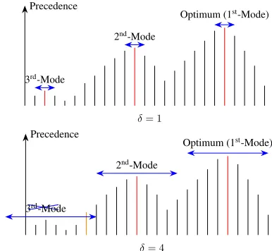
Definition 1(δ-Mode). τis aδ-mode⇔τ ≺ Nδ(τ). Aδ-mode ordering precedes all the other orderings in its δ-neighborhood. This definition ensures that there is only one mode within each givenδ-neighborhood. This also en-sures the set of δ-mode orderings are diverse: any two modes are at least distance δ away. As δ increases, the δ-neighborhood of each τ grows, and the set of δ-modes monotonically shrink until only the global optimum is left:
ˆ
τ ≺ N∞(ˆτ). Theτˆis the global optimal ordering. Figure 1
illustrates what mode solutions andδ-neighborhoods are and how the scaleδaffects the number of modes.
Precedence
δ= 1
Optimum (1st-Mode)
2nd-Mode
3rd-Mode
Precedence
δ= 4
Optimum (1st-Mode)
2nd-Mode
3rd-Mode
Figure 1: An illustration of modes under differentδ. Each vertical bar corresponds to an ordering, and the height cor-responds to its precedence. (Top) When δ = 1, there are
three modes (red). (Bottom) Whenδ = 4, only two modes
are left. The third mode is no longer locally optimal in its δ-neighborhood because of the orange solution.
Problem 1(M-Modes Causal Orderings). Given a scaleδ, compute top M mode causal orderings.
Global-Local Theorem
We cannot rely on Definition 1 in verifying whether a causal ordering is a mode or not, as there are two many causal orderings in itsδ-neighborhood. Inspired by Theorem 2in (Chen et al. 2013) and Theorem1in (Chen, Yuan, and Chen
2016), which show a close connection between the mode la-beling of a graph and the local MAPs of its subgraphs, we present some theoretical properties of a mode causal order-ing and its local patterns.
Consider an example orderingτ = h1,2,3,4,5,6i. We
can create three different orderings with distance 3 via: (a) reverse adjacent variable pairs —h1,2i,h3,4i, andh5,6i — resulting inh2,1,4,3,6,5i; (b) reversingh1,2,3i, re-sulting in h3,2,1,4,5,6i; or (c) moving 1 to between 4
and5, resulting inh2,3,4,1,5,6i. The numbers in
under-line represent thescopeof variables involved in the change.
However, case (a) above can be considered three separate changes in smaller scopes independent from each other, namely, reversing h1,2i, reversing h3,4i, and reversing
h5,6i. We call such a scope of changedivisible. Both case
(b) and case (c) areindivisiblescopes of change. Since the
Kendall tau rank distance is defined as counting reverse pairs, for a given distanceδ, thewidestindivisible scope of
change has a size of at most(δ+ 1), achieved by moving
only one variableδdistance away. Case (c) is an example of that.
The concept ofindivisibilityallows us to exploit the
de-composability of scoring functions. If we can divide a scope of variables into smaller pieces, we only need to verify whether each indivisible scope is optimal. Given an
order-ingτ and a scaleδ, we definelocal ordering,τ[:]as a
con-nected part of τ, where[:] indicates slicing a part fromτ.
The number of variables in a local ordering is itssize. For
example, assuming τ = h4,3,2,1,5,6i,τ[2:4] represents
the local orderingh3,2,1iwith size 3. The example also makes it clear that the orderings with the same distance from an orderingτ can have different sizes of scope. Therefore, given a distanceδ, we further defineδ-scopeof a local
or-dering τ[:] as the set of permutations of the local ordering
which are no more than distanceδfromτ[:]. More formally, scopeδ(τ[:]),{τ[:]0 |kd(τ[:], τ[:]0 )6δ}. The highest
prece-dential local ordering in aδ-scope is called alocal optimum, ˆ
τ[:]. With our previous definition of the precedence rule, a
δ-scope of an ordering must have one and only one local optimum.
Finally, we have the following theorem about a mode or-dering.
Theorem 1(Global-Local). An orderingτ is aδ-Mode if and only if each of its local orderingτ[:] with sizeδ+ 1is optimum in itsδ-scope.
Proof. ⇒(Sufficiency): Supposeτis a mode and∃τ[:]is not
a local optimumτˆ[:]. Bothτ[:]andτˆ[:]have sizeδ+ 1.
Considerτ0is the same asτexcept thatτ0
[:]= ˆτ[:], which
meansτ0goes alongτˆ
[:], so thatτˆ[:]⊆τ0 ∵scopeδ(τ[:]0 ) = scopeδ(τ[:])∴τ0∈ Nδ(τ).
∵τˆ[:]≺τ[:],ˆτ[:]⊆τ0andτ0∈ Nδ(τ)∴τ0 ≺τ. This contradicts the fact thatτis a mode.
⇐(Necessity): Supposeτ is not a mode but∀τ[:] ⊆ τ,
τ[:]= ˆτ[:], which means all of its local orderings are optima,
then∃τ¯∈ Nδ(τ), such thatτ¯is a mode.
Consider τd is the maximal difference between τ and ¯
τ of a scope (means connected). So that, scopeδ(τd) = scopeδ(¯τd). Letτ¯0is the same asτ¯except forτd, such that ˆ
τd⊆¯τ0.
∵ ˆτd ≺τd,τˆd ⊆τ¯0andτ¯0 ∈ Nδ(¯τ) ∴τ¯0 ≺τ. So,¯ τ¯is not a mode.
This contradicts the fact thatτ¯is a mode. So,τmust be a mode.
M-Modes Bayesian Networks
We definemode Bayesian networksto beuniquenetworks
generated from the best mode causal orderings. Different causal orderings may produce the same network structure because there may not be sufficient data to distinguish be-tween these orderings. If these orderings areδdistance away from each other, they are all considered valid mode causal orderings. In practice, we can alleviate, but not solve com-pletely, the problem by increasingδto promote diversity be-tween the orderings, as shown in our empirical results.
We now introduce an A* search algorithm 1 for finding
Algorithm 1Finding M-Modes Bayesian Networks Input: a local scores tableL;δ;M
functionA*-MODE(L,δ,M)
InitializeOpenlist with an empty ordering
whileOpennot emptydo
Pops out the best statecurfromOpen
ifcurfails local-optimum testthenContinue else
ifcuris a complete orderingthen
Extract a mode Bayesian networkbnfromcur
ifbnis unique, andM mode Bayesian networks are foundthenExit elseGenerate successors ofcurand add toOpen
mulate our search space as a tree of all causal orderings. Each node of the search space is called a state which stores an incomplete ordering with a quality score. The root node is the empty ordering. Each node at layerlhasl variables in its partial ordering, and can branch to maximally|V| −l successor nodes. The A* algorithm uses an open list, usually a priority queue, to keep track of frontier states that have not been expanded. At each step, the A* algorithm pops out the
best state from the open list. We subject the current state
to alocal-optimum test. If the test passes, and if the state
is a complete ordering, a mode causal ordering as well as the corresponding mode Bayesian network are found. If the state is not a complete ordering, its successors are generated and added to the open list, called expanding a state. Other-wise if the test fails, the current state will be discarded. Note that because the search space is a tree with no loops, it is un-necessary to have a closed list for duplicate detection. The first few solutions found by A* are guaranteed to be the best mode causal orderings, from which a set of mode Bayesian networks can be extracted. The search continues until we find M unique mode Bayesian networks.
Two aspects of the A* algorithm need further explana-tion. One is the the local-optimum test. The test checks whether all (δ+1)-local orderings of the current state are op-timal in their respectiveδ-scopes. Since the test is done at each search step, only one new (δ+1)-local ordering needs to be checked at any step. Let the best state popped up from the open list represents a partial orderingτ and is at layer l. We only need to check whether it has a local optimum on thetail. We slice the(δ+1)-local orderingτ[l−δ:l] from
τ and enumerate itsδ-scope containing all permutations of the same variables which are no more than distanceδfrom τ[l−δ:l]. If any of the permutation precedesτ[l−δ:l],τfails the
local-optimum test and is discarded. Otherwise,τpasses the test.
For example, ifδ= 2, the open list pops out a state rep-resentingh1,2,3,4i. We check whether the local ordering
h2,3,4iis a local maximum. We enumerate all the mem-bers in itsδ-scope, which contains all permutations except h4,3,2iwhose distance is3. In total we get five permuta-tions to compare with. Ifh2,3,4iprecedes all of the five orderings, it passes the test and is eligible to generate suc-cessor states. Otherwise, stateh1,2,3,4iwill be discarded. The other is thequality scoreof a states,f(s). Thef(s)
is calculated as the sum of a current score,g(s), and a future score,h(s). Theg(s)is the total score from the start state to
s. Theh(s)lower bounds the score fromsto a goal and is estimated from a heuristic function. For Bayesian network learning, g(s)corresponds to the score of the subnetwork over the partial ordering, andh(s)estimates a lower bound
score of the remaining variables. We used the static pattern database-based heuristic function with two random equal-sized groups presented in (Yuan and Maone 2012). The basic idea of the heuristic is to enforce the acyclicity within the predefined groups of variables but relax acyclicity between groups.
The full search tree has up to |V|! leaves and 1 + P|V|
i=1 Qi−1
j=0(|V| −j)nodes. However, because of the
local-optimum test, only mode causal orderings will ever lead to a leave. Also, only one local ordering in theδ-scope of each (δ+1)-local ordering passes the test; all others will end a search branch immediately. Finally, the best-first search strategy of A* only explores the most promising search space in finding the top solutions. The practical search space explored is thus much smaller. Finally, a pseudo code of the A* algorithm is presented in Algorithm 1.
Experiments
We implemented and tested our proposed method (named M-Mode-BNs for short) on top of URLearning2. As
com-monly done in the multiple prediction literature (Batra et al. 2012), we use K-Best as our baseline. In particular, we used theK-Best Software3described in (Tian, He, and Ram
2012). K-Best takes input a complete table of local scores (without pruning) and finds topkbest-scoring networks via a dynamic programming algorithm. K-Best uses the BDe score with a uniform structure prior and an equivalent sam-ple size of1. The same local score tables are used in our M-Mode-BNs method for consistency. Another implicit base-line is M-Mode-BNs method with δ = 0, in which it turns the M best Bayesian networks that are optimal re-spective to any causal ordering. In our experiments, we fo-cus on evaluating exactmethods for solving K-Best or
M-Mode-BNs. Comparing to approximate methods for learn-ing diverse Bayesian networks is interestlearn-ing but left as future
2www.urlearning.org
0 2 4 6 8 10 0
1 2 3 4
M
SHD
K-Best
δ= 0
δ= 1
δ= 3
δ= 5
Figure 2: The average pairwise SHDs for K-Best and M-Mode-BNs on 10 data sets (100data points each) sampled
from Sachs.
work.
We selected several discrete benchmark models from
bnlearn Bayesian Network Repository 4, including
Sur-vey (Scutari and Denis 2014), Asia (Lauritzen and Spiegel-halter 1988), Sachs (Sachs et al. 2005) and Child (Spiegel-halter et al. 1993). Our goal is to test the collective capa-bility of a set of top Bayesian networks in discovering the true underlying causal model, while the goal in (Tian, He, and Ram 2012) was to use top models for Bayesian model averaging. We can also extend our method to perform ap-proximate model averaging, although the extension is left as future work as well.
Our experiments were performed on an IBM System with 32 core 2.67GHz Intel Xeon Processors and 512G RAM. The program was written in C++ using the GNU compiler G++ on a Linux system. We also used functions from an R package calledbnlearnin some data postprocessing tasks.
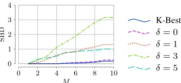
Diversity of Top Models
In the first experiment, we compared the diversity of the top Bayesian networks found by M-Mode-BNs and K-Best. We define thediversityof a set of Bayesian networks as the
av-erage pairwise structural Hamming distance (SHD) between the networks. A larger average SHD means higher diversity. We use the dataset Sachs in this experiment. We randomly sampled 10 data sets with 100 data points each from the network. Then we use our method with differentδ values to learn different numbers of top mode Bayesian networks from each data set. We compared the average diversity of our models against the same numbers of models found by K-Best. Figure 2 shows the results. We can see that mode Bayesian networks found by M-Mode-BNs withδ > 0are
much more diverse than those of K-Best and M-Mode-BNs withδ= 0. In general, largerδresults in higher diversity of learned models, although it is not monotonic. The reason is thatδmeasures the distance between causal orderings, but SHD measures distance between equivalence classes.
Accuracy in Structure Learning
We also compared the ability to recover true models of M-Mode-BNs and K-Best. We use the minimum
struc-tural Hamming distance (SHD) between a set of candidate
4www.bnlearn.com
Bayesian networks and the ground truth network to mea-sure the collective capability of the candidate set in dis-covering the true underlying structure. This is called
or-acle accuracy, i.e., the best one among the top results,
which is commonly used in the literature on multiple di-verse predictions (Batra et al. 2012; Kirillov et al. 2015; Chen et al. 2013).
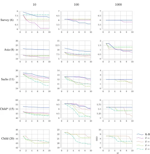
For each benchmark network, we generated three kinds of data sets, with10,100and1000data points respectively; 10 random data sets were sampled for each size and were enough to show the trends. We allow both K-Best and Mode-BNs to find varying numbers of top solutions; M-Mode-BNs with differentδvalues were tested. The average SHD distances over 10 random data sets for all settings are shown in Figure 3. K-Best cannot scale to Child network with20variables, because computing complete local score
tables is extremely expensive for larger data sets. There-fore, we did two experiments on the network. In the first, we dropped5leaf nodes so that we can compare it with K-Best.
In the second, we only ran M-Mode-BNs on the complete Child network with all20variables. M-Mode-BNs is more
scalable than K-Best because it can alternatively take pruned tables of local scores as input.
The results show that M-Mode-BNs withδ > 0in gen-eral has much better oracle accuracies in discovering the true network structures than K-Best. When the data size is small, many network structures receive non-negligible prob-abilities. Many of the top Bayesian networks are structurally quite different from the true underlying structure, because there is simply not enough data to distinguish the models. The average SHD is generally large. When the data size in-creases, there is a dramatic decrease in the average SHD. This means the top Bayesian networks become more simi-lar to the true network. The probability mass also concen-trates more and more on the likely models. K-Best worked better when there are more data. Still, M-Mode-BNs can help to achieve better oracle accuracies in discovering true networks. It is not always predictable whichδ works best for M-Mode-BNs. Our general observation is that the larger theδ, the sparser the top mode Bayesian networks. If there are many mode Bayesian networks, δcan be set higher to achiever better diversity. But ifδis set too high, only very few mode Bayesian networks are left; the accuracy results will suffer as a result. M-Mode-BNs withδ = 0is all over
the map. Sometimes it has the better accuracy results, such as on Survey (10,1000) and Asia (10,1000), but some other
times it is as bad as K-Best, such as on Sachs (100) and Child* (100). It means that simply finding Bayesian
net-works corresponding to best causal orderings cannot reli-ably address the diversity issue of top solutions. We should explicitly promote diversity by using a positiveδ. Note that δis a hyper-parameter whose optimal value depends on spe-cific problems and should be tuned. An optimal δ should reach a balance between both diversity and scores of modes; both of which are necessary for high quality solutions. Fig-ure 3 indicates that the optimalδs are at least correlated with the data set sizes and the network sizes.
10
100
1000
0 2 4 6 8 10
6 6.5 7 7.5 8
Survey (6)
0 2 4 6 8 10
5 5.5 6 6.5 7
0 2 4 6 8 10
5 5.5 6 6.5 7
0 2 4 6 8 10
10 15 20 25 30
Asia (8)
0 2 4 6 8 10
5 7.5 10 12.5 15
0 2 4 6 8 10
0 0.5 1 1.5 2
0 2 4 6 8 10
24 26 28 30
Sachs (11)
0 2 4 6 8 10
10 11 12 13 14
0 2 4 6 8 10
0 1 2 3 4
0 2 4 6 8 10
40 45 50 55 60
Child* (15)
0 2 4 6 8 10
8 8.5 9 9.5 10
0 2 4 6 8 10
5 5.25 5.5 5.75 6
0 2 4 6 8 10
42 43 44 45 46
Child (20)
0 2 4 6 8 10
19 20 21 22 23
0 2 4 6 8 10
6 7 8 9 10
M
SHD
K-Best
δ= 0
δ= 1
δ= 3
δ= 5
10 100 1000
K-Best 6.0/10.0 1.5/10.0 1.0/10.0
δ= 0 6.7/10.0 1.4/10.0 1.0/10.0
δ= 1 8.2/10.0 3.3/10.0 1.5/10.0
δ= 3 9.4/10.0 6.1/9.9 1.8/9.5
δ= 5 8.8/9.3 2.5/4.7 2.2/5.3
Table 1: The average numbers of unique equivalence classes/ top models found by K-Best and M-Mode-BNs for data sets with different sizes on Sachs.
Survey (100) and Asia (1000). On Survey (10),
M-Mode-BNs withδ= 5only found one mode Bayesian network; all other likely Bayesian networks are suppressed because of the largeδ. Similarly on Survey (100) and Asia (1000), the number of data points is large relative to the network size. Again M-Mode-BNs only found very few mode Bayesian networks. In comparison, K-Best often has many more top models to use.
One observation of the results may seem puzzling. Intu-itively, the very best solution should be the same for both K-Best and M-Mode-BNs. Therefore, the accuracy curves of all methods should have the same starting point (when M = 1). However, in some of the graphs, K-Best has worse starting accuracies. Upon further investigations into the re-sults, we found that, although K-Best and M-Mode-BNs al-ways found top models with the same best score, the mod-els may come from different equivalence classes, especially when the amount of data is limited. Therefore, the SHD of the top models found by K-Best and M-Mode-BNs may be different. For some unknown reason, M-Mode-BNs found top models with smaller SHD than K-Best in most cases, but not always.
As mentioned earlier, M-Mode-BNs is much more scal-able than K-Best because it can alternatively take pruned local score tables as input. However, we can see that there are no results for M-Mode-BNs withδ= 0on Child* (15, 1000) or on Child (20). It is because, whenδ = 0, we are essentially performing exhaustive search in the search tree. Whenδis too large, M-Mode-BNs can become less efficient because the local-mode test at each search step is very ex-pensive. Otherwise, M-Mode-BNs with medium or smallδ values tend to have similar efficiency as K-Best. As a typical example, K-Best took 9.5s on average on10random datasets of Child*(15,100) to find the top10 networks, while
M-Mode-BNs took 10.1s whenδ = 1, 5.2s whenδ = 3, and
177s whenδ= 5.
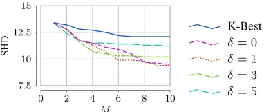
Effect of Equivalence Classes
In Figure 2, the initial diversity stays at 0.0 untilM = 4.
Also in Figure 3, the SHD curves of K-Best often stay flat. This is because many top Bayesian networks found by K-Best are from the same equivalence class and lack diver-sity. As an example, we computed the number of different equivalent classes out of the top solutions for each setting on Sachs and present the results in Table 1. Again, we observe that a largerδoften leads to fewer mode Bayesian networks,
0 2 4 6 8 10
7.5 10 12.5 15
M
SHD
K-Best
δ= 0
δ= 1
δ= 3
δ= 5
Figure 4: The average SHD accuracy for unique equivalence classes found by K-Best and M-Mode-BNs on data sets (100
data points each) sampled from Sachs.
although they tend to be from different equivalence classes. Addressing such diversity issue was the main motivation for us to develop the M-Mode-BNs method. Nevertheless, it is a fair question to ask whether finding top equivalence
classes(Chen and Tian 2014) instead of top Bayesian
net-works can similarly address the diversity issue. In order to obtain some initial insights, we allowed both K-Best and M-Mode-BNs to find as many top models as possible, during which we filtered out models that belong to the same equiv-alence classes of existing models. In other words, we only keep top models that belong to unique equivalence classes. We then compare the oracle accuracies of those filtered mod-els. The results are shown in Figure 4. The results show that the equivalence classes found by M-Mode-BNs still have better oracle accuracies than those of K-Best. The results in-dicate that diversity in equivalence classes is also desirable.
Concluding Remarks
In this paper, we introduce a novel method called M-Mode-BNs for finding a diverse set of top mode Bayesian works. Our results show that the top mode Bayesian net-works found by M-Mode-BNs have much better oracle accu-racies in discovering the true underlying network structures in comparison to K-Best, which simply finds the top mod-els with the best scores. Preliminary results also show that such diversity cannot be achieved by learning top equiva-lence classes. Also, we only used oracle accuracy to eval-uate the quality of mode solutions. In practice, we can ask an expert to choose a final solution (Flerova, Marinescu, and Dechter 2016), rank and combine a very large pool (Li, Car-reira, and Sminchisescu 2010), or even further improve the solutions in a human-in-the-loop environment.
As future work, we plan to generalize our method to find top diverse equivalence classes. Open questions include how to define mode equivalence classes and how to efficiently search for them. We also want to extend our method to per-form approximate model averaging and compare to approx-imate methods for finding diverse Bayesian networks, such as sampling and local search.
Acknowledgment
References
Batra, D.; Yadollahpour, P.; Guzman-Rivera, A.; and Shakhnarovich, G. 2012. Diverse M-best solutions in markov random fields.Computer Vision–ECCV 20121–16.
Bousquet, O., and Bottou, L. 2008. The tradeoffs of large scale learning. In Platt, J. C.; Koller, D.; Singer, Y.; and Roweis, S. T., eds., Advances in Neural Information
Pro-cessing Systems 20. Curran Associates, Inc. 161–168.
Campos, C. P. d., and Ji, Q. 2011. Efficient structure learning of bayesian networks using constraints.Journal of Machine
Learning Research12(Mar):663–689.
Chen, Y., and Tian, J. 2014. Finding the k-best equivalence classes of bayesian network structures for model averaging. InAAAI, 2431–2438.
Chen, C.; Kolmogorov, V.; Zhu, Y.; Metaxas, D.; and Lam-pert, C. H. 2013. Computing the M most probable modes of a graphical model. In International Conf. on Artificial Intelligence and Statistics (AISTATS).
Chen, C.; Yuan, C.; Ye, Z.; and Chen, C. 2018. Solving m-modes in loopy graphs using tree decompositions. In
In-ternational Conference on Probabilistic Graphical Models,
145–156.
Chen, E. Y.-J.; Choi, A.; and Darwiche, A. 2016. On pruning with the mdl score. InConference on Probabilistic
Graphi-cal Models, 98–109.
Chen, C.; Yuan, C.; and Chen, C. 2016. Solving m-modes using heuristic search. InProceedings of the 25th Interna-tional Joint Conference on Artificial Intelligence (IJCAI-16).
Chickering, D. M. 1996. Learning bayesian networks is np-complete. InLearning from data. Springer. 121–130.
Cussens, J. 2011. Bayesian network learning with cutting planes. InProceedings of the Twenty-Seventh Conference on Uncertainty in Artificial Intelligence, 153–160. AUAI Press.
Flerova, N.; Marinescu, R.; and Dechter, R. 2016. Search-ing for the m best solutions in graphical models. Journal of
Artificial Intelligence Research55:889–952.
Heckerman, D.; Geiger, D.; and Chickering, D. M. 1995. Learning bayesian networks: The combination of knowledge and statistical data. Machine learning20(3):197–243.
Jaakkola, T.; Sontag, D.; Globerson, A.; and Meila, M. 2010. Learning bayesian network structure using lp relaxations. In
Proceedings of the Thirteenth International Conference on Artificial Intelligence and Statistics, 358–365.
Kendall, M. G. 1938. A new measure of rank correlation.
Biometrika30(1/2):81–93.
Kirillov, A.; Savchynskyy, B.; Schlesinger, D.; Vetrov, D.; and Rother, C. 2015. Inferring M-Best diverse labelings in a single one. InIEEE International Conference on Computer
Vision (ICCV). IEEE.
Koivisto, M., and Sood, K. 2004. Exact bayesian structure discovery in bayesian networks.Journal of Machine
Learn-ing Research5(May):549–573.
Lam, W., and Bacchus, F. 1994. Learning bayesian belief networks: An approach based on the mdl principle. Compu-tational intelligence10(3):269–293.
Lauritzen, S. L., and Spiegelhalter, D. J. 1988. Local com-putations with probabilities on graphical structures and their application to expert systems. Journal of the Royal
Statisti-cal Society. Series B (MethodologiStatisti-cal)157–224.
Li, F.; Carreira, J.; and Sminchisescu, C. 2010. Object recognition as ranking holistic figure-ground hypotheses.
InComputer Vision and Pattern Recognition (CVPR), 2010
IEEE Conference on, 1712–1719. IEEE.
Pearl, J. 1988. Probabilistic Reasoning in Intelligent
Sys-tems: Networks of Plausible Inference. San Mateo, CA:
Morgan Kaufmann Publishers, Inc.
Sachs, K.; Perez, O.; Pe’er, D.; Lauffenburger, D. A.; and Nolan, G. P. 2005. Causal protein-signaling net-works derived from multiparameter single-cell data.Science
308(5721):523–529.
Scutari, M., and Denis, J.-B. 2014.Bayesian networks: with
examples in R. CRC press.
Silander, T., and Myllym¨aki, P. 2006. A simple approach for finding the globally optimal bayesian network structure.
InProceedings of the Twenty-Second Conference on
Uncer-tainty in Artificial Intelligence, 445–452. AUAI Press.
Spiegelhalter, D. J.; Dawid, A. P.; Lauritzen, S. L.; and Cow-ell, R. G. 1993. Bayesian analysis in expert systems.
Statis-tical science219–247.
Tian, J.; He, R.; and Ram, L. 2012. Bayesian model aver-aging using the k-best bayesian network structures. arXiv preprint arXiv:1203.3520.
Yuan, C., and Malone, B. 2013. Learning optimal Bayesian networks: A shortest path perspective. Journal of Artificial
Intelligence Research (JAIR)48:23–65.
Yuan, C., and Maone, B. 2012. An improved admissible heuristic for learning optimal bayesian networks. In Pro-ceedings of The 28th Conference on Uncertainty in Artificial Intelligence (UAI-12).
Yuan, C.; Malone, B.; and Wu, X. 2011. Learning optimal bayesian networks using A* search. InIJCAI proceedings-international joint conference on artificial intelligence,