Volume 2, Issue 2, February 2013
Page 33
ABSTRACT
In this paper, an inventory model is developed by considering simultaneously the phenomena with two-warehouse, varying rate of deterioration, time dependent demand and variable holding cost. A numerical example and sensitivity analysis on some parameters are implemented to illustrate the model.
1. I
NTRODUCTIONIn the busy markets like super market, municipality market etc. the storage area of items is limited. When an attractive price discount for bulk purchase is available or the cost of procuring goods is higher than the other inventory related cost or demand of items is very high or there are some problems in frequent procurement, management decide to purchase a large amount of items at a time. These items cannot be accommodated in the existing store house (viz. the Own Warehouse, OW) located at busy market place. In this situation, for storing the excess items, one additional warehouse (viz. rented warehouse, RW) is hired on rental basis, which may be located little away from it. We assume that the rent (hold cost for the item) in RW is greater than OW and hence the items are stored first in OW and only excess stock is stored in RW, which are emptied first by transporting the stocks from RW to OW in a continuous release pattern for deducing the holding cost. The demand of items is met up at OW only.
An early discussion on the effect of two warehouses was considered by Hartely (1976),recently this type of inventory model has been considered by other authors. Sarma (1983) developed a deterministic inventory model with finite replenishment rate; Dave (1988) further discussed the cases of bulk release pattern for both finite and infinite replenishments. In the above literature, deterioration phenomenon was not taken into account. Assuming the deterioration in both warehouses, Sarma (1987), extended his earlier model to the case of infinite replenishment rate with shortages. Pakkala and Achary (1992) extended the two-warehouse inventory model for deteriorating items with finite replenishment rate and shortages, taking time as discrete and continuous variable, respectively. In these models mentioned above the demand rate was assumed to be constant. Subsequently, the ideas of time varying demand and stock dependent demand considered by some authors, such as Goswami and Chaudhary (1998), Bhunia and Maiti (1998), Bankerouf (1997), Kar et al. (2001) and others. Bhunia and Maiti (1994) extended the model of Goswami and Chaudhary (1972), in that model they were not consider the deterioration and shortages were allowed and backlogged. Yang (2004) provided a two-warehouse inventory model for a single item with constant demand and shortages under inflation. Zhou and Yang (2005) studied stock-dependent demand without shortage and deterioration with quantity based transportation cost, Wee, Yuond Law (2005) considered a two-warehouse model with constant demand and weibull distribution deterioration under inflation. Yang (2006) extended Yang (2004) to incorporate partial backlogging and then compared the two-warehouse models based on the minimum cost approach.
Most researchers on inventory models do not considered simultaneously the phenomena with two-warehouse, varying rate of deterioration, time dependent demand and variable holding cost. Since these phenomena are not uncommon in real life, we incorporate them in our problem development. A numerical example and sensitivity analysis on some parameters are implemented to illustrate the model.
TWO-WAREHOUSE INVENTORY MODEL
WITH TIME DEPENDENT DEMAND AND
VARIABLE HOLDING COST
Dr. Meghna Tyagi1, Dr. S. R. Singh2
1
Assistant Professor, Department of Applied Sciences, NITRA Technical Campus, Ghaziabad
2
Volume 2, Issue 2, February 2013
Page 34
2. ASSUMPTIONS
AND
NOTATIONS
ASSUMPTIONS :
(i) The demand rate function D(t) is deterministic and is a known function given by D(t) = (
a
bt
), where a, b are positive constants.(ii) The own warehouse (OW) has a fixed capacity of W units; the rented warehouse (RW) has unlimited capacity. (iii)Deterioration of the item follows a two-parameter Weibull distribution.
(iv)There is no replacement or repair of deteriorating items during the period under consideration. (v) Shortages are not allowed and the lead time is zero.
(vi)Holding costs
C
OW(t)
andC
RW(t)
per item per unit time are independent and are assumed in OW and RW respectively asC
OW(t)
C
OW
t
andC
RW(t)
C
RW
t
, where 0<
<1 and 0<
<1.(vii)The RW is located near the OW and thus the transportation cost between them is negligible.
(viii)The inventory cost (including holding cost and deteriorating cost) in RW is higher than that in OW.
NOTATIONS
The following notations are used throughout the paper: P Production rate (units/unit time)
H Planning horizon W Fix storage capacity
Scale parameter of the deterioration rate in OW
Shape parameter of the deterioration rate in OW g Scale parameter of the deterioration rate in RW,
>g h Shape parameter of the deterioration rate in RW1
L
a category of production cycle that only OW is used within the cycle
2
L
a category of production cycle that both OW and RW are used within the cycle n number of production cycles during the entire horizon
0
i
t
the time at the beginning of the ith production cycle belonging to
L
21
i
t
the time at which the inventory level in OW first reaches W units within the production cycle
2
i
t
the time at the end of production of the ith production cycle
3
i
t
the time at which all inventory units in RW are depleted within the ith production cycle
0
j
t
the time at the beginning of the ith production cycle belonging to
L
11
j
t
the time at the end of production for the jth production cycle
1
i
I
inventory level in OW at time t with t
[t , t ]
i0 i12
i
I
Volume 2, Issue 2, February 2013
Page 35
3
i
I
inventory level in RW at time t with t
[t , t ]
i2 i34
i
I
inventory level in OW at time t with t
[t , t
i3 i 1,0]
5
i
I
inventory level in OW at time t with t
[t , t ]
i1 i31
j
I
inventory level in OW at time t with t
[t , t ]
j0 j12
j
I
inventory level in OW at time t with t
[t , t
j1 j 1,0]
i
D
the quantity of deteriorated items during the ith production cycle
j
D
the quantity of deteriorated items during the jth production cycle
j
U
the maximum inventory items during the jth production cycle
1
C
set-up cost per scheduling period
2
C
cost of deteriorated unit
OW
C
holding cost per inventory unit held in OW per unit time
RW
C
holding cost per inventory unit held in RW per unit time TC total system cost during the entire horizon H
3. M
ATHEMATICALM
ODELUsing above assumptions, the inventory level in a production system with time dependent demand and holding cost for deteriorating items is depicted in Fig.1. Fig. 1(a) shows the inventory level during a production cycle in which both OW and RW are used. Within any arbitrary production cycle i belonging to
L
2 the cycle starts fromt
i0 and endsat
t
i 1,0 . During the period of [t , t
i0 i 1,0 ], five points of time are identified in sequence, namelyt , t , t , t
i0 i1 i2 i3and
t
i 1,0 . At 0i
t
production, demand, and deterioration occur simultaneously. Items accumulate from 0 up to W units in OW during the period [0 1
i i
t , t
]. After 1i
t
, any production quantity exceeding W will be stored in RW. The inventory level in RW begins to decrease at2
i
t
and will reach 0 units at 3i
t
because of demand and deterioration. The inventory level in OW comes to decrease at1
i
t
and then falls below W at 3i
t
due to deterioration. The remaining stocks in OW will be fully exhausted att
i 1,0 owing to demand and deterioration.Fig. 1(b) depicts the inventory level during a production cycle in which only OW is used. Within any arbitrary cycle j belonging to
L
1, the inventory behavior can be considered according to two time intervals, [t , t
j0 j1] and [t , t
j1 j 1,0 ].During [
t , t
j0 j1], the inventory level in OW gradually increases but it is always less than W. During [t , t
j1 j 1,0 ], thestocks in OW gradually decreases due to demand and deterioration and will be exhausted at
t
j 1,0 .Volume 2, Issue 2, February 2013
Page 36
Fig. 1: Inventory level in a production system for deteriorating items with Time dependent demand
Given production cycle i belonging to
L
2, the differential equations stating the inventory levels within the cycle are given as follows:1 i1
i1 i0 i1
dI (t)
t I P (a bt), t t t
dt
(1)
h 1 i 2
i2 i1 i 2
dI (t)
ght I P (a bt), t t t
dt
(2) i3 h 1 i3
dI (t)
ght I (a bt), dt
ti 2 t ti3 (3)
1 i4
i4 dI (t)
t I (a bt), dt
t
i3
t
t
i 1,0 (4)1 i5
i5 dI (t)
t I 0, dt
ti1 t ti3 (5)
With the total system cost consists of setup cost, carrying cost, and deteriorating cost incurred in each production cycle within the planning horizon H and can be expressed as
1 RW ,i OW,i
i i
TC = nC
I
I OW, j 2 i 2 jj i j
I C D C D
(6)Case 1.No deterioration in inventory: When deterioration phenomenon does not exist in both warehouses, ie, both α ,
β and g , h approach to zero. The cost in (6) can be rewritten as
1 RW ,i OW,i OW, j
g ,h 0 , 0 , 0
i i i
TC = nC lim I lim I lim I
(7)which states the total cost of two-warehouse inventory for non-deteriorating items.
Case 2. Inventory model for non-deteriorating items with constant demand and time dependent holding cost:
When time dependent demand, and deterioration do not exist in both warehouses, i.e. α, β, g, h and b approach to
zero,
The total cost in (6) can be reduced to
1 g,h 0 RW,i , 0 OW ,i , 0 OW , j i b,c 0 i b,c 0 i b,c 0 TC = nC lim I lim I lim I
(8)
2 22
i 2 i1
1 RW i 2 i1 i1
i
t t
nC C P a t t t
2 2
2 22 i3 i 2
i3 i 3 i 2
t t
a t t t
2 2
3 2 3 3 3 3 2 3
i3 i3
i 2 i 2 i1 i1 i 2 i 2
i1 i3
t t
t t t t t t
(P a) t a t
3 2 3 2 2 3 2 3
2 2 2 i 0 i1
OW i1 i 0 i0
i
t t
C (P a) t t t
2 2
2 2 i 1,0 2 i3i 1,0 i 1,0 i3 i3 i1
t t
a t t t W(t t )
2 2
3 3 3 2i0 i 0 i1 i1
i 0
t t t t
P a t
3 2 3 2
3 3 2 3 2 2
i 1,0 i 1,0 i3 i3 i3 i1
i 1,0
t t t t t t
a t W
2 3 2 3 2 2
2 2
j1 j0 2
OW j1 j0 j0
j
t t
C (P a) t t t
2 2
2 2j 1,0 j1
2
j 1,0 j1 j 1,0
t t
a t t t
2 2
3 2 3 3 3 3 2 3
j1 j1 j0 j0 j 1,0 j 1,0 j1 j1
j0 j 1,0
t t t t t t t t
(P a) t a t
3 2 3 2 2 3 2 3
which is the total system cost for the non-deteriorating items with constant demand and time dependent holding cost. Some important cases of the general model can be further analyzed.
Solution Procedure: As it is quite clear from the model, TC (total cost) is a function of
t
i 0 (initial time of the ith
Volume 2, Issue 2, February 2013
Page 37
i0
TC
0
t
This equation is highly non-linear hence is solved with the help of mathematical software MATHEMATICA 5.2. The equation is solved for different parameters for fixed planning horizon H.
Numerical Example: 1
Optimal production policy to minimize the total system cost may be obtained by using the methodology in the following preceding sections. To illustrate the proposed two warehouse inventory model, following input data is considered: Input Data: Planning Horizon (H) =10,
Production rate (P) = 1800,
Set-up cost (
C
1) = $2500 per setup, OW capacity W = 300 units, Demand (a) = 800,Holding cost in OW (
C
OW) =$5, Holding cost in RW (C
RW) =$8,
=0.3,
=0.5, n=1With the above values we obtained the optimum result
t
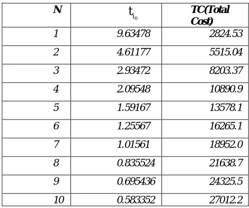
i 0(initial time of the ith production cycle) = 9.63478 and TC (Total cost) =2824.53Table 1: Sensitivity analysis for varying values of N
Table 2: Sensitivity analysis for varying values of P
N P
0
i
t
TC(Total Cost)1 1800 9.63478 2824.53
1 1900 9.64963 2811.44
1 2000 9.66199 2800.53
1 2100 9.67245 2791.30
1 2200 9.68142 2783.39
1 2300 9.68918 2776.53
1 2400 9.69597 2770.53
1 2500 9.70196 2765.23
N
0
i
t
TC(Total Cost)1 9.63478 2824.53
2 4.61177 5515.04
3 2.93472 8203.37
4 2.09548 10890.9
5 1.59167 13578.1
6 1.25567 16265.1
7 1.01561 18952.0
8 0.835524 21638.7
9 0.695436 24325.5
Volume 2, Issue 2, February 2013
Page 38
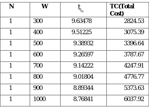
Table 3: Sensitivity analysis for varying values of W
N W
0
i
t
TC(TotalCost)
1 300 9.63478 2824.53
1 400 9.51225 3075.39
1 500 9.38932 3396.64
1 600 9.26597 3787.67
1 700 9.14222 4247.91
1 800 9.01804 4776.77
1 900 8.89344 5373.63
1 1000 8.76841 6037.92
Table 4: Sensitivity analysis for varying values of A
N A
0
i
t
TC(Total Cost)1 800 9.63478 2824.53
1 700 9.62054 2836.85
1 600 9.59411 2859.78
1 500 9.55024 2897.79
1 400 9.47760 2960.42
1 300 9.34908 3070.25
1 200 9.08214 3294.21
1 100 8.25684 3951.21
Table 5: Sensitivity analysis for varying values of
C
RWN
RW
C
0
i
t
TC(Total Cost)1 8 9.63478 2824.53
1 9 9.61240 2844.31
1 10 9.59302 2861.43
1 11 9.57607 2876.38
1 12 9.56112 2889.56
1 13 9.54785 2901.25
1 14 9.53598 2911.70
1 15 9.52531 2921.09
Volume 2, Issue 2, February 2013
Page 39
N
OW
C
0
i
t
TC(Total Cost)1 3 9.63478 2824.53
1 2 9.58217 2808.32
1 1 9.52940 2776.31
1 0.9 9.52411 2772.24
1 0.8 9.51882 2768.01
1 0.7 9.51353 2763.62
1 0.6 9.50824 2759.07
1 0.5 9.50294 2754.36
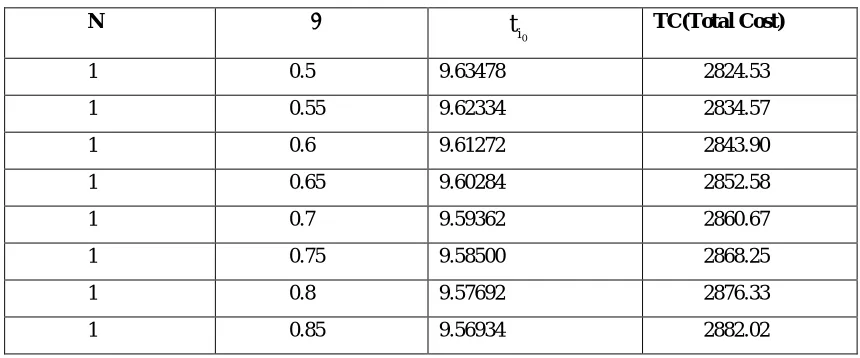
Table 7: Sensitivity analysis for varying values of
N
0
i
t
TC(Total Cost)1 0.5 9.63478 2824.53
1 0.55 9.62334 2834.57
1 0.6 9.61272 2843.90
1 0.65 9.60284 2852.58
1 0.7 9.59362 2860.67
1 0.75 9.58500 2868.25
1 0.8 9.57692 2876.33
1 0.85 9.56934 2882.02
Table 8: Sensitivity analysis for varying values of
N
i 0
t
TC(TotalCost)
1 0.3 9.63478 2824.53
1 0.31 9.63992 2825.27
1 0.32 9.64507 2825.87
1 0.33 9.65022 2826.31
1 0.34 9.65537 2826.60
1 0.35 9.66053 2826.74
1 0.36 9.66569 2826.73
1 0.37 9.67085 2826.57
The main conclusions drawn from the numericalstudy as well as sensitivity analysis are as follows:
From Table 1, it is observed that as the number of cycle’s increases, the total system cost is increasing and
i 0
Volume 2, Issue 2, February 2013
Page 40
For fixed number of cycle i.e. n = 1, when production units increases, the initial time of ith production cycle is increasing and total system cost is decreasing.
In the Table 3, lower rate of demand decreased the
t
i 0 and increased the total cost for n = 1. Increasing storage capacity of own warehouse (W) increased the total cost while decreased
t
i 0(initial time of ith production cycle). From Table 5, for fixed number of cycle i.e. n = 1 increasing holding cost of RW increased the total cost with decreasing
t
i 0. It is assumed for one cycle, decreasing holding cost of OW decreases the time
t
i 0 and corresponding decreasing total cost. From Table 7, n = 1, increasing values of
increased the total cost while decreasingt
i 0. Increasing values of
shows the almost stable total system cost with increasing values oft
i 0(initial time of ith production cycle).4. CONCLUSION
In the present chapter, a two warehouse production inventory model is developed for the deteriorating items. This model incorporates some realistic features that are likely to be associated with some kinds of inventory. The principle features of the model are as follows:
The traditional parameters of holding cost is assumed here to be time varying. As the change in the time value of money and in the price index, holding cost cannot remain constant over time. It is assumed that the holding cost is linearly increasing functions of time.
The two warehouse inventory control is an intriguing yet practicable issue of decision science when time-dependent demand is involved. This problem is different from that with constant demand where keeping a consistent inventory level in the rented warehouse is the best solution.
The variable deterioration factor has been taken into consideration in the present model as almost all items undergo either direct spoilage (like fruits, vegetables etc.) or physical decay (in case of radioactive substances, volatile liquids etc) in the course of time, deterioration is a very natural phenomenon in inventory system. There are many items like perfumes, photographic films etc. which incur a gradual loss of potential or quality over time. A numerical example and sensitivity analysis are implemented to illustrate the model. The present analysis can be
applied for seasonable/fashionable goods which are marketed for a fixed time period. Hence, from the economical point of view, the proposed model will be useful to the business houses in the present context as it gives better inventory control system.
R
EFERENCES:
[1] R.V. Hartley (1976), Operations Research—A Managerial Emphasis, Good Year Publishing Company, California, 315-317.
[2] K.V.S. Sarna (1983), A deterministic inventory model with two level of storage and an optimum release rule, Opsearch 20, 175-180.
[3] T.A. Murdeshwar, Y.S. Sathe (1985), Some aspects of lot size model with two levels of storage, Opsearch 22, 255-262.
[4] U. Dave (1988), On the EOQ models with two levels of storage, Opsearch 25 (1988) 190-196.
[5] K.V.S. Sarma (1987), A deterministic order level inventory model for deteriorating items with two storage facilities. European Journal of Operational Research 29,70-73.
[6] T.P.M. Pakkala, K.K. Achary (1992), Discrete time inventory model for deteriorating items with two- warehouses, Opsearch 29, 90-103.
[7] T.P.M. Pakkala, K.K. Achary (1992), A deterministic inventory model for deteriorating items with two- warehouses and finite replenishment rate, European Journal of Operational Research 57, 157- 167.
Volume 2, Issue 2, February 2013
Page 41
[9] A.K. Bhunia, M. Maiti (1998), A two-warehouse inventory model for deteriorating items with a linear trend in demand and shortages, Journal of the Operational Research Society 49, 287-292.
[10]S. Kar. A.K. Bhunia, M. Maiti (2001), Deterministic inventory model with two levels of storage, a linear trend in demand and a fixed time horizon. Computers & Operations Research 28 , 1315-1331.
[11]Y.W. Zhou (2003), A multi-warehouse inventory model for items with time-varying demand and shortages, Computers & Operations Research 30 , 2115-2134.
[12]A. K. Bhunia and M. Maiti (1994), A two warehouse inventory model for a linear trend in demand, Opsearch 31 [13]J.A. Buzacott (1975), Economic order quantities with inflation, Operational Research Quarterly 26,553- 558. [14]R. B. Misra (1979), A note on optimal inventory management with inflation, Naval Research Logistics
26,161-165.
[15]J. Ray, K. S. Chaudhuri (1997), An EOQ model with stock-dependent demand, shortage, inflation and time discounting, International Journal of Production Economics 53 ,171-180.
AUTHOR
Meghna Tyagi has done M.Sc. in Mathematics and PhD in “Inventory Modelling”. She has over 8 years