Accelerating Cross-Validation in Multinomial Logistic Regression with $\ell_1$-Regularization

(1)

Accelerating Cross-Validation in

Multinomial Logistic Regression with

`

1

-Regularization

Tomoyuki Obuchi [email protected]

Yoshiyuki Kabashima [email protected]

Department of Mathematical and Computing Science Tokyo Institute of Technology

2-12-1, Ookayama, Meguro-ku, Tokyo, Japan

Editor:Manfred Opper

Abstract

We develop an approximate formula for evaluating a cross-validation estimator of predictive likelihood for multinomial logistic regression regularized by an`1-norm. This allows us to avoid repeated optimizations required for literally conducting cross-validation; hence, the computational time can be significantly reduced. The formula is derived through a pertur-bative approach employing the largeness of the data size and the model dimensionality. An extension to the elastic net regularization is also addressed. The usefulness of the approx-imate formula is demonstrated on simulated data and the ISOLET dataset from the UCI machine learning repository. MATLAB and python codes implementing the approximate formula are distributed in (Obuchi, 2017; Takahashi and Obuchi, 2017).

Keywords: classification, multinomial logistic regression, cross-validation, linear pertur-bation, self-averaging approximation

1. Introduction

Multinomial classification is a ubiquitous task. There are several ways to treat this task, such as the naive Bayesian methods, neural networks, decision trees, and hierarchical classi-fication schemes (Trevor et al., 2009). Among them, in this paper, we focus on multinomial logistic regression (MLR), which is simple but powerful enough to be used in many present day applications.

Let us denote each feature vector by xµ ∈RN and its class byyµ ∈ {1,· · · , L}, where

µ = 1· · · , M denotes the index of given data. The MLR uses a linear structural model with parameters{w_a∈_RN_}L

a=1 and computes a class-abias as an overlap:

uµa=x>µwa. (1)

A probability such that the feature vectorxµ belongs to the classais computed through a

softmax functionφas:

φa

{uµb}

L b=1

= e

uµa

PL

b=1euµb

. (2)

These define the MLR.

c

(2)

The maximum likelihood estimation is usually employed to train the MLR, though the learning result tends to be inefficient when the data size is not sufficiently larger than the model dimensionality or noises in relevant levels are present. A common technique to overcome this difficulty is to introduce a penalty or regularization. In this paper, we use an `1-regularization, which induces a sparse classifier as a learning result and is accepted to be effective. Given M data points DM ≡ {(x_µ, yµ)}Mµ=1 , the `1-regularized estimator is defined by the following optimization problem:

{wˆa(λ)}a= arg min

{wa}a

n

H{wa}L_a₌₁

D

M_{, λ}o_, ₍₃₎

H{w_a}L_a₌₁ D

M_{, λ}_≡ M

X

µ=1 qµ

{w_a}L_a₌₁+λ

L

X

a=1

||w_a||₁, (4)

qµ

{wa}La=1

=−lnφ

yµ

n

uµa =x>µwa

oL

a=1

, (5)

where we denote the negative log-likelihood as qµ and define a regularized cost function or

HamiltonianH.

The introduction of regularization causes another problem of model selection or hyper-parameter estimation with respect to λ. A versatile framework providing a reasonable estimate is cross-validation (CV), but it has a disadvantage in terms of the computational cost. The literal CV requires repeated optimizations which can be a serious computational burden when the data size and the model dimensionality are large. The purpose of this paper is to resolve this problem by inventing an efficient approximation of CV.

Our technique is based on a perturbative expansion employing the largeness of the data size and the model dimensionality. Similar techniques were also developed for the Bayesian learning of simple perceptron and committee machine (Opper and Winther, 1996, 1997), for Gaussian process and support vector machine (Opper and Winther, 2000a,b; Vapnik and Chapelle, 2000), for linear regression with the `1-regularization (Obuchi and Kabashima, 2016; Rad and Maleki, 2018; Wang et al., 2018) and with the two-dimensional total varia-tion (Obuchi et al., 2017). Actually, this perturbative approach is fairly general and can be applied to a wide class of generalized linear models with simple convex regularizations. For example in the present MLR case, it is easy to extend our result to the case where both the `1- and`2-regularizations exist (elastic net, Zou and Hastie, 2005), which is used in a com-mon implementation (Friedman et al., 2010). The derivation of our approximate formula below is, however, conducted on the case of the `1-regularization only, for simplicity. The extension to the elastic net case is stated after the derivation.

(3)

2. Formulation

In the maximum likelihood estimation framework, it is natural to employ a predictive likeli-hood as a criterion for model selection (Bjornstad, 1990; Ando and Tsay, 2010). We require a good estimator of the predictive likelihood, and the CV provides a simple realization of it. Particularly in this paper, we consider an estimator based on the leave-one-out (LOO) CV. The LOO solution is described by

{wˆ_a\µ(λ)}a= arg min

{wa}a

n

H\µ{wa}L_a₌₁

D

M_{, λ}o_, ₍₆₎

H\µ{w_a}L_a₌₁ D

M_{, λ}_{≡ H}_{w a}La=1

D

M_{, λ}₋_q µ

{w_a}L_a₌₁. (7)

Denoting the overlap of xµ with the LOO solution as ˆu

\µ

µa =x>µwˆ

\µ

a , as well as that with

the full solution ˆuµa =x>µwˆa, we can define the LOO estimator (LOOE) of the predictive

negative log-likelihood as:

LOO(λ) = 1 M

M

X

µ=1 qµ

n

ˆ w\_aµoL

a=1

=− 1 M

M

X

µ=1

lnφyµ

{uˆ

\µ µa}La=1

. (8)

In the following, the predictive negative log-likelihood is simply called prediction error. The minimum of the LOOE determines the optimal value ofλthough its evaluation requires us to solve eq. (6)M times, which is computationally demanding.

2.0.1. Notations

Here, we fix the notations for a better flow of the derivation shown below. By summarizing the class index, we introduce a vector notation of the overlap asuµ = (uµa)a∈RL and an extended vector representation of the weight vectors {wa}a as W = (wa)a ∈ RLN. The

mth component of W can thus be decomposed into two parts as m = (mc, mf) where

mc ∈ {1,· · ·, L} denotes the class index and mf ∈ {1,· · · , N} represents the component

index of the feature vector. Namely we write Wm =wmcmf. Correspondingly, we leverage

a matrix Xµ∈RL×LN to define a repetition representation of the feature vector xµ: Each

component is defined as:

X_amµ ≡δamcxµmf. (9)

This yields simple and convenient relations:

uµ=XµW, Xµ=

∂uµ

∂W

>

. (10)

Further, the class-aprobability ofµth data at the full solution ˆW = ( ˆwa)a is denoted by:

p_a|µ=φ(a|{ˆuµb}b) =

euˆµa

PL

b=1euˆµb

(4)

These notations express the gradient and the Hessian ofqµ at the full solution as:

∇qµ( ˆW)≡

∂ qµ

∂W

W= ˆW

= ∂uµ ∂W

∂ ∂u_µqµ

uµ= ˆuµ

= (Xµ)>bµ, (12)

∂2qµ( ˆW)≡

∂2qµ

∂W∂W0

W=W0_{= ˆ}_W

= ∂uµ ∂W

∂2qµ

∂uµ∂u0µ

uµ=u0µ= ˆuµ

! _∂_u0

µ

∂W0

>

= (Xµ)>FµXµ, (13)

where

bµ≡(p1|µ−δ1yµ, p2|µ−δ2yµ,· · ·, pL|µ−δLyµ)

>_, ₍₁₄₎ F_abµ ≡δabpa|µ−pa|µpb|µ. (15)

In addition, we denote the cost function Hessians at the respective solutions as:

G≡∂2H( ˆW) =X

µ

∂2qµ( ˆW)

, (16)

G\µ≡∂2H\µ_{( ˆ}_W\µ_{) =} X

ν(6=µ)

∂2qν( ˆW\µ)

. (17)

Finally, we introduce the symbol A(W) ≡ {m|Wm 6= 0} representing the index set of the

active components ofW and ˆA≡A( ˆW). Given ˆW, we denote the active components of a vectorY ∈RLN by the subscript asY_Aˆ. A similar notation is used for any matrix and the symbol∗ is assumed to represent all of the components in the corresponding dimension.

2.1. Approximate formula

For a simple derivation, it is important to consider that the w-dependence of φ appears only in the overlap u = x>w. Hence, it is sufficient to provide the relation between ˆuµa

and ˆu\µaµ in order to derive the approximate formula.

A crucial assumption to derive the formula is that the active set is “common” between the full and LOO solutions, ˆW = ( ˆwa)a and ˆW\µ= ( ˆw

\µ

a )a; namely ˆA= ˆA\µ ≡A( ˆW\µ).

Although this assumption is literally not true, we numerically confirmed that this approxi-mately holds. In other words, the change of the active set is small enough compared to the size of the active set itself when considering the LOO operation when N and M are large. Moreover, in a related problem of an`1-regularized linear regression, the so-called LASSO, it has been shown that the contribution of the active set change vanishes in a limitN, M → ∞ keeping α = M/N = O(1) (Obuchi and Kabashima, 2016). It is expected that the same holds in the present problem. Hence, we adopt this assumption in the following definition. Note that this idea of the active set constantness can be found in preceding analyses of support vector machine (Opper and Winther, 2000b; Vapnik and Chapelle, 2000).

(5)

The vanishing condition of the gradient of the cost function is the determining equation:

(∇H)_A_ˆ= 0⇒Wˆ_Aˆ, (18)

∇H\µ ˆ

A= (∇H)Aˆ−(∇qµ)Aˆ= 0⇒

ˆ W\_ˆµ

A . (19)

The difference between the gradients is only∇qµ, and hence the difference between ˆW and

ˆ

W\µ is expected to be small. Denoting the difference as dµ = ˆW −Wˆ \µ and expanding eq. (19) with respect to dµ _{up to the first order, we obtain an equation determining}_dµ_:

dµ_ˆ

A=−

G\_ˆµ

AAˆ

−1

∇qµ( ˆW)

ˆ

A. (20)

Inserting this and eq. (12) into the definition dµ = ˆW −Wˆ \µ and multiplying Xµ from left, we obtain:

ˆ

u\_µµ≈uˆµ+Cµ\µbµ, (21)

C_µ\µ≡X_∗µ_ˆ

A

G\_ˆµ

AAˆ

−1

X_∗µ_ˆ

A

>

. (22)

This equation implies that the matrix inversion operation is necessary for each µ, which still requires a significant computational cost. To avoid this, we employ an approximation and the Woodbury matrix inversion formula in conjunction with eqs. (13,16,17). The result is:

G\µ −1

≡∂2H\µ( ˆW\µ) −1

≈∂2H\µ( ˆW) −1

=G−(Xµ)>FµXµ −1

=G−1−G−1(Xµ)>−Fµ+XµG−1(Xµ)>−1XµG−1. (23)

Inserting this into eq. (21) and simplifying several factors, we obtain:

ˆ

u\_µµ≈uˆµ+Cµ(IL−FµCµ)−1bµ, (24)

where

Cµ=X_∗µ_A_ˆ G_Aˆ_Aˆ

−1

X_∗µ_ˆ

A

>

. (25)

Now, all of the variables on the righthand side of eq. (24) can be computed from the full solution ˆW only, which enables us to estimate the LOOE by leveraging a one-time optimization using all of the dataDM, while avoiding repeated optimizations.

We should mention the computational cost of this approximation: it is mainly scaled as O(M L2|Aˆ|+M L|Aˆ|2₊_|_Aˆ_|3_{). The first two terms come from the construction of}_G

ˆ

AAˆ

and Cµ, and the last one is derived from the inverse of G. If |Aˆ| is proportional to the

(6)

CV in terms of the computational time, as later demonstrated in sec. 3. Moreover, for treating much larger systems, we invent a further simplified approximation based on the above approximate formula. The computational cost of this simplified version is scaled only linearly with respect to the system parameters N and M. Its derivation is in sec. 2.2 and the precision comparison to the original approximation is in sec. 3.

Another sensitive issue is present in computing G_Aˆ_Aˆ

−1

. Occasionally the cost function Hessian G has zero eigenvalues and is not invertible. We handle this problem in the next subsection.

2.1.1. Handling zero modes

In the MLR, there is an intrinsic symmetry such that the model is invariant under the addition of any constant vector to the weight vectors of all classes:

wa→wa+v (∀a). (26)

In this sense, the weight vectors defining the same model are “degenerated” and our MLR is singular. For finite λ, this is not harmful because the regularization term resolves this singularity and selects an optimal one {wˆa}a with the smallest value of ||wa||1 among the degenerated vectors. However, this does not mean that the associated Hessian is non-singular. The regularization term does not provide any direct contribution to the Hessian and as a result, the Hessian tends to have some zero modes. This prevents taking the inverse Hessian G−1 in eq. (25). How can we overcome this?

One possibility is to fix the weights of one certain class at constant values when solving the optimization problem (4). This is termed “gauge fixing” in physics, and one convenient gauge in the present problem will be the zero gauge in which the weights in a chosen class are fixed at zeros. This is actually found in some earlier implementations (Krishnapuram et al., 2005; Schmidt, 2010) and is preferable for our approximate formula because it re-moves the harmful zero modes of the Hessian from the beginning. However, some other implementations which are currently well accepted do not employ such gauge fixing (Fried-man et al., 2010), and moreover even with gauge fixing very small eigenvalues sometimes accidentally emerge in the Hessian. Hence, for user convenience, we require another way of avoiding this problem.

Another possibility is to remove the zero modes by hand. By construction, the zero modes are associated to the model invariance. This implies that those zero modes are irrel-evant and may be removed. In fact, we are only interested in the perturbations which truly change the model, and the modes which maintain the model unchanged are unnecessary. According to this consideration, we replaceG−1in eq. (25) with the zero-mode-removed in-verse HessianG−1. The computation ofG−1 is straightforward: we perform the eigenvalue decomposition of G_Aˆ_Aˆ and obtain the eigenvalues {di}|

ˆ

A|

i=1 and eigenvectors {vi} |Aˆ|

i=1, which allows us to represent

G_Aˆ_Aˆ =

X

i

diviv>i =

X

i∈S+

(7)

whereS+ denotes the index set of the modes with finite eigenvalues. Then,G−1 is defined as:

G−1_Aˆ_Aˆ≡

X

i∈S+

d−1_i vivi>. (28)

Finally, we replaceG−1 byG−1 in eq. (25), and obtain:

Cµ=X_∗µ_A_ˆG

−1 ˆ

AAˆ

Xµ ∗_Aˆ

>

. (29)

By using this instead of eq. (25), the problem caused by the zero modes can be avoided.

2.1.2. Extension to the mixed regularization case

Let us briefly state how we can generalize the present result to the case of the mixed regularizations of the `1- and `2-terms (elastic net, Zou and Hastie, 2005). The problem to be solved can be defined as follows:

{wˆa(λ1, λ2)}a = arg min

{wa}a

 



M

X

µ=1 qµ

{wa}L_a₌₁

+λ1

L

X

a=1

||wa||1+ λ2

2

L

X

a=1 ||wa||22

 



.(30)

where || · ||2 denotes the `2 norm. Following the derivation in sec. 2.1, we realize that the derivation is essentially the same, and the difference only appears in the cost function Hessian:

Gmxd=

X

µ

∂2qµ( ˆW)

+λ2IN L, (31)

where IK is the identity matrix of size K. As a result, we can compute the LOO solution

by leveraging the same equation as eq. (24) by replacing the definition ofCµ, eq. (25), with:

Cµ=X_∗µ_A_ˆ (Gmxd)_Aˆ_Aˆ

−1

Xµ ∗_Aˆ

>

. (32)

Thanks to the`2 term, the zero mode removal is not needed since the eigenvalues are lifted up byλ2.

2.1.3. Binomial case

The binomial caseL= 2 is particularly interesting in several applications and thus we write down the specific formula for this case.

In the binomial case, it is fairly common to express the class y as a binaryy= 0,1 and to use the following logit function:

φlogit(yµ|uµ) =

δyµ1+δyµ0e

−uµ

1 +e−uµ , (33)

where

(8)

If we identify y = 0 in this case as y = 1 in the two-class MLR case, this is nothing but the two-class MLR with a zero gaugew1=0. Hence, there is no harmful zero mode in the Hessian and we can straightforwardly apply our approximate formula. The explicit form in this case is:

ˆ

u\_µµ≈uˆµ+

cµ

1−∂2qµ

∂u2 µc

µ

∂ qµ

∂u_µ, (35)

whereqµ=−lnφlogit(yµ|uµ) and

∂ qµ

∂u_µ =δyµ0−

e−uµ

1 +e−uµ, (36)

∂2qµ

∂u2

µ

= e −uµ

(1 +e−uµ₎2, (37)

G_Aˆ_Aˆ=

M

X

µ=1 ∂2qµ

∂u2

µ

xµx>µ

ˆ

AAˆ, (38)

cµ=x>_µ ˆ

A GAˆAˆ

−1

(xµ)_Aˆ, (39) and ˆA={i|wˆi 6= 0} is the active set of the full solution, as before.

Note that this approximation can be easily generalized to arbitrary differentiable output functions by replacing the logit function φlogit. Readers are thus encouraged to implement approximate CVs in a variety of different problems.

2.2. Further simplified approximation

As mentioned above, the computational cost of our approximation isO(M L2_|_Aˆ_|+_{M L}_|_Aˆ_|2₊ |Aˆ|3_{) and should be reduced for treating larger systems. For this, we derive a further} simplified approximation based on the invented approximate formula above. We call this a self-averaging (SA) approximation according to physics terminology.

The basic idea for simplifying our approximate formula is to assume that correlations betweenWmandWnare sufficiently weak. The meaning of “correlation” is not evident here,

but as seen in sec. A the Hessian Gcan be connected to a (rescaled) covariance χbetween Wm and Wn in a statistical mechanical formulation introducing a probability distribution

of W. Our weak correlation assumption requires that the correlation between different feature components is negligibly small; χmn(≡ (1/β)cov(Wm, Wn)) = χ(mf,mc),(nf,nc) =

δmfnf(χmf)mcnc, where mc, nc(= 1,· · · , L) are the class indices and mf, nf(= 1,· · ·, N)

are the feature component indices defined thus far, and β is the rescaling factor. In this way, the Hessian is assumed to be expressed in a rather restricted form:

G\µ −1

mn

≈

(

χmf

mcncδmfnf, (m, n∈

ˆ A)

0, (otherwise) , (40)

(9)

to be negligible, implying that strong heterogeneity among feature vectors is assumed to be absent.

To proceed with the computation, we require a closed equation to determine theL×L matrixχi fori= 1,· · ·, N. Its derivation is rather technical and is deferred to sec. A. The

result is:

(χi)_Aˆ_i_Aˆ_i = λ2I_|_Aˆ_i|+σ 2

x M

X

ν=1

(IL+FνCSA)−1Fν

ˆ

AiAˆi

!−1

, (41)

where σ_x2 = P

µ

P

ix2µi/(N M) and ˆAi ={a|wˆai 6= 0} is the set of active class variables at

the feature componenti; the other components ofχi related to inactive variables are zeros.

The SA approximation ofCµ\µ,CSA∈RL×L, is defined by:

CSA=σ2x N

X

i=1

χi. (42)

Using the solution of eqs. (41,42), the approximate formula is now simply expressed as:

ˆ

u\_µµ≈uˆµ+CSAbµ. (43)

Note that there is no factor like (IL−FµCµ)−1 in contrast to eq. (24), because we directly

approximate Cµ\µ in eq. (21).

When solving eqs. (41,42), the inverse at the right-hand side of eq. (41) becomes oc-casionally ill-defined again due to the presence of zero modes. In such cases, we should remove the zero modes as eq. (28). Putting R = λ2IL+σ2x

PM

µ=1

(IL+FµCSA)−1Fµ

and performing the eigenvalue decomposition, we define its zero-mode-removed inverseR−1 as:

R_Aˆ_i_Aˆ_i =

X

j

djvjv>j =

X

j∈S+

djvjvj>⇒R

−1 ˆ

AiAˆi =

X

j∈S+

d−1_j vjv>j , (44)

where S+ is the index set of the modes with finite eigenvalues. This requires a O(L3) computational cost at a maximum. Leveraging this approach, a naive way to solve eqs. (41,42) is a recursive substitution. If this converges in a constant time, irrespectively of the system parameters N, M and L, then the computational cost of the SA approximation is scaled asO(N L3+M L3). This is linear in the feature dimensionality N and the data size M and hence, its advantage is significant.

2.3. Summary of procedures

(10)

Algorithm 1 Approximate CV of the MLR

1: procedure ACV( ˆW(λ1, λ2), DM, λ2)

2: Compute the active set ˆA from ˆW

3: Compute {uˆµ, Xµ,bµ, Fµ}µ by eqs. (1,9), (14) and (15)

4: G_Aˆ_Aˆ ←PMµ=1(Xµ)

>

FµXµ+λ2I_|_Aˆ_| . O(M L|Aˆ|2+M L2|Aˆ|)

5: if λ2 is large enough then . O(|Aˆ|3)

6: G−1_Aˆ_Aˆ= G_Aˆ_Aˆ

−1

7: else

8: Compute G−1_Aˆ_Aˆ by eq. (28)

9: end if

10: for µ= 1,· · ·, M do . O(M L|Aˆ|2₊_{M L}2_|_Aˆ_|₊_{M L}3₎

11: Cµ←X_∗µ_A_ˆG

−1 ˆ

AAˆ

X_∗µ_ˆ

A

>

12: uˆ\µµ←uˆµ+Cµ(IL−FµCµ)−1bµ

13: end for

14: Compute LOO from{u\µµ}µ by eq. (8)

15: return LOO

16: end procedure

specifying the time consuming parts in the entire procedures. In Alg. 2, we describe an actual implementation for solving CSA by recursion, which is not fully specified in sec. 2.2. The symbol || · ||F denotes the Frobenius norm and we set the threshold θ judging the convergence as θ= 10−6 in typical situations. We also set as 10−6 the threshold judging if λ2 is large or not.

3. Numerical experiments

In this section, we examine the precision and actual computational time of ACV and SAACV in numerical experiments. Both simulated and actual datasets (from UCI machine learning repository, Lichman, 2013) are used.

For examination, we compute the errors also by literally conducting k-fold CV with someks, and compare it to the result of our approximate formula. In principle, we should compare our approximate result with that of the LOO CV (k =M) because our formula approximates it. However for large M, the literal LOO CV requires huge computational burdens despite that the result is empirically not much different from that of thek-hold CV with moderate ks. Hence in some of the following experiments with large M, we use the 10-hold CV instead of the LOO CV. Further, to directly check the approximation accuracy, we also compute the normalized error difference defined as

approximate_LOO −literal_CV

literal_CV , (45)

(11)

Algorithm 2 Self-averaging approximate CV of the MLR

1: procedure SAACV( ˆW(λ1, λ2), DM, λ2)

2: Compute the active sets {Aˆi}Ni=1 from ˆW

3: Compute {uµ, Xµ,bµ, Fµ}µ by eqs. (1,9), (14) and (15)

4: t←0 .Start initialization

5: for i= 1,· · ·, N do

6:

χ\_iµ(t)←0,

7:

χ\_iµ(t) ˆ

AiAˆi

←σ_x−2,

8: end for

9: ∆←100 .End initialization

10: while ∆> θ do .Compute CSA by recursion

11: C_SA(t+1) ←σ_x2PN

i=1

χ\_iµ

(t)

12: R←σ_x2PM

µ=1

IL+FµC_SA(t+1)

−1

Fµ+λ2IL . O(M L3)

13: ∆←0

14: fori= 1,· · · , N do . O(N L3)

15: if λ2 is large enough

16: R−1_Aˆ_i_Aˆ_i =

R_Aˆ_i_Aˆ_i

−1

17: else

18: Compute R−1_Aˆ_i_Aˆ_i by eq. (44) from R

19: end if then

20:

χ\_iµ

(t+1)

ˆ

AiAˆi

←R−1_Aˆ_i_Aˆ_i

21: ∆←∆ +

χ\_iµ

(t+1)

ˆ

AiAˆi

−χ\_iµ

(t)

ˆ

AiAˆi

F

22: end for

23: ∆←∆/N

24: t←t+ 1

25: end while

26: for µ= 1,· · ·, M do

27: u\µµ←uµ+CSA(t)bµ

28: end for

29: Compute LOO from{u\µµ}µ by eq. (8)

30: return LOO

(12)

the full solution {wˆa}La=1 as:

= 1 M

M

X

µ=1 qµ

{wˆa}La=1

, (46)

and call it the training error, hereafter. The training error is expected to be a monotonic increasing function with respect to λ, while the prediction one is supposed to be non-monotonic.

In all of the experiments, we used a single CPU of Intel(R) Xeon(R) E5-2630 v3 2.4GHz. To solve the optimization problems in eqs. (4,6), we employedGlmnet(Friedman et al., 2010) which is implemented as aMEX subroutine in MATLABR_{. The two approximations were}

implemented as raw codes in MATLAB. This is not the most optimized approach, because as seen in Algs. 1,2 our approximate formula uses a number offorandwhileloops which are slow in MATLAB, and hence the comparison is not necessarily fair. However, even in this comparison there is a significant difference in the computational time between the literal CV and our approximations, as shown below.

In Glmnet, the corresponding optimization problem is parameterized as follows:

{wˆa(˜λ, η)}a= arg min

{wa}a

 



1 M

M

X

µ=1 qµ

{wa}La=1

+ ˜λ η

L

X

a=1

||wa||1+

(1−η) 2

L

X

a=1 ||wa||22

! 



.(47)

In the following experiments, we present the results based on this parameterization. We basically prefer η= 1 in which the`2 term is absent, because the main contribution of the present paper is to overcome technical difficulties stemming from the `1 term. However, Glmnet or its employing algorithm occasionally loses its stability in some uncontrolled manner without the`2 term. Hence, in the following experiments we adaptively choose the value of η.1

A sensitive point which should be noted is the convergence problem of the algorithm for solving the present optimization problem. In Glmnet, a specialized version of coordinate descent methods is employed, and it requires a threshold δ to judge the algorithm conver-gence. Unless explicitly mentioned, we set this as δ = 10−8 being tighter than the default value. This is necessary since we treat problems of rather large sizes. A looser choice forδ rather strongly affects the literal CV result, while it does not change the full solution or the training error as much. As a result, our approximations employing only the full solution are rather robust against the choice ofδ compared to the literal CV. This is also demonstrated below.

3.1. On simulated dataset

Let us start by testing with the simulated data. Suppose each “true” feature vectorw0a is

independently identically drawn (i.i.d.) from the following Bernoulli-Gaussian prior:

w0a∼ N

Y

i=1

{(1−ρ0)δ(w0ai) +ρ0N(0,1/ρ0)}, (48)

1. When employing our distributed codes implementing the approximate formula (Obuchi, 2017; Takahashi

and Obuchi, 2017) in conjunction with Glmnet, the parametersλ1 andλ2 are read asλ1 =Mλη˜ and

(13)

where N(µ, σ2) denotes a Gaussian distribution whose mean and variance are µ and σ2, respectively. The resultant feature vector va becomes N ρ0(≡K0)-sparse and its norm

be-comes√N on average. Then, we choose a classyµfrom{1,· · ·, L}uniformly and randomly,

and generate an observed feature vector xµ by leveraging the following linear process:

xµ=

w0yµ

√

N +ξ, (49)

whereξ is an observation noise each component of which is i.i.d. from a GaussianN(0, σ_N2). For convenience, we introduce the ratio of the data size to the feature dimensionality, α=M/N, and now obtain five parameters{N, L, α, ρ0, σξ2}characterizing the experimental

setup. It is rather heavy to obtain the dependence of all parameters and below, and hence we mainly focus on the dependence onL,σ_ξ2, andN. Other parameters are set to beα = 2 and ρ0 = 0.5.

3.1.1. Result

Let us summarize the result on simulated data.

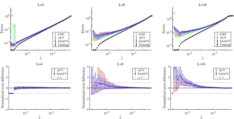
Fig. 1 shows the plots of the prediction and training errors against ˜λforL= 4,8,16 at N = 200 and σ_ξ2 = 0.01. This demonstrates that both approximations provide consistent results with the literal LOO CV, except at small ˜λs. This inconsistency at small ˜λs is considered to be due to a numerical instability occurring in the literal CV. Actually, for small ˜

λs, we have observed that certain small changes in the data induce large differences in the literal CV result. This example demonstrates that our approximations provide robust curves even in such situations. Note that asLgrows the number of estimated parameters{wa}La=1 increases while the data size M =αN = 400 is fixed, meaning that the problem becomes more and more underdetermined with the growth ofL. Hence, Fig. 1 demonstrates that the developed approximations work irrespectively of how much the problem is underdetermined. Fig. 2 exhibits the σ2_ξ-dependence of the errors and the approximation results forL= 8 and N = 200. For the very weak noise case (σ2

ξ = 0.001, left), the difference between the

predictive and training errors is negligible and hence all four curves are not discriminable. For the moderate (σ_ξ2= 0.1, middle) and large (σ2_ξ = 1, right) noise cases, the training curve is very different from the predictive ones. The approximation curves are again consistent with the literal LOO one.

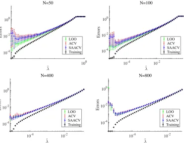
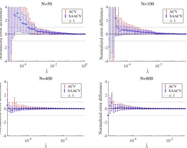
Fig. 3 demonstrates how the approximation accuracy changes as the system size N grows. For small sizes N = 50,100, a discriminable difference exists between the results of the approximations and the literal LOO CV, as well as the difference between the results of the two approximations. This is expected, because our derivation relies on the largeness of N and M. For large systems N = 400,800, the difference among the two approximations and the literal CV is much smaller. Considering this example in conjunction with the middle panel of Fig. 1, we can recognize that our approximate formula becomes fairly precise for N ≥200 in this parameter set. The normalized error difference corresponding to Fig. 3 is shown in Fig. 4. We can observe that the difference tends to be smaller as the system size increases, which is expected because the perturbation employed in our approximate formula is justified in the largeN, M limit.

Finally, let us consider the actual computational time to evaluate{wˆa}aand the

(14)

10-4 10-2 10-4

10-2 100

Errors

L=4

LOO ACV SAACV Training

10-4 10-2

10-4

10-2

100

Errors

L=8

10-4 10-2

10-4

10-2

100

Errors

L=16

10-4 10-2

-4 -2 0 2 4

Normalized error difference

L=4

ACV SAACV

1

10-4 10-2

-4 -2 0 2 4

L=8

ACV SAACV

1

10-4 10-2 -4

-2 0 2 4

L=16

ACV SAACV

1

(15)

10-4 10-3 10-2 10-4

10-3 10-2 10-1

Errors

2

=0.001

10-4 10-3 10-2 10-2

100

Errors

2

=0.1

10-4 10-3 10-2 10-2

100

Errors

2 =1

10-4 10-3 10-2 -4

-2 0 2 4

2 =0.001

ACV SAACV

1

10-4 10-3 10-2 -4

-2 0 2 4

2 =0.1

ACV SAACV

1

10-4 10-3 10-2 -4

-2 0 2 4

2

=1

ACV SAACV

1

(16)

100

10-4

10-2

100

Errors

N=50

10-4 10-2

10-4 10-2 100

Errors

N=100

10-4 10-2

10-4 10-2 100

Errors

N=400

10-4 10-2

10-4 10-2 100

Errors

N=800

(17)

10-4 10-2 100 -4

-2 0 2 4

N=50

ACV SAACV

1

10-4 10-2 -4

-2 0 2 4

N=100

ACV SAACV

1

10-4 10-2

-4 -2 0 2 4

N=400

ACV SAACV

1

10-4 10-2

-4 -2 0 2 4

N=800

ACV SAACV

1

(18)

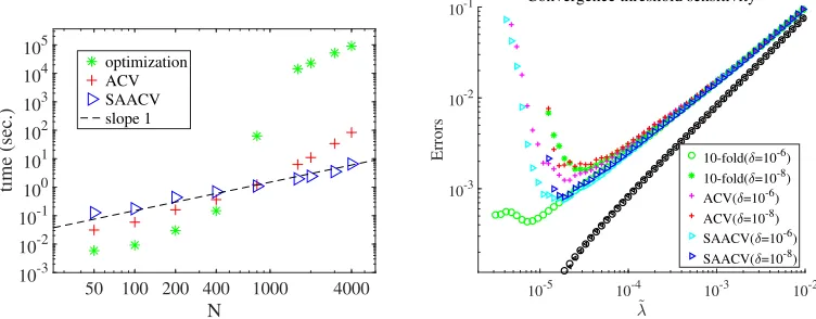
the plot of the actual computational time against the system size. Here, the number of examined points of ˜λto obtain a solution path is different from size to size, and hence the plotted time is given as the whole computational time to obtain the solution path divided by the number of ˜λs points. The left panel of Fig. 5 clearly displays the advantage and

50 100 200 400 1000 4000

N

10-3 10-2 10-1 100 101 102 103 104 105

time (sec.)

optimization ACV SAACV slope 1

10-5 10-4 10-3 10-2

10-3 10-2 10-1

Errors

Convergence threshold sensitivity

10-fold( =10-6) 10-fold( =10-8) ACV( =10-6) ACV( =10-8) SAACV( =10-6) SAACV( =10-8)

Figure 5: (Left) Actual computational time spent to find the solution of eq. (4) and that for ACV and SAACV, plotted against the feature dimensionality N in a double logarithmic scale. Note that the computational time for thek-fold CV is about k times larger than that for finding the solution of eq. (4), represented by the green asterisks. Parameters are fixed at L = 8, σ2

ξ = 0.01, α = 2 and ρ0 = 0.5.

Here,η= 1. (Right) The errors are obtained for the two convergence thresholds δ= 10−6 andδ= 10−8. Error bars are omitted for visibility. For the tighter case δ= 10−8, the minimum value of ˜λin the examined range is larger than that of the caseδ= 10−6, though the systematic difference with the results of the literal LOO CV is already clear. The training errors of these two differentδ, represented by black circles and left-pointing triangles, are completely overlapping. The system parameters areN = 400, L= 8,σ_ξ2 = 0.01,α= 2 and ρ0 = 0.5. Here,η= 1.

disadvantage of the developed approximations. For small sizes, the computational time for optimization to obtain{wˆa}ais shorter than the time to compute the approximate LOOEs,

(19)

indicator to verify the tightness of the convergence threshold. This is beneficial, especially when treating large models, for which the convergence check is a common annoying task.

3.2. On real-world dataset

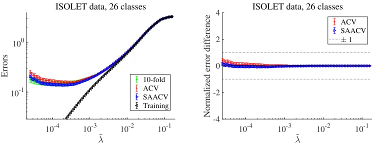
Next, we test the approximate formula on a real-world dataset. As shown above, our approximations become more precise if the model dimensionality and data size are large. Hence, we chose the ISOLET dataset which is a relatively large problem among classifica-tion tasks collected in the UCI machine learning repository (Lichman, 2013). The feature dimensionality, the data size, and the class number are N = 617, M = 6238, and L= 26, respectively. Here we apply the 10-fold CV, instead of the LOO CV because of the compu-tational reason, and our approximations to this dataset. The result is given in Fig. 6. The

10-4 10-3 10-2 10-1

10-1 100

Errors

ISOLET data, 26 classes

10-fold ACV SAACV Training

10-4 10-3 10-2 10-1

-4 -2 0 2 4

ISOLET data, 26 classes

ACV SAACV

1

Figure 6: Approximate CV performance on the ISOLET data of L = 26 classes. The errors are shown in the left panel and the normalized error differences between the approximations and the 10-fold CV are in the right panel. At the estimated minimums of the prediction error, the accuracy rate for correctly classifying the test data is about 0.86 while the probability of recovering the training data is about 0.98, commonly among the literal CV and the two approximations. At the minimum value of ˜λ, the leftmost point in the figure, the accuracy rates are different among the three different methods, and are 0.83,0.78, and 0.81 for the literal CV, ACV and SAACV, respectively. Here,η= 1.

(20)

3.3. When does SAACV fail?

Two major factors neglected in SAACV are the correlations among feature components and the heterogeneity among feature vectors. If these factors are strong, the approximation accuracy of SAACV is expected to be degraded. In this section, we examine this point.

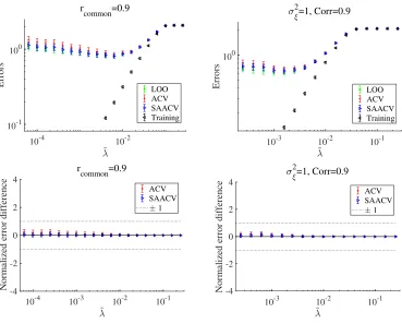
First, to test the impact of correlations in feature components, we add further constraints to the simulated data treated in sec. 3.1 and examine the approximation performance on the situation. Two cases are treated: the first is the case where the true feature vectors {w0a} have common components among all the classes. The result of this case is shown

in the left panels in Fig. 7. Here, the fraction of the common components to the non-zero components isrcommon= 0.9 and thus the overlap between feature vectors of different classes is rather large. The other is the case where the noise vector has strong correlations among the components. The result of this case is presented in the right panels in Fig. 7, in which the noise strength isσ_ξ2= 1 and the correlation coefficient of any pair of noise components is Corr(ξi, ξj) = 0.9; hence the noise and the correlation are rather large. For both the cases,

the performance of the approximate formula is fairly good, implying that SAACV is likely to perform well even when components of the feature vectors are correlated. Similar findings were actually obtained in the case of linear models (Obuchi and Kabashima, 2016). This is a preferable observation because it implies that the applicable limit of SAACV can be extended to a wider class of feature vectors than that is assumed in our present derivation in which the weakness of the correlations is assumed, as seen in sec. A. These also imply that there possibly exists another approximation formula taking into account the correlations but being similar to SAACV. A promising framework to derive such a formula might be the adaptive TAP method (Opper and Winther, 2001a,b, 2005). The adaptive TAP method itself requires a larger computational cost than that of SAACV but it is possible to reduce the computational cost up to the linear scaling with respect to N and M by employing an additional simplifying approximation (Kabashima and Vehkaper¨a, 2014; C¸ akmak and Opper, 2018). This is, however, rather technical and we leave it as a future work.

Second, to examine the effect of the heterogeneity among feature vectors, we introduce an amplifying factor Ω to control the norm of feature vectors. In particular, we multi-ply the factor Ω to the feature vectors of some chosen classes, as xµ → Ωxµ. Here, we

use the simulated data identical to that for the center panels in Fig. 3 of the parameters (N, L, α, ρ0, σξ2, η) = (200,8,2,0.5,0.1,1), except that the amplifying factor Ω = 100 is

(21)

10-4 10-2

10-1

100

Errors

r

common=0.9

10-3 10-2 10-1

100

Errors

2

=1, Corr=0.9

10-4 10-3 10-2 10-1

-4 -2 0 2 4

r

common=0.9

ACV SAACV

1

10-3 10-2 10-1 -4

-2 0 2 4

2

=1, Corr=0.9

ACV SAACV

1

Figure 7: (Upper) Log-log plots of the errors against ˜λ for correlated feature vectors. The left panel is for the case with common components in true feature vectors while the right one is of the correlated noise case. Parameters (N, L, α, ρ0, η) = (200,8,2,0.5,1) are common in both the cases, while the noise strengths and convergence thresholds are different: (σ2

ξ, δ) = (0.1,10−8) (left) and (σξ2, δ) =

(22)

10-3 10-2 10-1 0.5

1 1.5 2

Errors

=100

10-3 10-2 10-1

-4 -2 0 2 4

=100

ACV SAACV

1

Figure 8: (Left) Log-log plots of the errors against ˜λwith strong heterogeneity in feature vectors. The same dataset as that of the center panels in Fig. 3 is used but the feature vectors for the classesyµ = 5,6,7,8 are amplified as xµ → Ωxµ by the

factor Ω = 100. The ACV result is consistent with the LOO CV one while that of SAACV is not. (Right) The normalized error difference corresponding to the left panel.

can naturally emerge in some applications: for example if we consider problems in medical statistics, a number of biological markers can give distinguishably large values for affected patients compared to unaffected ones, yielding larger values in norm for feature vectors of affected patients. This consideration suspects the efficiency of SAACV. We, however, stress that this kind of heterogeneity attributed to the belonging class can be absorbed by rescaling the weights as{wa}a→ {Ω−1a wa}a, where Ωais chosen to homogenize the feature

vector norm in different classes as ||x_y_µΩa||2 ≈const. For the `1 regularization case, this resultantly leads to the regularization coefficients which take different values adaptively to the belonging class as

λX

a

||wa||1 →

X

a

λΩa||wa||1 =

X

a

λa||wa||1. (50)

For this problem with adaptive regularization coefficients, our approximation formula can be applied in the completely same manner, which can be convinced by seeing Algs. 1,2 where the value of the regularization coefficient is not required as the argument. The`2-norm can also be handled, though the codes should be extended to take into account the groupwise coefficients as arguments. We argue that this rescaling is a natural prescription to treat strong heterogeneity among different classes, and once employing this prescription the weak point of SAACV is naturally cured.

As a noteworthy remark, we point out that the basic idea of SAACV is closely related to Wahba’s generalized cross-validation (GCV) for linear regression (Golub et al., 1979). In GCV, the heterogeneity in coefficient corresponding toCµ\µin SAACV is also neglected, and

(23)

10-4 10-3 10-2 10-3

10-2

Errors

mnist (2 class), N=350, =1

10-4 10-3 10-2

10-3 10-2

Errors

10-4 10-3 10-2

-4 -2 0 2 4

ACV SAACV

1

10-4 10-3 10-2

-4 -2 0 2 4

ACV SAACV

1

(24)

reducing the computational cost is again needed because the data size and the model di-mensionality are increasing rapidly in recent years.

4. Conclusion

In this paper, we have developed an approximate formula for the CV estimator of the predictive likelihood of the multinomial logistic regression regularized by the `1-norm. An extension to the elastic net regularization has been also stated. We have demonstrated their advantages and disadvantages in numerical experiments using simulated and real-world datasets. Two versions of the approximation have been defined based on the developed formula. The first version, abbreviated as ACV, has a better performance, in terms of computational time, for middle size problems. It will eventually become worse than the literal k-fold CV with moderate ks as the problem size grows, because its computational time is scaled as a third-order polynomial of the feature dimensionality and data size, N and M, though such a tendency has not been observed in the investigated range of N. We have also defined the second version based on ACV, the computational time of which is just scaled linearly with respect toN andM. This second approximation is called SAACV, and it has been demonstrated that SAACV is slow for small size problems but has a great advantage for large size problems. Hence, we suggest leveraging the literal CV for small, ACV for middle, and SAACV for large size problems.

Our derivation is based on the perturbation which assumes that there is a small difference between the full and leave-one-out solutions. This assumption will not be satisfied for some specific cases. Even with this restriction, we expect the range of application of our formula is wide enough and we would like to encourage readers to leverage it in their own work. We have implemented MATLAB and python codes and they are available in (Obuchi, 2017; Takahashi and Obuchi, 2017).

The perturbative approach employed here is fairly general and can be applied to a wide class of generalized linear models with convex regularizations. The development of practical formulas for these cases will be of great assistance, given that we are living in the Big Data era.

Acknowledgments

This work was supported by JSPS KAKENHI Nos. 18K11463 (TO), 25120013 and 17H00764 (YK). TO is also supported by a Grant for Basic Science Research Projects from the Sum-itomo Foundation. The authors are grateful to Takashi Takahashi for implementation of the approximation formula in python.

Appendix A. The SA approximation

(25)

defining the so-called Boltzmann distribution:

P{w_a}L_a₌₁ D

M_{, λ}₌ 1

Z(DM_{, λ}₎e

−βH

{wa}La=1

D

M_,λ

= e −βP

a

λ1||wa||1+λ₂2||wa||22

Z(DM_{, λ}₎

M

Y

µ=1

φβ(yµ|{uµa}a). (51)

In the β → ∞ limit, this distribution converges to a point-wise measure of the solution of eq. (4) and hence, it is useful for analyzing eq. (51). We note that the BP is usually applied to graphical models having sparse tree-like structures, but is also applicable to ones with densely connected structures. In such applications, the BP can be regarded as a systematic implementation of the Thouless-Anderson-Palmer (TAP) approach (Thouless et al., 1977) in statistical physics, which can yield a set of self-consistent equations of the first and second moments of variables in statistical models when the models are of densely connected types. This approach has been applied to many different models in machine learning, which continuously yields evidences of its effectiveness (Opper and Winther, 1996, 1997, 2000a,b). When applied to densely connected models, certain correlations between variables have to be neglected to make the computation tractable; for that reason this approach, or the associated algorithm derived from it, is recently called approximate mes-sage passing (AMP) (Kabashima, 2003; Donoho et al., 2009). Basically, the AMP assumes that “interactions” between the variables are weak: in the present problem this implies (1/M)PM

µ=1xµixµj−

(1/M)PM

µ=1xµi (1/M)

PM

µ=1xµj

≈0 (i 6= j). This treatment can be justified if each feature vector xµ is i.i.d.. Rigorous proofs of this fact are available

for linear models and their some variants (Bayati and Montanari, 2011; Barbier et al., 2017). We implicitly assume this in the following derivation.

In this appendix, we introduce a new vector representation summarizing class variables: wi = (wai)a. Note that this is different from the notation used in the main body of this

paper, wa= (wai)i in which the feature components are summarized.

By regarding wi as a single variable node, the BP decomposes eq. (51) into two types

of messages as follows:

˜

Mµ→i(wi) =

Z Y

j(6=i)

dwj φβ(uµ)

Y

j(6=i)

Mj→µ(wj), (52)

Mi→µ(wi) =e

−β

λ1||wi||1+λ₂2||wi||22

Y

ν(6=µ) ˜

Mν→i(wi), (53)

whereuµ= (uµa)a. A crucial observation to assess eqs. (52,53) is that the argument of the

potential functionφ(uµ) has a sum of an extensive number of random variables; the central

limit theorem thus justifies treating it as a Gaussian variable with the appropriate mean and variance. Hence, according to eq. (52) wherewi is special, we can divide the extensive

sum as follows:

uµa =

X

j

xµjwaj =xµiwai+

X

j(6=i)

xµjwaj ≈xµiwai+

X

j(6=i)

(26)

where the second term on the right-hand side represents the mean of P

j(6=i)xµjwaj, the

symbolh·i\µdenotes the average over the Boltzmann distribution without theµth potential function, and tµ = (tµa)a denotes the zero-mean Gaussian variables whose covariance is

set to be that of

P

j(6=i)xµjwaj

a. This expression allows us to replace the integration

R Q

j(6=i)dwj by that overtµ in eq. (52). This significantly simplifies the computation and

yields:

˜

Mµ→i(wi)≈

Z

dteβ

−1

2t

>₍_C\µ

µ )−1t−qµ(wi,t)

≡

Z

dteβfµ(wi,t) ₍₅₅₎

where qµ(wi,t) is the negative log-likelihood whose argument uµa is approximated by eq.

(54) andCµ\µis the rescaled covariance of Pj(6=i)xµjwaj defined as

χ\₍_aiµ₎₍_bj₎≡β

hwaiwbji\µ− hwaii\µhwbji\µ

,

C_µ\µ

ab

≡X

i,j

xµixµjχ

\µ

(ai)(bj). (56)

In the second equation we added the contribution from ifor simplicity. It does not affect the following result because theith term contribution is small enough. Let us focus on the limit β → ∞. This limit allows us to use the saddle-point method, or Laplace’s method, with respect totµ. The associated saddle-point equation is:

ˆ

tµ=−C_µ\µbµ(wi,tˆµ), (57)

where bµ(wi,tˆµ) is the gradient of qµ defined at eq. (14) but the argument uµa is

approx-imated by eq. (54). Now, let us expand the exponent fµ(wi,t) in eq. (55) with respect to

the dynamical variables wi up to the second order. Putting za=P_ixµiwai, we can define

the derivatives as:

∂tˆµ

∂z_a =−(IL+C \µ µ Fµ)

−1

C_µ\µF∗µa, (58)

∂ fµ(wi,tˆµ)

∂z_a =−b

µ

a(wi,ˆtµ), (59)

∂2fµ(wi,tˆµ)

∂za∂zb

=−F_abµ −

∂tˆµ ∂z_a

>

F_∗µ_b =−

IL+FµCµ\µ

−1

Fµ

ab

. (60)

Hence,

˜

Mµ→i(wi)∝e

β(hµ_i)>wi−1₂w>i Γ µ iwi

(61)

where

hµ_i =−xµibµ,

Γµ_i =x2_µi(IL+FµCµ\µ)−1Fµ. (62)

(27)

Collecting all the messages except forµ, we can construct the LOO marginal distribution of wi as:

P\µ(wi)∝e

−β

λ1||wi||1+λ₂2||wi||22

Y

ν(6=µ) ˜

Mν→i(wi)

∝eβ(( P

ν(6=µ)h µ i)

>_w

i−12w

> i (λ2IL+

P

ν(6=µ)Γ µ

i)wi−λ1||wi||1)_. ₍₆₃₎

Now, we can close the equation for the rescaled variance

χ\_iµ

ab ≡ χ

\µ

(ai),(bi), because we can compute the variance ofwi from eq. (63). By considering the scaling, we can recognize

that the variances vanish in the speed ofO(β−2) if one of the two components or both are inactive. The active-active components of the variance are scaled byO(β−1) and remain in the rescaled variance. Focusing on the limit β→ ∞, we thus obtain:

χ\_iµ ˆ

AiAˆi

=



λ2I|_Aˆ_i|+



 X

ν(6=µ) Γν_i





ˆ

AiAˆi





−1

≈ λ2I|_Aˆ_i|+

X

ν

Γν_i

!

ˆ

AiAˆi

!−1

. (64)

At the last step, theµth term is added since its contribution is expected to be small enough in the summation. This manifests that the µ-dependence of χ\µ can be neglected and we rewrite it as χ\µ = χ hereafter. By considering the meaning of the Hessian, it is easy to understand thatG\µ _{is identified with}_λ

2IL+Pν(6=µ)Γνi

. This yields eq. (40). By assuming the vanishing correlation between wi and wj fori6=j, we can write

χ₍_ai₎₍_bj₎ ≈δij

(χi)_ab (a, b∈Aˆi)

0 (otherwise) . (65)

These leads to:

C_µ\µ

ab=

X

ij

xµixµjχ\₍_aiµ₎₍_bj₎≈

X

i

x2_µi(χi)_ab≈σ2x

X

i

(χi)_ab≡(CSA)_ab (66)

Theµ-dependence throughx2_µiis neglected at the last step, because the sumP

iwould mask

such a weak µ-dependence as long as strong heterogeneity in {xµi}µ is absent. Similarly,

we may write the sum inside the parentheses of the righthand side of eq. (64) as:

X

ν

Γν_i ≈σ_x2X

ν

(IL+FνCSA)−1Fν. (67)

Inserting eqs. (65-67) into eq. (64), we obtain eq. (41).

Careful readers may be concerned about the neglected µ-dependence ofχ\µ, as well as that of G\µ. If this can be neglected, may we replaceG\µ with G from the beginning at eq. (21)? The answer is of course no. The reason is that the difference between G\µ andG is not negligible if they are “projected” onto Xµ as in eq. (21). If they are projected onto other directions perpendicular to Xµ, the difference is actually tiny and can be neglected, but for computing the factorCµ\µwe need to take into account this difference appropriately.

(28)

factor C is computed based on neglecting the difference between G and G\µ. As a result we cannot discriminate the two factors Cµ and C

\µ

µ . This consideration implies that our

SA estimation ofC,CSA, should be applied toCµ\µ in eq. (21) and should NOT be applied

to Cµ in eq. (24), because the latter formula formally takes into account the difference in

advance.

References

Tomohiro Ando and Ruey Tsay. Predictive likelihood for bayesian model selection and averaging. International Journal of Forecasting, 26(4):744–763, 2010.

Jean Barbier, Nicolas Macris, Mohamad Dia, and Florent Krzakala. Mutual information and optimality of approximate message-passing in random linear estimation. arXiv preprint arXiv:1701.05823, 2017.

Mohsen Bayati and Andrea Montanari. The dynamics of message passing on dense graphs, with applications to compressed sensing. IEEE Transactions on Information Theory, 57 (2):764–785, 2011.

Jan F Bjornstad. Predictive likelihood: a review. Statistical Science, pages 242–254, 1990.

Burak C¸ akmak and Manfred Opper. Expectation propagation for approximate inference: Free probability framework. CoRR, abs/1801.05411, 2018. URL http://arxiv.org/ abs/1801.05411.

David L Donoho, Arian Maleki, and Andrea Montanari. Message-passing algorithms for compressed sensing. Proceedings of the National Academy of Sciences, 106(45):18914– 18919, 2009.

Jerome Friedman, Trevor Hastie, and Rob Tibshirani. Regularization paths for generalized linear models via coordinate descent. Journal of statistical software, 33(1):1, 2010.

Gene H Golub, Michael Heath, and Grace Wahba. Generalized cross-validation as a method for choosing a good ridge parameter. Technometrics, 21(2):215–223, 1979.

Yoshiyuki Kabashima. A CDMA multiuser detection algorithm on the basis of belief prop-agation. Journal of Physics A: Mathematical and General, 36(43):11111, 2003.

Yoshiyuki Kabashima and Mikko Vehkaper¨a. Signal recovery using expectation consistent approximation for linear observations. In Information Theory (ISIT), 2014 IEEE Inter-national Symposium on, pages 226–230. IEEE, 2014.

Balaji Krishnapuram, Lawrence Carin, Mario AT Figueiredo, and Alexander J Hartemink. Sparse multinomial logistic regression: Fast algorithms and generalization bounds. IEEE transactions on pattern analysis and machine intelligence, 27(6):957–968, 2005.

(29)

M. Lichman. UCI machine learning repository, 2013. URLhttp://archive.ics.uci.edu/ ml.

Tomoyuki Obuchi. Matlab package of ACV on MLR. https://github.com/T-Obuchi/ AcceleratedCVonMLR_matlab, 2017.

Tomoyuki Obuchi and Yoshiyuki Kabashima. Cross validation in lasso and its acceleration.

Journal of Statistical Mechanics: Theory and Experiment, 2016(5):53304–53339, 2016.

Tomoyuki Obuchi, Shiro Ikeda, Kazunori Akiyama, and Yoshiyuki Kabashima. Accelerating cross-validation with total variation and its application to super-resolution imaging. PloS one, 12(12):e0188012, 2017.

Manfred Opper and Ole Winther. Mean field approach to bayes learning in feed-forward neural networks. Physical review letters, 76(11):1964, 1996.

Manfred Opper and Ole Winther. A mean field algorithm for bayes learning in large feed-forward neural networks. In Advances in Neural Information Processing Systems, pages 225–231, 1997.

Manfred Opper and Ole Winther. Gaussian processes and SVM: Mean field results and leave-one-out, pages 43–65. MIT, 10 2000a. ISBN 0262194481. Massachusetts Institute of Technology Press (MIT Press) Available on Google Books.

Manfred Opper and Ole Winther. Gaussian processes for classification: Mean-field algo-rithms. Neural computation, 12(11):2655–2684, 2000b.

Manfred Opper and Ole Winther. Adaptive and self-averaging thouless-anderson-palmer mean-field theory for probabilistic modeling. Physical Review E, 64(5):056131, 2001a.

Manfred Opper and Ole Winther. Tractable approximations for probabilistic models: The adaptive thouless-anderson-palmer mean field approach. Physical Review Letters, 86(17): 3695, 2001b.

Manfred Opper and Ole Winther. Expectation consistent approximate inference. Journal of Machine Learning Research, 6(Dec):2177–2204, 2005.

Kamiar Rahnama Rad and Arian Maleki. A scalable estimate of the extra-sample prediction error via approximate leave-one-out. arXiv preprint arXiv:1801.10243, 2018.

Mark Schmidt. Graphical model structure learning with l1-regularization. University of British Columbia, 2010.

Takashi Takahashi and Tomoyuki Obuchi. Python package of ACV on MLR. https: //github.com/T-Obuchi/AcceleratedCVonMLR_python, 2017.

(30)

Hastie Trevor, Tibshirani Robert, and Friedman Jerome.The Elements of Statistical Learn-ing; Data Mining, Inference, and Prediction. Springer-Verlag New York, 2009. doi: 10.1007/978-0-387-84858-7.

Vladimir Vapnik and Olivier Chapelle. Bounds on error expectation for support vector machines. Neural computation, 12(9):2013–2036, 2000.

Shuaiwen Wang, Wenda Zhou, Haihao Lu, Arian Maleki, and Vahab Mirrokni. Ap-proximate leave-one-out for fast parameter tuning in high dimensions. arXiv preprint arXiv:1807.02694, 2018.