Smooth neighborhood recommender systems

Smooth neighborhood recommender systems

Ben Dai bendai2-c@my.cityu.edu.hk

Junhui Wang j.h.wang@cityu.edu.hk

School of Data Science City University of Hong Kong Kowloon Tong, 999077, Hong Kong

Xiaotong Shen xshen@umn.edu

School of Statistics University of Minnesota Minneapolis, MN 55455, USA

Annie Qu anniequ@illinois.edu

Department of Statistics

University of Illinois at Urbana Champaign Champaign, IL 61820, USA

Editor:Gert Lanckriet

Abstract

Recommender systems predict users’ preferences over a large number of items by pooling similar information from other users and/or items in the presence of sparse observations. One major challenge is how to utilize user-item specific covariates and networks describing user-item interactions in a high-dimensional situation, for accurate personalized prediction. In this article, we propose a smooth neighborhood recommender in the framework of the latent factor models. A similarity kernel is utilized to borrow neighborhood information from continuous covariates over a user-item specific network, such as a user’s social network, where the grouping information defined by discrete covariates is also integrated through the network. Consequently, user-item specific information is built into the recommender to battle the ‘cold-start” issue in the absence of observations in collaborative and content-based filtering. Moreover, we utilize a “divide-and-conquer” version of the alternating least squares algorithm to achieve scalable computation, and establish asymptotic results for the proposed method, demonstrating that it achieves superior prediction accuracy. Finally, we illustrate that the proposed method improves substantially over its competitors in simulated examples and real benchmark data–Last.fm music data.

Keywords: Blockwise coordinate decent, Cold-start, Kernel smoothing, Neighborhood, Personalized prediction, Singular value decomposition, Social networks.

1. Introduction

Recommender systems predict users’ preferences over a large number of items by pooling similar information from other users or items when observations are sparse, which are particularly useful in personalized prediction. It has become an essential part of e-commerce, with applications in movie rentals (MovieLens; Miller et al. 2003), restaurant guides (Entree;

Burke 2002), book recommendations (Amazon; Linden et al. 2003), and personalized e-news (Daily learner; Billsus and Pazzani 2000).

Two main streams emerge for training recommender systems: collaborative filtering, which predicts users’ behaviors based on similar users (Bell and Koren, 2007), and content-based filtering, which builds user and item profiles content-based on domain knowledge and rec-ommends items with similar profiles (Lang, 1995; Melville et al., 2002). Specifically, col-laborative filtering predicts unknown ratings by averaging over similar users’ ratings with weights; such as the latent factor approach (Feuerverger et al., 2012), latent Dirichlet alloca-tion (LDA; Blei et al. 2003), probabilistic latent semantic analysis (pLSA; Hofmann 2004), regularized singular value decomposition (regularized SVD; Paterek 2007), and restricted Boltzmann machines (RBM; Salakhutdinov et al. 2007). Among them, the regularized SVD approach has become popular due to its high predictive performance and scalability in real applications. In addition, Koren (2008) further generalizes SVD to model users’ implicit feedbacks, and Forbes and Zhu (2011) incorporates content information in the regularized SVD approach through a regression-type of constraint. For content-based filtering, keywords analysis extracts features from items previously rated by a user to develop a profile of the user’s interests, and recommendation is made by comparing the user profile and potential items (Lang, 1995). The naive Bayes (Billsus and Pazzani, 2000), decision tree (Pazzani et al., 1996) and kNN (Middleton et al., 2004) formulate this type of recommendation as a classification problem, where each item can be labeled by users as “like” or “dislike”. Hybrid recommender systems (Burke, 2002) utilize geo-social correlations to accommodate new users and items through location-based recommendation systems; Bi et al. (2017) pro-poses a group-specific latent factor model by utilizing missingness-related characteristics to accommodate new users or items without any observed ratings.

usu-ally does not follow a parametric form in terms of covariates, which is commonly assumed in the literature due to the lack of sufficient observations for each user and item. How to employ a nonparametric approach to model the covariate-assisted recommender system in a high-dimensional setting continues to be an open question. Third, missing completely at random (MCAR) is often assumed by existing methods, leading to inaccurate prediction as the MCAR assumption is typically unrealistic for recommender systems. For example, users tend not to rate items that are of little interest to them, as illustrated in Figure 4. Fourth, most methods fail to recommend for new users or items without any observed rat-ings, which is referred as the “cold-start” problem. Thus, utilizing the covariate information to fully and efficiently solve the “cold-start” problem is attractive in devising recommender systems.

In this paper, we propose a novel approach based on the idea of a similarity-based neighborhood system pooling similar user-item pairs to improve prediction performance. Specifically, for each user-item pair, the proposed approach incorporates similar observed pairs through kernel weighting based on covariates as well as a user-item specific network. The weight function quantifies a smooth rating mechanism in terms of the closeness of continuous covariates within a neighborhood of the connected user-item pairs in the network. One novelty of the proposed approach is that it builds discrete covariates into a user-item specific network with the same discrete covariate values corresponding to connectivity. This enables us to handle high-dimensional covariates while not being burdened by the “curse of dimensionality.” Unlike existing methods (Zhu et al., 2016; Bi et al., 2017), our approach is nonparametric, yet it goes beyond the traditional nonparametric framework which focuses primarily on continuous covariates. This provides a flexible framework to handle continuous covariates, discrete covariates and networks all together without specifying a functional relation. Moreover, the proposed approach also tackles the “cold-start” issue as it utilizes observed pairs in the neighborhood of any new user-item pairs in prediction.

The proposed approach takes full advantage of the smoothing pattern of the rating mech-anism over covariates, while integrating user-item dependencies through user-item specific networks into a recommender system nonparametrically. This leads to a higher predic-tion accuracy for a recommender, as demonstrated in the numerical examples in Secpredic-tion 5. Significantly, our approach outperforms the state-of-the-art prediction performance for the Last.fm music benchmark dataset by nearly 20%. Additionally, we perform an error analysis, showing that the error rate of the proposed method is governed by the degree of smoothness of a neighborhood system with respect to continuous covariates, given that the grouping information is precisely defined by discrete covariates and networks. Most critically, as suggested by Theorem 1, the method performs well even in a high-dimensional situation in which the overall size of observed ratings is of the same magnitude as the number of unknown parameters.

2. Regularized latent factors

In this section, we provide the notations in recommender systems, and the framework of a regularized latent factor model. Consider a recommender system of n users’ preference scores on m items, where rui denotes the preference score of user u on item i. Suppose a user-item specific covariate vector xui ∈ X ⊂ Rd is observed (e.g., a user’s demographics

and an item’s content information). One key challenge for training a recommender system is that the preference matrixR= (rui)∈Rn×m is only partially observed with a high missing

percentage. Denote the index set of observed preference scores as Ω, then |Ω| nm. A recommender system can be formulated in the framework of a latent factor model:

rui=θui+ui=pTuqi+εui, 1≤u≤n,1≤i≤m, (1)

where θui = E(rui) is the expected preference score of a user-item pair (u, i), and εui is independent fromxui with mean zero and finite variance. The latent factor model assumes that θui can be represented by user and item latent factors: θui = pTuqi, where pu and

qi are K-dimensional latent vectors representing user u’s preference and item i’s profile, respectively, and K is the number of latent factors for both users and items, which is also the rank in the latent factor model (Mukherjee et al., 2015).

To estimate these personalized parameters, a regularized SVD method (Paterek, 2007; Zhu et al., 2016) estimatesP = (p1,· · ·,pn)T and Q= (q1,· · · ,qm)T by

min P,Q

1 |Ω|

X

(u,i)∈Ω

(rui−pTuqi)2+λ

n X

u=1

J(pu) + m X

i=1

J(qi) , (2)

where λis a nonnegative tuning parameter, and J(·) can be any penalty function such as the Lq-penalty with q = 0,1,2 (Zhu et al., 2016) or the alignment penalty (Nguyen and Zhu, 2013). Note thatruiin (2) is often replaced by the residualrui−µ−xTuiβ, where (µ,β) is a vector of regression coefficients to be minimized in (2). Alternatively, pu =su−xTuα and qi = ti −xTi β, where (su,ti) are latent factors, and (α,β) are regression coefficients to incorporate the covariate effects (Agarwal et al., 2011).

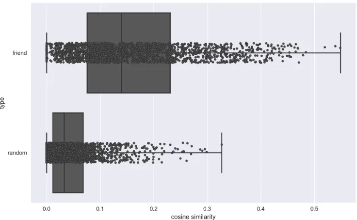
There are a number of major challenges for the regularized SVD model in (2). First, a user-item specific network is often available to capture user-item dependence but is ignored in (2). Here networks consists of information from existing users’ social network, or item network, or the network constructed from available discrete covariates of the user-item pair (u, i). It can provide additional information regarding the preference similarity between connected pairs. This is the case for the Last.fm data, where a user specific network impacts users’ preference on items, indicated by Figure 1. Second, a linear model in (2) may be inadequate to incorporate user and item covariates, especially when the linearity assumption is violated. Third, the objective function (2) assumes implicitly that missing occurs completely at random so that the first loss function in (2) can approximate the loss function for the complete data. When the missing is informative, missing characteristics such as the missing pattern for each user can be utilized for subgrouping (Bi et al., 2017). Fourth, the regularized SVD in (2) suffers from the “cold-start” problem for new users or items in the absence of observed ratings. For instance, if a useru or an itemiis completely missing from Ω, the corresponding pu orqi is estimated incorrectly as 0 due to the penalty

Figure 1: Comparison of the cosine similarity of logarithm of users’ listening counts vector between friends and randomly selected users in the Last.fm dataset.

3. Methods

This section introduces a smooth recommender system, which incorporates user and/or item specific covariates and the user-item specific network information to improve prediction accuracy. The proposed method utilizes informative observations for each user-item pair for personalized prediction and resolving the “cold-start” problem.

3.1. Proposed method

One key strategy of the proposed method is to pool information across user-item pairs to improve prediction accuracy through increasing effective sample size. In contrast to grouping approaches based on user-item-specific information (Bi et al., 2017; Masthoff, 2011), the proposed recommender system integrates similar observed pairs (u0, i0) ∈Ω for each (u, i) through a weight function, regardless of whether (u, i) is observed or not. This allows for nonlinear or nonparametric modeling of the relation between user-item preferences and latent factors, which is more flexible than the linear modeling in (2).

in the Last.fm dataset, rui is the listening count of a user-artist pair (u, i), and xui is the pattern of listening counts for useruand artisti. The available network information is given as S_uui0_i0 =S_uu0Si_i0, where S_uu0 represents a user’s friendship network, and S_ii0 is constructed from artists’ tag information with S_ii0 = 1 indicating artists i and i0 share the same tags, and S_ii0 = 0 otherwise.

Using local likelihood via smoothing weights (Tibshirani and Hastie, 1987; Fan and Gij-bels, 1996), we propose the following cost function for a smooth neighborhood recommender system:

L(P,Q) = 1 nm n X u=1 m X i=1 _X

(u0_,i0_)∈Ω

ωui,u0_i0(r_u0_i0−pT_uq_i)2

+λ1

n X

u=1

J(pu) +λ2

m X

i=1

J(qi), (3)

where J(·) is a general penalty, and λ1 and λ2 are two nonnegative tuning parameters. It

is also assumed thatP

(u0_,i0_)∈Ωω_ui,u0_i0 = 1. Lemma 1 below gives an equivalent form of (3). Lemma 1 The cost function L(P,Q) in (3) is equivalent to

1 nm n X u=1 m X i=1 _X

(u0_,i0_)∈Ω

ωui,u0_i0r_u0_i0 −pT_uq_i

2 +λ1

n X

u=1

J(pu) +λ2

m X

i=1

J(qi). (4)

The choice of ωui,u0_i0 is critical to properly measure the similarity between (u, i) and (u0, i0). We introduce a weight function to define the smooth neighborhood of (u, i):

ωui,u0_i0 =

Kh(xui,xu0_i0)Sui

u0_i0

P

(u0_,i0_)∈ΩKh(xui,xu0_i0)Sui

u0_i0

, (5)

where ωui,u0_i0 involves only observed pairs (u0, i0)’s with Sui

u0_i0 = 1. In (5), ifxui orS_uui0_i0 is absent,K_h(xui,xu0_i0) orSui

u0_i0 can be set as 1 correspondingly. The kernel function is set as

Kh(xui,xu0_i0) =K(h−1kx_ui−x_u0_i0k₂) measuring the closeness betweenx_uiandx_u0_i0, where the choice of the L2-norm reduces the dimension of the covariate space and other choices

of distance may be also considered. Here h > 0 is the window size and K(·) is a kernel whose degree of smoothness reflects prior knowledge about how the true preference varies in terms ofkxui−xu0_i0k₂. Note that this is different from standard kernel smoothing (Fan and Gijbels, 1996; Delaigle and Hall, 2010), in that the smooth neighborhood is constructed based on continuous and discrete covariates as well as user-item specific networks, whereas standard kernel smoothing focuses primarily on smoothing over continuous covariates.

The proposed framework has the following advantages. First, the user-item specific covariates and network structures are integrated in constructing the neighborhood for (u, i) pairs. Thus the effective sample size for (u, i) increases when pooling information from its neighborhood through P

(u0_,i0_)∈Ωω_ui,u0_i0r_u0_i0 in (4). Second, it solves the “cold-start” problem and yields more accurate estimators of p_u and q_i for allu’s and i’s by leveraging dependencies among users and items, expressed in terms of user-specific social networks and items’ tagging information. This is evident from (4), since even for an unobserved (u, i), P

pair (u, i). Third, the non-ignorable missing can be addressed through a covariate-adjusted neighborhood associated with missingness and users’ preferences. For instance, each user’s and item’s missing percentages and the percentiles of their observed ratings can be modeled nonparametrically as covariates in defining ωui,u0_i0.

3.2. Scalable computation

To solve large-scale optimization in (3), we employ a “divide-and-conquer” type of alter-nating least squares (ALS) algorithm, with a principle of solving many small penalized regression problems iteratively. This permits parallel and efficient computation. The ALS method has been extensively investigated in the literature (Carroll and Chang, 1970; Fried-man and Stuetzle, 1981), and the divide-and-conquer strategy is also employed in (Zhu et al., 2016) for the parallelization of (2).

The computational strategy of ALS is to break large-scale optimization into multiple small subproblems by alternatively fixing eitherpu orqi, where each subproblem is a simple penalized least squares regression and can be solved analytically with J(·) =k · k2

2. Note

that this strategy is applicable as long asJ(·) is separable forpu and qi. For illustration, consider J(·) =k · k2

2. At iterationk,Qb(k) is fixed and the latent factor

puis updated as ˆp(uk+1) = argminpu P

i

P

(u0_,i0_)∈Ωωui,u0_i0(r_u0_i0−pT_uqˆ(k)

i )2

+λ1kpuk22.

Sim-ilarly, with fixed Pb(k+1), q_i is updated as ˆq

(k+1)

i = argminqi P

u

P

(u0_,i0_)∈Ωωui,u0_i0(r_u0_i0− ( ˆp(uk+1))Tqi)2

+λ2kqik22.Then each subproblem is solved analytically,

ˆ

p(_uk+1) = X i

ˆ

q_i(k)( ˆq_i(k))T +λ1IK

−1 _X

i ¯ rΩ_uiqˆ_i(k)

, (6)

ˆ

q(_ik+1) = X u

ˆ

p_u(k+1)( ˆp_u(k+1))T +λ2IK

−1 _X

u ¯

r_uiΩpˆ(_uk+1)

, (7)

where ¯rΩ_ui=P

(u0_,i0_)∈Ωω_ui,u0_i0r_u0_i0 is a weighted rating for (u, i) over the neighborhood, and IK is a K ×K identity matrix. The iterative updating is continued until a termination criterion is reached. Once the solution{pˆu,qˆi}1≤u≤n;1≤i≤m is obtained, the final predicted preference is ˆrui= ˆpTuqˆi.

It follows from Chen et al. (2012) that the algorithm converges to a stationary point ( ¯P,Q¯) of L(P,Q) in (3), where ¯P = argmin_PL(P,Q¯), and ¯Q= argmin_QL( ¯P,Q). This is due to the nonconvex minimization in addition to having many missing observations. Moreover, each update of pu and qi in (6) and (7) can be computed in a parallel fashion. This can substantially speed up the computation, particularly whenK is small butm and nare large.

The overall computational complexity of the algorithm is no greater than O (nmK2+ (n+m)K3)IALS

4. Theory

This section presents theoretical properties to quantify the asymptotic behavior of the proposed recommender system. Particularly, we show the convergence rate in prediction error of the proposed system.

Let the true and estimated parameters be θ0

ui =p0u T

q0

i and ˆθui = ˆpTuqˆi, where ˆpu and ˆ

qi are estimated latent factors; u = 1,· · ·, n; i = 1,· · ·, m. Note that the representation is unique with respect toθui, although the decomposition ofpu and qi may not be unique. Let ˆθ = (ˆθui) ∈ Rn×m and θ0 = (θui0 ) ∈Rn×m, the prediction accuracy of ˆθ is defined by the root mean square error:

RMSE(θˆ,θ0) = 1 nm

n X

u=1

m X

i=1

ˆ θui−θui0

21/2

.

We require the following technical assumptions.

Assumption A. There exist constants c1 >0 and α > 0 such that for any (u, i) and

(u0, i0) , θ_ui0 −θ_u00_i0

≤ c₁

√

Kmax{kxui−xu0_i0kα₂, I(Sui

u0_i0 = 0)}, where the corresponding expression in the maximum operator is set as 0 ifxui orSuui0_i0 is absent.

Assumption A defines the smoothness of θ0

ui in terms of the continuous covariatexuiin the presence of connected user-item pairs in the network. As a special case, ifxui is absent, Assumption A degenerates toθ_ui0 =θ_u00_i0 for pairs with Sui_u0_i0 = 1. This assumption is mild when all covariates are available, and is relatively more restrictive when xui is absent as it pushes the model to be a parametric one with only a finite number of unknown θ’s. It is necessary to capture the smooth property of θ over the network structure, and similar assumptions are widely used in nonparametric regression (Vieu, 1991; Wassermann, 2006) and kernel density estimation (Stone, 1984; Marron and Padgett, 1987).

Assumption B. The continuous covariatex has a bounded supportX, and the error termεui has a sub-Gaussian distribution with varianceσ2.

Assumption B is a regularity condition for the underlying probability distribution, and widely used in literature (Ma and Huang, 2017; Lin et al., 2017). Further, assume that {xui,∆ui}1≤u≤n,1≤i≤m are independent and identically distributed, but the distribution of ∆uimay depend onxui. We denote the parameter spaceΓ(L) to be{θ:kθk∞≤L}, where

k · k∞ is the uniform norm, and L is chosen so that θ0 ∈ Γ(L). To accurately utilize the

network information, we setωui,u0_i0 = 0 ifSui

u0_i0 = 0. Theorem 1 establishes an upper bound for the estimation error of the proposed recommender system, where the convergence rate is determined by the size of the preference matrix nm, the number of parameters K, the size of the observed ratings |Ω|, the tuning parameters λ1 andλ2, and the window size h. Theorem 1 Suppose that Assumptions A and B are satisfied. For some constant c2 >0, let κ1 = maxu,iP(u0_,i0_)∈Ωω_ui,u0_i0kx_ui−x_u0_i0kα

2, andκ2= maxu,iP(u0_,i0_)∈Ωω_ui,u2 0_i0, then P RMSE( ˆθ,θ0)≥η≤exp−c2η

2 κ2

+ log(nm) ,

provided that η≥max√Kκ1,

√

κ2 log (nm) and λ1Pn_u=1J(p0u) +λ2Pm_i=1J(qi0)≤η2/4.

The convergence rate then becomes RMSE( ˆθ,θ0) =Op(max

√

Theorem 1 provides a general upper bound of RMSE( ˆθ,θ0), which may vary by the choice of weights ωui,u0_i0 and the two quantities κ₁ and κ₂. In the following, an explicit convergence rate is given forωui,u0_i0 defined in (5) under some additional assumptions.

Let ∆ui∈ {0,1}be a binary variable, with ∆ui= 1 indicating thatruiis observed and 0 otherwise. Assume that{xui,∆ui}1≤u≤n,1≤i≤m are independent and identically distributed, but the distribution of ∆ui may depend onxui.

Assumption C.For any (u, i) and (u0, i0),P(S_uui0_i0 = 1|∆u0_i0 = 1) is bounded away from zero, and the conditional densityf_Uui

u0i0|S ui

u0i0=1,∆u0i0=1 is continuous and bounded away from zero, whereU_uui0_i0 =kx_ui−x_u0_i0k₂.

Assumption C is necessary for tackling the “cold-start” problem, and similar assump-tions are also widely used in the local smoothing technique (Chen et al., 2014; Scott, 2015). It ensures that for any pair (u, i), the probability of ∆ui= 1 may depend on covariates xui and S_uui0_i0, and that the corresponding neighboring pairs are observed with positive proba-bility. In fact, it suffices to assume that P(S_uui0_i0 = 1|∆u0_i0 = 1) is bounded away from zero with certain order, and similar results can be obtained with more involved derivation.

Assumption D. There exists a constant c2 such that the nonnegative kernel K(·)

satisfies

max

nZ ∞

0

K2(u)du,

Z ∞

0

K(u)uαdu

o ≤c3.

Assumption D is a standard assumption for smoothing kernels. Notably, the choice of kernel should match up the smoothness at an order α of θ0. Alternatively, to effectively employ the smoothing pattern ofθ, the decay rate of the chosen kernel may be larger than α, to filter out more distant user-item pairs and preserve more reliable local neighborhood structure. For example, the Gaussian kernel has an exponential decay rate, and always satisfies the inequality conditions in Assumption D.

Corollary 1 Suppose that Assumptions A-D are satisfied. For ωui,u0_i0 defined in (5), then

the convergence rate of RMSE( ˆθ,θ0)becomes RMSE( ˆθ,θ0) =Op |Ω|− α 2α+1_K

1

2(2α+1)_log(nm).

Note that this convergence rate is intriguing compared with some existing results. Par-ticularly, when K =O(1), we have RMSE(θˆ,θ0) = OP |Ω|−

α

2α+1_{log(nm). For α > 1/2,}

since |Ω| ≤nm < (n+m)2_{, it leads to a tighter bound than O}

P

n+m

|Ω| log( √

nm

|Ω| )

1₂ and

OP

n+m

|Ω| log(m) log( |Ω|

n+m) 1₂

established in Bi et al. (2017) and Srebro et al. (2005),

re-spectively. In addition, Theorem 1 still guarantees the convergence of RMSE(θˆ,θ0), if K goes to infinity at a rate slower than |Ω|2α_(log(nm))−2(2α+1)_{. In practice, the size of Ω}

is often much less than nm, and only proportional to (n+m)K. For example, in the MovieLens 1M dataset with K = 10, nm = 0.2×108,|Ω| = 106, and (n+m)K = 106; and in the Last.fm dataset, nm = 0.3×108,|Ω| = 106 and (n+m)K = 0.2×106. In such cases with K = O(1), the theoretical results in Bi et al. (2017) and Srebro et al. (2005) fail to give a reasonable convergence rate. However, Theorem 1 still yields that RMSE(θˆ,θ0) = OP |Ω|−

α

2α+1_{log(nm). Interestingly, if the continuous covariates are} ab-sent, then Assumption A is satisfied withα =∞, and there is only a finite number of θ’s to be estimated for different discrete covariates. In such cases, Theorem 1 implies that the recommender system can be estimated with a rate η∼OP |Ω|−1/2log(nm)

5. Numerical results

This section examines the performance of the proposed method, denoted as sSVD, in sim-ulations and with a realLast.fm dataset. We compare sSVD to several strong competitors, including restricted Boltzmann machines (RBM; Salakhutdinov et al. 2007) or a continu-ous version of restricted Boltzmann machines (CRBM; Chen and Murray 2003); an iter-ative soft-threshold matrix completion method (SoftImpute; Hastie et al. 2015); the reg-ularized SVD (rSVD; Paterek 2007); the self-recovered side regression (SSR; Zhao et al. (2016)) and a group-specific SVD approach (gSVD; Bi et al. 2017). Note that the Python codes for RBM and CRBM are publicly available (https://github.com/yusugomori/ DeepLearning/tree/master/python), the code for SoftImpute is available in the Python package “fancyimpute”, the Matlab code for SSR is provided by Zhao et al. (2016), and the R code for gSVD is provided by Bi et al. (2017). Note that RBM and CRBM are essentially the same but differ in implementation only for discrete and continuous responses. Although RBM, SoftImpute and rSVD are not designed to incorporate covariates, we include them in comparison to illustrate the importance of utilizing covariates for personalized prediction.

For tuning parameter selection, we set the learning rate, the momentum rate and the number of hidden units for RBM and CRBM as 0.005, 0.9, and 100, respectively. For rSVD, gSVD and sSVD, we set the tuning parameter K to be the true one, and the optimal λ is determined by a grid search over {10(ν−31)/10;ν = 1,· · ·,61}. For the proposed sSVD, a Gaussian kernel is used with the window size h being the median distance among all user-item pairs. The predictive performance of all methods is measured by the root mean squared error (RMSE).

5.1. Simulated examples

This subsection investigates the “cold-start” problem and the utility of a user-item specific network on prediction performance. We generate the simulation setting as follows. The dimensions of a rating matrix {rui}1≤u≤n;1≤i≤m are n = 501 and m = 201. Let pu = (1 + 0.002u)1K+N(0K, ξIK) andqi = (1 + 0.0075i)1K+N(0K, ξIK) foru= 1,· · · , nand

i= 1,· · ·, m, where1Kand0K beingK-dimensional vectors of ones and zeros, respectively. Here we sample observed ratings at random, where π is the missing rate, and the total number of observed ratings is |Ω|= (1−π)nm. For each user-item pair (u, i)∈Ω, we letu and ibe uniformly sampled from 1,· · · , nand 1,· · · , m, respectively, and rui be generated from a truncated normal distribution on [1,5] with meanpT_uqi and standard deviation 0.5. Further, rui is rounded to the closest integer in {1,· · · ,5} to mimic discrete ratings in practice.

weight function is set as ωui,u0_i0 = Sui

u0_i0, which is constructed based on the adjacency of each user-item pairs. For gSVD, we use the ranking percentages of each user and item as covariates according to Bi et al. (2017), but the user-item specific network information is not incorporated.

Table 1: Averaged RMSEs of various methods and their estimated standard deviations in parentheses on the simulated examples over 50 simulations. Here RBM, SoftImput, rSVD, gSVD, sSVD denote: restricted Boltzmann machines (Salakhutdinov et al., 2007), SoftImput method (Hastie et al., 2015), regularized SVD method (Paterek, 2007), group-specific SVD method (Bi et al., 2017) and the proposed method, respectively. The best performer in each setting is bold-faced.

RBM SoftImpute SSR rSVD gSVD sSVD

Use of covariate No No Yes No Yes Yes

K= 3,π= 0.8

ρ= 0.0 0.842(0.001) 1.082(.003) 2.471(.002) 0.323(.000) 0.302(.000) 0.364(.001)

ρ= 0.1 0.911(0.003) 2.100(.007) 2.570(.004) 1.112(.009) 0.472(.003) 0.371(.001) ρ= 0.2 0.943(0.002) 2.404(.007) 2.650(.014) 1.331(.007) 0.578(.009) 0.375(.001) K= 3,π= 0.9

ρ= 0.0 0.848(0.002) 2.146(0.003) 2.617(.002) 0.498(0.002) 0.351(0.002) 0.368(0.001)

ρ= 0.1 0.915(0.002) 2.486(0.006) 2.674(.003) 1.170(0.010) 0.525(0.007) 0.378(0.001) ρ= 0.2 0.948(0.003) 2.261(0.005) 2.697(.005) 1.418(0.007) 0.622(0.006) 0.388(0.001) K= 3,π= 0.95

ρ= 0.0 0.861(0.002) 2.554(0.005) 2.693(.004) 1.002(0.004) 0.442(0.002) 0.379(0.001) ρ= 0.1 0.923(0.003) 2.668(0.006) 2.716(.005) 1.445(0.009) 0.707(0.017) 0.407(0.002) ρ= 0.2 0.956(0.003) 2.722(0.005) 2.733(.004) 1.636(0.007) 0.849(0.014) 0.440(0.002) K= 6,π= 0.8

ρ= 0.0 0.843(0.001) 1.086(0.003) 2.472(.002) 0.340(0.001) 0.302(0.001) 0.367(0.001)

ρ= 0.1 0.914(0.003) 2.113(0.006) 2.584(.004) 0.823(0.008) 0.472(0.005) 0.374(0.001) ρ= 0.2 0.943(0.003) 2.414(0.006) 2.634(.004) 0.984(0.007) 0.568(0.005) 0.382(0.001) K= 6,π= 0.9

ρ= 0.0 0.851(0.002) 2.156(0.004) 2.616(.003) 0.451(0.001) 0.350(0.001) 0.373(0.001)

ρ= 0.1 0.908(0.002) 2.492(0.005) 2.667(.005) 0.872(0.007) 0.529(0.005) 0.387(0.001) ρ= 0.2 0.946(0.002) 2.625(0.004) 2.697(.003) 1.030(0.006) 0.619(0.006) 0.403(0.001) K= 6,π= 0.95

ρ= 0.0 0.857(0.003) 2.558(0.005) 2.697(.003) 0.713(0.003) 0.442(0.002) 0.396(0.002) ρ= 0.1 0.925(0.002) 2.679(0.006) 2.726(.005) 1.015(0.009) 0.696(0.019) 0.422(0.002) ρ= 0.2 0.955(0.003) 2.717(0.005) 2.733(.004) 1.154(0.006) 0.866(0.012) 0.460(0.002)

Table 1 indicates that the proposed sSVD achieves the highest predictive accuracy com-pared against its competitors in 14 out of 18 different settings, whereas its accuracy is close to the best performer gSVD in the remaining four settings. Note that these four settings correspond to no “cold-start” user-item pairs in a linear situation. This simulation result is anticipated as only sSVD is capable of utilizing user-specific social networks. Interestingly, gSVD, without using the specific networks, performs well as it is able to capture user-user dependencies with respect to ranking due to strong dependency from the neighboring user-specific friendship networks. By comparison, SSR has a comparable performance as SoftImput, which is much worse than rSVD, gSVD, and sSVD, partly because it fails to account for non-ignorable missing.

against high missing rates and high “cold-start” rates as measured by the missing rate π and the cold-start rate ρ. As π and ρ increase, the performance of sSVD is stable, whereas the performances of competitors deteriorate rapidly. In other words, the improvement of sSVD over its competitors is more significant when π and ρ are large. For example, the largest amount of improvement of sSVD over the second best performer gSVD is 46.9% when K= 6, π=.95, andρ=.2.

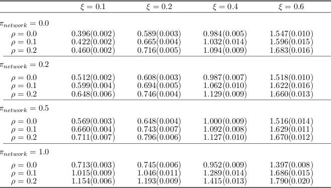
Moreover, we examine the robust aspect of the proposed sSVD with respect to the degree of smoothness of ratings in a neighborhood and the degree of sparseness of a user-specific network. Specifically, givenK = 6 andπ = 0.95, we contaminate the neighborhood structure by increasing the noise level ξ = 0.1,0.2,0.4,0.6, and allow the sparsity ratio πnetwork = 0.0,0.2,0.5,1.0 for user-item specific networks, where the sparseness ratio is the probability that the edges connecting each pair of users or items are removed from the original network. Thus as πnetwork increases, the resultant network becomes sparser, and the proposed sSVD degenerates to rSVD when πnetwork = 1.0. As suggested by Table 2, the performance of sSVD deteriorates as the contamination level πnetwork escalates, yet still outperforming rSVD when ξ = 0.1,0.2. On the other hand, rSVD outperforms the proposed sSVD when ξ ≥ 0.4, which is anticipated because the proposed sSVD relies on the smoothness structure of the ratings. Moreover, it is evident that the proposed sSVD is less affected by the “cold-start” users and items whenπnetwork decreases.

Table 2: Averaged RMSEs and estimated standard deviations over 50 simulations for the proposed method when the error standard deviation is 0.1, 0.2, 0.4, or 0.6, and the “cold-start” rate ρ is 0.0, 0.1, or 0.2, and the network structure missing rateπnetwork is 0.0, 0.2,

0.5, or 1.0.

ξ= 0.1 ξ= 0.2 ξ= 0.4 ξ= 0.6

πnetwork= 0.0

ρ= 0.0 0.396(0.002) 0.589(0.003) 0.984(0.005) 1.547(0.010)

ρ= 0.1 0.422(0.002) 0.665(0.004) 1.032(0.014) 1.596(0.015)

ρ= 0.2 0.460(0.002) 0.716(0.005) 1.094(0.009) 1.683(0.016)

πnetwork= 0.2

ρ= 0.0 0.512(0.002) 0.608(0.003) 0.987(0.007) 1.518(0.010)

ρ= 0.1 0.599(0.004) 0.694(0.005) 1.062(0.010) 1.622(0.016)

ρ= 0.2 0.648(0.006) 0.746(0.004) 1.129(0.009) 1.660(0.013)

πnetwork= 0.5

ρ= 0.0 0.569(0.003) 0.648(0.004) 1.000(0.009) 1.516(0.014)

ρ= 0.1 0.660(0.004) 0.743(0.007) 1.092(0.008) 1.629(0.011)

ρ= 0.2 0.711(0.007) 0.796(0.006) 1.127(0.010) 1.670(0.012)

πnetwork= 1.0

ρ= 0.0 0.713(0.003) 0.745(0.006) 0.952(0.009) 1.397(0.008)

ρ= 0.1 1.015(0.009) 1.046(0.011) 1.289(0.014) 1.686(0.015)

ρ= 0.2 1.154(0.006) 1.193(0.009) 1.415(0.013) 1.790(0.020)

5.2. Music data from Last.fm

In this section, we analyze a online music dataset from theLast.fm (http://www.last.fm), which was released in the second International Workshop HetRec 2011 (http://ir.ii. uam.es/hetrec2011). This dataset contains user-artist listening counts, social networks among 1,892 users, and tagging information for 17,632 artists. The user-artist listening counts contain 92,834 tuples defined by [user, artist, listeningCount], where each user listens to an average of about 49 artists, and each artist has been listened to by about 5 users on average. Note that the observation rate in this dataset is below 0.28%, leading to a severe “cold-start” problem.

For this application, we focus on utilizing user-item specific covariates and networks to solve the “cold-start” issue. Specifically, in the Last.fm dataset, a user-specific social network is available based on 12,717 bi-directional user friendships with an average of about 13 friends per user. Moreover, there are 186,479 tags given by users to artists, with an average of about 99 tags per user, and about 15 tags per artist. A typical tag of an artist gives a short description of the artist, such as “rock”, “electronic”, “jazz” and “80s”. The artist-specific tags are converted to al-length 0/1 covariate vector to indicate whether music tags are assigned to an artist by users, where l is the total number of different tags.

Figure 2 illustrates the listening pattern, showing that a log-transformation of the lis-tening counts appears to be normally distributed. In addition, Figure 3 indicates that only a small portion of artists are popular and frequently listened to by many users. However, the majority of the artists are categorized in more specialized genres, which make them less popular over all, but still having their own followers. This is illustrated by the horizontal and diagonal stripes in Figure 3 respectively.

(a) Original listening counts (b) log-transformed listening counts

Figure 2: The original and log-transformed listening counts in theLast.fm dataset.

Figure 4 shows that popular artists tend to be listened to more by each follower; that is, the number of users listening to each artist is positively related with its averaged listen-ing counts, indicatlisten-ing that misslisten-ing is non-ignorable and that the misslisten-ing pattern shall be incorporated in the recommender system.

Figure 3: Two-dimensional histogram plot of the joint distribution of the observed user-artist pairs from the Last.fm dataset. The grey level represents the concentration, with darker color indicating more densely populated. Together with the joint distribution, the marginal distributions for user and artist are displayed along the horizontal and vertical axes.

covariate effects from user-specific social networks and artist-specific tags. Furthermore, to incorporate the non-ignorable missing pattern, the missing percentage is used to generate 12 homogeneous subgroups of users and 10 homogeneous subgroups of artists for gSVD, and covariates (xu,xi) for sSVD are obtained from 5%, 25%, 50%, 75%, and 95% quantiles of the log observed listening counts in the training set for each user and artist. Also, we slightly modify the weight ωui,u0_i0 defined in (5) using thresholding. Specifically, Sui

u0_i0 = S_uu0S_ii0, where S_uu0 = 0.8 if user u and u0 are adjacent in the user social network, and S_uu0 = 0.5 otherwise; and S_ii0 is computed based on the cosine similarity between the tag information of artistsiand i0. For new users or artists, only user social network and artist tags information are available, therefore the weight function for covariate is automatically set as one. Furthermore, we apply a Gaussian kernel with window size h as the median distance among all user-artist pairs. For each user-artist pair (u, i), we compute the weights as in (5), and truncate them to keep only the five most similar user-artist pairs for each (u, i) to facilitate computation.

For evaluation, we apply 5-fold cross-validation over a random partition of the original dataset, and calculate the RMSE as in Koyejo and Ghosh (2011). For SVD-based methods, we setK= 5, and select the optimalλfrom{1,· · ·,25}through the 5-fold cross-validation. For CRBM, the parameters are set as suggested in Nguyen and Lauw (2016); and for SSR, the parameters are determined through cross-validation as suggested in Zhao et al. (2016).

Table 3: RMSEs of various methods and their estimated standard deviations in parentheses for observed, cold-start, and entire pairs on the Last.fm dataset. Here RBM, SoftImput, SSR, rSVD, gSVD, sSVD denote: restricted Boltzmann machines (Salakhutdinov et al., 2007), SoftImput method (Hastie et al., 2015), Self-recovered side regression (Zhao et al., 2016), regularized SVD method (Paterek, 2007), group-specific SVD method (Bi et al., 2017) and the proposed method, respectively. The second column indicates what type of covariates are used by each method, where N, T and M denote user-specific social networks, artist tags and non-ignorable missing pattern, respectively. The best performance in each setting is bold-faced.

Covariate Observed pair “Cold-start” pair Entire pair

Regression N, T 1.507(.005) 1.832(.023) 1.552(.005)

CRBM N, T 1.507(.005) 1.834(.023) 1.552(.004)

SoftImpute N, T 1.308(.005) 1.832(.023) 1.386(.004)

SSR N, T 1.436(.006) 1.841(.035) 1.493(.009)

rSVD N, T 1.124(.006) 1.832(.023) 1.237(.004)

gSVD M, T 0.997(.013) 1.202(.012) 1.026(.011)

sSVD N, M, T 0.880(.004) 0.706(.003) 0.860(.003)

Table 3 shows that sSVD significantly outperforms its competitors with a RMSE of 0.860 for the entire dataset, whereas gSVD is the second best performer with a RMSE of 1.020. As a reference, these two RMSEs are both smaller than 1.071 for the weighted interaction method under the same setting, which is reported as the best performer in analyzing the

respectively. For the “cold-start” pairs, sSVD yields a more than 40% improvement over the second-best competitor gSVD. Note that SoftImput and rSVD do not perform well in handling the “cold-start” problem, as their penalization leads to the same performance as the regression approach.

6. Summary

This article proposes a smooth collaborative recommender system which integrates the net-work structure of user-item pairs to improve prediction accuracy. The proposed method provides a flexible framework to exploit the covariate information, such as user demograph-ics, item contents, and social network information for users and/or items. The network structure allows us to increase the effective sample size for higher prediction accuracy, in addition to producing a more accurate recommender system for “cold-start” pairs. In addi-tion, we implement a “divide-and-conquer” type of alternating least square algorithm. We also establish the asymptotic properties of the proposed method, which provide the theoret-ical foundation of its superior performance over other state-of-the-art methods. Although the proposed method is formulated based on the latent factor model, the framework can be extended to other models, such as Koren (2008) and Bi et al. (2017).

Acknowledgments

Appendix: technical proofs

Proof of Lemma 1. By the definition of ( ˆP,Qˆ) as a minimizer of (3), we have

( ˆP,Qˆ) = argmin P,Q

1 nm n X u=1 m X i=1 _X

(u0_,i0_)∈Ω

ωui,u0_i0(r_u0_i0 −pT

uqi)2

+λ1

n X

u=1

J(pu) +λ2

m X

i=1 J(qi)

= argmin P,Q

1 nm n X u=1 m X i=1 X

(u0_,i0_)∈Ω

ωui,u0_i0r2_u0_i0 −

X

(u0_,i0_)∈Ω

2ωui,u0_i0r_u0_i0pT_uq_i

+ X

(u0_,i0_)∈Ω

ωui,u0_i0(pT_uq_i)2

+λ1

n X

u=1

J(pu) +λ2

m X

i=1 J(qi)

= argmin P,Q

1 nm n X u=1 m X i=1 X

(u0_,i0_)∈Ω

ωui,u0_i0r2_u0_i0 −

X

(u0_,i0_)∈Ω

2ωui,u0_i0r_u0_i0pT_uq_i+ (pT_uq_i)2

− X

(u0_,i0_)∈Ω

ωui,u0_i0r_u20_i0+

X

(u0_,i0_)∈Ω

ωui,u0_i0r_u0_i02

+λ1

n X

u=1

J(pu) +λ2

m X

i=1 J(qi)

= argmin P,Q

1 nm n X u=1 m X i=1 X

(u0_,i0_)∈Ω

ωui,u0_i0r_u0_i02−

X

(u0_,i0_)∈Ω

2ωui,u0_i0r_u0_i0pT_uq_i+ (pT_uq_i)2

+λ1

n X

u=1

J(pu) +λ2

m X

i=1 J(qi)

= argmin P,Q

1 nm n X u=1 m X i=1 X

(u0_,i0_)∈Ω

ωui,u0_i0r_u0_i0 −pT_uq_i

2 +λ1

n X

u=1

J(pu) +λ2

m X

i=1 J(qi),

where the third equality follows thatP

(u0_,i0_)∈Ωω_ui,u0_i0 = 1 and the fact that adding constants to the cost function does not impact minimization. This completes the proof.

Proof of Theorem 1. Our treatment for bounding P RMSE(θˆ,θ) ≥ η is to bound empirical processes induced by RMSE(·,·) by a chaining argument as in (Wong and Shen, 1995; Shen et al., 2003; Liu and Shen, 2006).

Let Γ(L, η) ={θ ∈ Γ(L) : RMSE(θ,θ0) ≥η} be a parameter subset of the parameter space Γ(L). LetλJ(θ) =λ1Pnu=1J(pu) +λ2Pmi=1J(qi) be the regularizer.

Note that θˆis a minimizer of L(P,Q) inΓ(L), we have that P RMSE(θˆ,θ0))≥η≤

P∗

sup_θ∈Γ(L,η)(L(P0,Q0)− L(P,Q))≥0

, whereP∗ is the outer probability (Billingsley, 2013). Using the expression ofL(P,Q), we obtain an upper bound of the latter as follows.

P∗

sup θ∈Γ(L,η)

(nm)−1X u,i

X

(u0_,i0_)∈Ω

ωui,u0_i0(θ_ui−θ_ui0 )(2r_u0_i0−θ_ui0 −θ_ui) +λJ(θ0)−λJ(θ)≥0

≤P∗

sup θ∈Γ(L,η)

(nm)−1X u,i

X

(u0_,i0_)∈Ω

ωui,u0_i0(θ_ui−θ_ui0 )(2r_u0_i0−θ0_ui−θ_ui)≥ −λJ(θ0)

,

where the fact that λJ(θ) ≥ 0 has been used. Now, let Aj =

θ ∈ Γ(L) : 2j−1η ≤ RMSE(θ,θ0) ≤2jη ;j = 1,· · · ,∞ be a partition in that Γ(L, η) =S∞

the above inequalities, we have thatP RMSE(θˆ,θ0)≥η

is bounded by

∞ X j=1 P∗ sup Aj

(nm)−1X u,i

X

(u0_,i0_)∈Ω

ωui,u0_i0(θ_ui−θ0_ui)(2r_u0_i0 −θ0_ui−θ_ui)≥ −λJ(θ0)

≡

∞

X

j=1 Ij.

Next, we bound each Ij separately. Since P_(u0_,i0_)∈Ωω_ui,u0_i0 = 1,

(nm)−1X u,i

X

(u0_,i0_)∈Ω

ωui,u0_i0(θ_ui−θ0_ui)(2r_u0_i0 −θ0_ui−θ_ui)

= (nm)−1X u,i

X

(u0_,i0_)∈Ω

2ωui,u0_i0(θ_ui−θ_ui0 )(θ0_u0_i0 −θ0_ui)

+(nm)−1X u,i

X

(u0_,i0_)∈Ω

2ωui,u0_i0(θ_ui−θ_ui0 )_u0_i0−(nm)−1

X

u,i

(θui−θ0ui)2,

which, by Assumption A and the fact that ωui,u0_i0 = 0 whenSui

u0_i0 = 0, is upper-bounded by

c1

√

K(nm)−1X u,i

|θui−θ0ui| X

(u0_,i0_)∈Ω

2ωui,u0_i0kx_u0_i0−x_uikα₂

+ (nm)−1X u,i

X

(u0_,i0_)∈Ω

2ωui,u0_i0(θ_ui−θ_ui0 )_u0_i0−(nm)−1

X

u,i

(θui−θ0ui)2.

Then for anyθ∈Aj, (2jη)2 ≥(nm)−1Pu,i(θui−θui0 )2 ≥(2j−1η)2, by the Cauchy-Schwarz inequality,

sup Aj

c1

√

K(nm)−1X u,i

|θui−θ0ui| X

(u0_,i0_)∈Ω

2ωui,u0_i0kx_u0_i0−x_uikα 2 ≤sup Aj c1 √ K

(nm)−1X u,i

(θui−θui0 )2 1/2

(nm)−1X u,i

X

(u0_,i0_)∈Ω

2ωui,u0_i0kx_u0_i0−x_uikα₂2

1/2

≤2c1

√

Kκ12jη.

Thus,Ij ≤P∗

sup_Aj(nm)−1P u,i

P

(u0_,i0_)∈Ω2ω_ui,u0_i0(θ_ui−θ0

ui)u0_i0 ≥(2j−1η)2−2c₁

√

Kκ12jη− λJ(θ0)

. Note thatλJ(θ0)≤η2/4 and RMSE(θ,θ0) =

P

u,i(θui−θui0 )2 1/2

θ∈Aj. For anyη≥24c1

√

Kκ1, (2j−1η)2−2c1

√

Kκ12jη−λJ(θ0)≥22j−4η2, implying that Ij ≤P∗

sup

Aj

(nm)−1X u,i

(θui−θ0ui) X

(u0_,i0_)∈Ω

ωui,u0_i0_u0_i0 ≥22j−4η2

≤P∗sup Aj

(nm)−1 X u,i

(θui−θui0 )2

1/2 _X u,i

X

(u0_,i0_)∈Ω

ωui,u0_i0_u0_i02

1/2

≥22j−4η2

≤P∗

(nm)−1X u,i

X

(u0_,i0_)∈Ω

ωui,u0_i0_u0_i02

1/2

≥2j−4η

≤P∗

max u,i X

(u0_,i0_)∈Ω

ωui,u0_i0_u0_i0≥2j−4η

≤X

u,i

2 exp− 2

(2j−8)_η2

2σ2P

(u0_,i0_)∈Ωω2(x_ui,x_u0_i0)

≤2nmexp−2

(2j−8)_η2

2σ2_κ 2

,

where the second to the last inequalities follow from the Chernoff inequality of a weighted sub-Gaussian distribution (Chung and Lu, 2006) and Assumption B. Hence, there exist some positive constantsa2 and a3, forη≥24c1

√

Kκ1 such that

P RMSE(θˆ,θ0)≥η≤4nm ∞

X

j=1

expn− 2

(2j−8)_η2

2σ2_κ 2

o

≤4nmexp{−a2 η2 σ2_κ 2

}/(1−exp{−a2 η2 σ2_κ

2

})≤a3exp

−a2

η2 σ2_κ

2

+ log(nm) .

The desired result then follows immediately.

Proof of Corollary 1. It suffices to compute κ1 and κ2. First, we will show that for any xui∈ X, when |Ω|is sufficiently large, there exist positive constants a4–a7 such that

X

(u0_,i0_)∈Ω

K_h(kxu0_i0−x_uik₂)Sui

u0_i0 ≥

|Ω|

2 E Kh(kx−xuik2)S ui

∆ = 1

= |Ω| 2 P(S

ui_{= 1|∆ = 1)E K}

h(kx−xuik2)

Sui= 1,∆ = 1

≥a4|Ω|E Kh(kx−xuik2)

Sui= 1,∆ = 1

≥a5|Ω|

Z

K_h(u)f_Uui_|Sui_=1,∆=1(u)du≥a₆|Ω|h Z

K(u)du

≥a7|Ω|h,

where thef_Uui_|Sui_=1,∆=1 is the conditional density forUui, the first inequality follows from the law of large numbers, and the third inequality and the third to the last inequalities follow from Assumption C. Similarly, for some positive constantsa8 and a9,

X

(u0_,i0_)∈Ω

K_h(kxui−xu0_i0k₂)kx_ui−x_u0_i0kαSui

u0_i0 ≤2|Ω|E K_h(Uui)(Uui)α|Sui= 1,∆ = 1

= 2|Ω| Z

where the last inequality follows from Assumptions C and D, and

X

(u0_,i0_)∈Ω

K2_h(kxui−xu0_i0k₂)S_uui0_i0 ≤2|Ω|E K2_h(Uui)|Sui= 1,∆ = 1

≤a9|Ω|h.

Combing the above inequalities yields that

X

(u0_,i0_)∈Ω

ω(x0,xu0_i0)kx0,x_u0_i0kα₂ =

P

(u0_,i0_)∈ΩKh(kx0−xu0_i0k₂)kx₀−x_u0_i0kα 2Suui0_i0

P

(u0_,i0_)∈ΩK_h(kx−x_u0_i0k₂)Sui

u0_i0

≤a8hα.

Furthermore,

X

(u0_,i0_)∈Ω

ω2(x0,xu0_i0)≤

P

(u0_,i0_)∈ΩK2_h(kx₀−x_u0_i0k₂)Sui

u0_i0

P

(u0_,i0_)∈ΩK_h(kx−x_u0_i0k₂)Sui

u0_i0

2 ≤

a9 a2₇|Ω|h.

Consequently, κ1 =hα and κ2 = (|Ω|h)−1, then the desired result follows immediately.

References

Deepak Agarwal, Liang Zhang, and Rahul Mazumder. Modeling item-item similarities for personalized recommendations on Yahoo! front page. Annals of Applied Statistics, 5(3): 1839–1875, 2011.

Stephen H Bach, Matthias Broecheler, Bert Huang, and Lise Getoor. Hinge-loss markov random fields and probabilistic soft logic. Journal of Machine Learning Research, 18 (109):1–67, 2017.

Robert M Bell and Yehuda Koren. Scalable collaborative filtering with jointly derived neigh-borhood interpolation weights. In 7th IEEE International Conference on Data Mining (ICDM 2007), pages 43–52. IEEE, 2007.

Xuan Bi, Annie Qu, Junhui Wang, and Xiaotong Shen. A group-specific recommender system. Journal of the American Statistical Association, 112(519):1344–1353, 2017.

Patrick Billingsley. Convergence of probability measures. John Wiley & Sons, 2013.

Daniel Billsus and Michael J Pazzani. User modeling for adaptive news access. User Modeling and User-Adapted Interaction, 10(2-3):147–180, 2000.

David M Blei, Andrew Y Ng, and Michael I Jordan. Latent Dirichlet allocation. Journal of Machine Learning Research, 3(Jan):993–1022, 2003.

Robin Burke. Hybrid recommender systems: Survey and experiments. User Modeling and User-Adapted Interaction, 12(4):331–370, 2002.

Bilian Chen, Simai He, Zhening Li, and Shuzhong Zhang. Maximum block improvement and polynomial optimization. SIAM Journal on Optimization, 22(1):87–107, 2012.

Hsin Chen and Alan F Murray. Continuous restricted Boltzmann machine with an imple-mentable training algorithm. IEE Proceedings-Vision, Image and Signal Processing, 150 (3):153–158, 2003.

Tianle Chen, Yuanjia Wang, Huaihou Chen, Karen Marder, and Donglin Zeng. Targeted local support vector machine for age-dependent classification. Journal of the American Statistical Association, 109(507):1174–1187, 2014.

Fan Chung and Linyuan Lu. Concentration inequalities and martingale inequalities: A survey. Internet Mathematics, 3(1):79–127, 2006.

Aurore Delaigle and Peter Hall. Defining probability density for a distribution of random functions. Annals of Statistics, 38(2):1171–1193, 2010.

¨

Ozg¨ur Demir, Alexey Rodriguez Yakushev, Rany Keddo, and Ursula Kallio. Item-item music recommendations with side information.CoRR, abs/1706.00218, 2017. URLhttp: //arxiv.org/abs/1706.00218.

Jianqing Fan and Irene Gijbels.Local polynomial modelling and its applications: monographs on statistics and applied probability, volume 66. CRC Press, 1996.

Andrey Feuerverger, Yu He, and Shashi Khatri. Statistical significance of the Netflix chal-lenge. Statistical Science, 27(2):202–231, 2012.

Peter Forbes and Mu Zhu. Content-boosted matrix factorization for recommender systems: Experiments with recipe recommendation. In Proceedings of the 5th ACM conference on Recommender Systems, pages 261–264. ACM, 2011.

Jerome H Friedman and Werner Stuetzle. Projection pursuit regression. Journal of the American Statistical Association, 76(376):817–823, 1981.

Quanquan Gu, Jie Zhou, and Chris Ding. Collaborative filtering: Weighted nonnegative matrix factorization incorporating user and item graphs. InProceedings of the 2010 SIAM International Conference on Data Mining, pages 199–210. SIAM, 2010.

Trevor Hastie, Rahul Mazumder, Jason D Lee, and Reza Zadeh. Matrix completion and low-rank svd via fast alternating least squares. Journal of Machine Learning Research, 16(1):3367–3402, 2015.

Thomas Hofmann. Latent semantic models for collaborative filtering. ACM Transactions on Information Systems (TOIS), 22(1):89–115, 2004.

Pigi Kouki, Shobeir Fakhraei, James Foulds, Magdalini Eirinaki, and Lise Getoor. Hyper: A flexible and extensible probabilistic framework for hybrid recommender systems. In

Proceedings of the 9th ACM Conference on Recommender Systems, pages 99–106. ACM, 2015.

Oluwasanmi Koyejo and Joydeep Ghosh. A kernel-based approach to exploiting interaction-networks in heterogeneous information sources for improved recommender systems. In

Proceedings of the 2nd International Workshop on Information Heterogeneity and Fusion in Recommender Systems, pages 9–16. ACM, 2011.

Ken Lang. Newsweeder: Learning to filter netnews. InProceedings of the 12th International Conference on Machine Learning, pages 331–339, 1995.

Huazhen Lin, Lixian Pan, Shaogao Lv, and Wenyang Zhang. Efficient estimation and computation for the generalised additive models with unknown link function. Journal of Econometrics, 2017.

Greg Linden, Brent Smith, and Jeremy York. Amazon.com recommendations: Item-to-item collaborative filtering. IEEE Internet Computing, 7(1):76–80, 2003.

Yufeng Liu and Xiaotong Shen. Multicategoryψ-learning. Journal of the American Statis-tical Association, 101(474):500–509, 2006.

Shujie Ma and Jian Huang. A concave pairwise fusion approach to subgroup analysis.

Journal of the American Statistical Association, 112(517):410–423, 2017.

JS Marron and WJ Padgett. Asymptotically optimal bandwidth selection for kernel density estimators from randomly right-censored samples. Annals of Statistics, pages 1520–1535, 1987.

Judith Masthoff. Group recommender systems: Combining individual models. In Recom-mender systems handbook, pages 677–702. Springer, 2011.

Prem Melville, Raymond J Mooney, and Ramadass Nagarajan. Content-boosted collabo-rative filtering for improved recommendations. AAAI/IAAI, 23:187–192, 2002.

Stuart E Middleton, Nigel R Shadbolt, and David C De Roure. Ontological user profiling in recommender systems. ACM Transactions on Information Systems (TOIS), 22(1):54–88, 2004.

Bradley N Miller, Istvan Albert, Shyong K Lam, Joseph A Konstan, and John Riedl. Movielens unplugged: Experiences with an occasionally connected recommender system. In Proceedings of the 8th International Conference on Intelligent User Interfaces, pages 263–266. ACM, 2003.

A Mukherjee, K Chen, N Wang, and J Zhu. On the degrees of freedom of reduced-rank estimators in multivariate regression. Biometrika, 102(2):457–477, 2015.

Trong T Nguyen and Hady W Lauw. Representation learning for homophilic preferences. In Proceedings of the 10th ACM Conference on Recommender Systems, pages 317–324. ACM, 2016.

Arkadiusz Paterek. Improving regularized singular value decomposition for collaborative filtering. In Proceedings of KDD Cup and Workshop, pages 5–8, 2007.

Michael J Pazzani, Jack Muramatsu, Daniel Billsus, et al. Syskill & Webert: Identifying interesting web sites. InAAAI/IAAI, volume 1, pages 54–61, 1996.

Matthew Richardson and Pedro Domingos. Markov logic networks. Machine Learning, 62 (1-2):107–136, 2006.

Ruslan Salakhutdinov and Andriy Mnih. Bayesian probabilistic matrix factorization us-ing markov chain monte carlo. In Proceedings of the 25th International Conference on Machine Learning, pages 880–887. ACM, 2008.

Ruslan Salakhutdinov, Andriy Mnih, and Geoffrey Hinton. Restricted Boltzmann machines for collaborative filtering. InProceedings of the 24th International Conference on Machine learning, pages 791–798. ACM, 2007.

David W Scott. Multivariate density estimation: theory, practice, and visualization. John Wiley & Sons, 2015.

Xiaotong Shen, George C Tseng, Xuegong Zhang, and Wing Hung Wong. Onψ-learning.

Journal of the American Statistical Association, 98(463):724–734, 2003.

Nathan Srebro, Noga Alon, and Tommi S Jaakkola. Generalization error bounds for collab-orative prediction with low-rank matrices. In Advances in Neural Information Processing Systems, pages 1321–1328, 2005.

Charles J Stone. An asymptotically optimal window selection rule for kernel density esti-mates. Annals of Statistics, pages 1285–1297, 1984.

Robert Tibshirani and Trevor Hastie. Local likelihood estimation. Journal of the American Statistical Association, 82(398):559–567, 1987.

Philippe Vieu. Nonparametric regression: optimal local bandwidth choice. Journal of the Royal Statistical Society. Series B (Methodological), pages 453–464, 1991.

Larry Wassermann. All of nonparametric statistics. New York: Springer, 2006.

Wing Hung Wong and Xiaotong Shen. Probability inequalities for likelihood ratios and convergence rates of sieve MLEs. Annals of Statistics, 23(2):339–362, 1995.

Feipeng Zhao and Yuhong Guo. Learning discriminative recommendation systems with side information. In Proceedings of the 26th International Joint Conference on Artificial Intelligence, pages 3469–3475, 2017.

Feipeng Zhao, Min Xiao, and Yuhong Guo. Predictive collaborative filtering with side information. In Proceedings of the 25th International Joint Conference on Artificial In-telligence, pages 2385–2391, 2016.

Tinghui Zhou, Hanhuai Shan, Arindam Banerjee, and Guillermo Sapiro. Kernelized prob-abilistic matrix factorization: Exploiting graphs and side information. In Proceedings of the 2012 SIAM International Conference on Data Mining, pages 403–414. SIAM, 2012.