Bayesian Tensor Regression
Rajarshi Guhaniyogi∗ [email protected]
Department of Applied Mathematics & Statistics University of California
Santa Cruz, CA 95064, USA
Shaan Qamar∗ [email protected]
Google Inc.
Mountain View, CA 94043, USA
David B. Dunson [email protected]
Department of Statistical Science Duke University
Durham, NC 27708-0251, USA
Editor:Robert McCulloch
Abstract
We propose a Bayesian approach to regression with a scalar response on vector and ten-sor covariates. Vectorization of the tenten-sor prior to analysis fails to exploit the structure, often leading to poor estimation and predictive performance. We introduce a novel class of multiway shrinkage priors for tensor coefficients in the regression setting and present posterior consistency results under mild conditions. A computationally efficient Markov chain Monte Carlo algorithm is developed for posterior computation. Simulation studies illustrate substantial gains over existing tensor regression methods in terms of estimation and parameter inference. Our approach is further illustrated in a neuroimaging application.
Keywords: Multiway Shrinkage Prior, Magnetic Resonance Imaging (MRI), Parafac Decomposition, Posterior Consistency, Tensor Regression
1. Introduction
In many application areas, it is common to collect predictors that are structured as a multiway array or tensor. For example, the elements of this tensor may correspond to voxels in a brain image (Lindquist, 2008; Lazar, 2008; Hinrichs et al., 2009; Ryali et al., 2010). Existing approaches for quantifying associations between an outcome and such tensor predictors mostly fall within two groups. The first approach assesses the association between each cell (for brain images referred to as voxel) and the response independently, providing a p-value ‘map’ (Lazar, 2008). The p-values can be adjusted for multiple comparisons to identify ‘significant’ sub-regions of the tensor. Although this approach is widely used and appealing in its simplicity, clearly such independent screening approaches have key disadvantages relative to methods that take into account the joint impact of the overall
. ∗These authors contributed equally
c
tensor simultaneously. Unfortunately, the literature on simultaneous analysis approaches is sparse.
One naive approach is to simply vectorize the tensor and then use existing methods for high-dimensional regression. Such vectorization fails to preserve spatial structure, making it more difficult to learn low-dimensional relationships with the response. Efficient learning is of critical importance, as the sample size is typically massively smaller than the total number of cells. Alternative approaches within the regression framework include functional regression and two stage approaches. The former views the tensor as a discretization of a continuous functional predictor. Most of the literature on functional predictors focuses on 1D functions; Reiss and Ogden (2010) consider the 2D case, but substantial challenges arise in extensions to 3D due to dimensionality and collinearity among cells. Recently Wang et al. (2014) considered 3D regularized functional regression with Haar wavelet basis. The article is essentially frequentist in nature with simulation studies showing only the mean squared error and the percentage of correctly identified zero and nonzero elements. Additionally, the article reveals that functional regression is largely affected by the choice of proper basis functions. The second set of approaches, i.e. Two stage approaches first conduct a dimension reduction step, commonly using PCA, and then fit a model using lower dimensional predictors (Caffo et al., 2010). A clear disadvantage of such approaches is that the main principal components driving variability in the random tensor may have relatively limited impact on the response variable. Potentially, supervised PCA could be used, but it is not clear how to implement such an approach in 3D or higher dimensions.
Zhou et al. (2013) propose extending generalized linear regression to include a tensor structured parameter corresponding to the measured tensor predictor. To circumvent diffi-culties with extensions to higher order tensor predictors, they impose additional structure on the tensor parameter, supposing it decomposes as a rank-R parafac sum (see Section 2.1). This massively reduces the effective number of parameters to be estimated. They develop a penalized likelihood approach where adaptive lasso penalties are be imposed on individual margins of the parafac decomposition, focusing on good point estimation for the tensor parameter. However, their method relies heavily on cross-validation for selecting tuning parameters which are sensitive to the tensor dimension, the signal-to-noise ratio (de-gree of sparsity) and the parafac rank. Given that there is no automatic selection procedure for the tuning parameters provided in Zhou et al. (2013), they have to be fed manually by the end user which is problematic for an unknown tensor regression problem.
individual parameters, and also provides shrinkage towards low rank decomposition of the tensor coefficient. Similarly, Bayesian tensor regression framework proposed in Goldsmith et al. (2014) uses binary indicators to determine whether a cell in the tensor predictor is predictive of the response. For a tensor predictor with 30 ×30 ×30 cells, such an approach requires to update 27000 binary indicators in each MCMC iteration and is deemed unsatisfactory due to mixing issues and poor inference.
Our approach differs from image reconstruction literature as we do not model the distri-bution of the tensorX (Qiu, 2007). There is a considerable recent literature on frequentist tensor modeling in which one typically encounters time series (generally to study social networks or images evolving over time) with response at every time point is an array/tensor (Gerard and Hoff, 2015; Hoff et al., 2015). There is also a Bayesian literature that facilitates joint modeling of a large number of unordered categorical variables (Zhou et al., 2015). Our framework is fundamentally different from these approaches in the sense that these are all unsupervised tensor modeling approach while we propose a framework for supervised tensor
regression. To the best of our knowledge, we are the first to propose a novel multiway
shrinkage prior in Bayesian tensor regression framework (with scalar response on a ten-sor predictor) that accommodates shrinkage of the tenten-sor coefficient for the appropriate identification of important cells in the tensor predictor. Besides, we offer strong posterior consistency results on Bayesian tensor regression framework with multiway shrinkage prior.
Remainder of the manuscript evolves as follows. In Section 2, we propose the basic framework of the tensor regression model with a scalar response, vector predictors and a tensor predictor. Section 3 characterizes desirable criteria for a multiway shrinkage prior and proposes a novel multiway shrinkage prior on the tensor coefficient. Sections 4 and 5 provide theoretical results on the convergence of posterior distribution under the mutiway shrinkage prior and details on posterior computation respectively. Various simulation studies with 2D and 3D tensor predictors are presented in Sections 6 and 7 respectively to study effectiveness of the Bayesian tensor regression under various degrees of sparsity and signal strength. Section 8 is devoted to a real brain connectome data analysis using the proposed Bayesian tensor regression model along with its competitors. The manuscripts ends with a discussion.
2. Tensor Regression
This section provides details on the tensor regression model.
2.1 Basic Notation
Let β1 = (β11, . . . , β1p1)
0 and β
2 = (β21, . . . , β2p2)
0 be vectors of length p
1 and p2,
re-spectively. The vector outer product β1 ◦ β2 is a p1 ×p2 matrix with (i, j)-th entry β1iβ2j. A D-way outer product between vectors βj = (βj1, . . . , βjpj), 1 ≤ j ≤ D, is a p1 × · · · × pD multi-dimensional array denoted B = β1 ◦ β2 ◦ · · · ◦ βD with entries (B)i1,...,iD =
QD
j=1βjij. Define a vec(B) operator as stacking elements of thisD-way tensor
into a column vector of lengthQD
j=1pj. From the definition of outer products, it is easy to see that vec(β1◦β2◦ · · · ◦βD) =βD⊗ · · · ⊗β1. As a higher order generalization of matrix singular value decomposition, Tucker decomposition of a D-way tensor B ∈ ⊗D
often considered. The Tucker decomposition (Kolda and Bader, 2009) can be expressed as
B = R1
X
r1=1 R2
X
r2=1
· · ·
RD
X
rD=1
λr1,...,rDβ
(r1)
1 ◦β (r2)
2 ◦ · · · ◦β (rD)
D (1)
where β(jrj) is a pj dimensional vector, 1≤j ≤D, and Λ= (λr1,...,rD)
R1,...,RD
r1,...,rD=1 is referred to as the core tensor. If one considers{β(jrj); 1≤rj ≤Rj,1≤j≤D} as “factor loadings” and λr1,...,rD to be the corresponding coefficients, then the Tucker decomposition may be thought of as a multiway analogue to factor modeling.
A rank-R parafac decomposition emerges as a special case of Tucker decomposition 1 when R1 = R2 = · · · = RD = R and λr1,...,rD = I(r1 = r2 = · · · = rD). In particular, B ∈ ⊗D
j=1<pj assumes a rank-R parafac decomposition if
B = R
X
r=1
β(1r)◦ · · · ◦β(Dr) (2)
where β(jr),1 ≤ j ≤ D and 1 ≤ r ≤ R are the pj dimensional ‘margins’. The parafac decomposition is more widely used due to its relative simplicity.
2.2 Model Framework
Let y ∈ Y denotes a response variable, with z ∈ X ⊂ <p and X ∈ ⊗D
j=1<pj scalar and
tensor predictors, respectively. We consider a tensor regression model having a general form
y∼f α+z0γ+hX,Bi, σ, hX,Bi= vec(X)0vec(B), (3)
wheref(µ, σ) is a family of distributions having locationµand scaleσ,γis ap×1 coefficient for scalar preditors and B ∈ ⊗D
j=1<pj is the tensor parameter corresponding to measured
tensor predictorX. We focus more specifically on the Gaussian linear model case with
y=α+z0γ+hX,Bi+, ∼N(0, σ2). (4) The coefficient tensor B hasQD
j=1pj elements, necessitating substantial dimensionality
reduction. A rank-1 parafac decomposition assumes B = β1 ◦ · · · ◦βD and vec(B) = βD⊗ · · · ⊗β1. This reduces to modelingy=α+z0γ+β01Xβ2 when D= 2, corresponding to the bilinear model considered in Hung and Wang (2013). Since only the single parameter vector βj captures signal along the jth dimension, a rank-1 assumption severely limits flexibility, ruling out interactions among dimensions. Following Zhou et al. (2013), we use a more flexible rank-R parafac decomposition for B =PR
r=1β (r)
1 ◦ · · · ◦β (r)
D introduced in (2) with β(jr)∈ <pj, 1≤j≤D, and 1≤r≤R. Expression (4) then becomes
y=α+z0γ+DX,
R
X
r=1
β(1r)◦ · · · ◦β(Dr)E+
=α+z0γ+ X
(i1,...,iD)
(X)i1,...,iD(B)i1,...,iD+
where voxel (X)i1,...,iD of the tensor predictor has corresponding parameter
(B)i1,...,iD = R
X
r=1 D
Y
j=1
β(j,ijr), (i1, . . . , iD)∈ VB =⊗Dj=1{1, . . . , pj}. (6)
The model is therefore nonlinear in the parameters definingB. A hierarchical specification is completed by placing priors over unknown model parameters. While placing priors over
α and γ is straightforward, Section 3.2 focuses on specification of the prior over tensor parameters which is nontrivial and one of the main contributions of this work.
Under the assumed rank-Rparafac decomposition forB, model (5) requires estimating
p+ 2 +RPD
j=1pj as opposed top+ 2 +QDj=1pj parameters for the unstructured vectorized (saturated) model. As we are interested in identifying geometric sub-regions of the tensor across which coefficients are not close to zero, with the remaining elements being very close to zero, one wonders whether such dramatic dimension reduction retains sufficient flexibility. Finally, we would like to accurately estimate coefficient values in these sub-regions. Consistent with our theoretical analysis in Section 4, extensive simulation studies in Section 6 confirm our ability to accomplish these goals.
2.3 Model Identifiability
From model (5) it is clear that only voxel-level coefficients are identified and not the in-dividual tensor margins defining their product-sum given in (6). In the tensor setting, identifiability restrictions are understood in light of the following indeterminacies:
1. Scale indeterminacy: for each r = 1, . . . , R, define λr = (λ1r, . . . , λDr) such that
QD
j=1λjr = 1. Then replacingβ (r)
j byλjrβ (r)
j leaves the tensor parameterBunaltered.
2. Permutation indeterminacy: PR
r=1◦Dj=1β (r) j =
PR
r=1◦Dj=1β (P(r))
j for any permutation
P(·) of {1,2, . . . , R}. In particular, this implies that◦D j=1β
(r)
j are not identifiable for
r= 1, . . . , R.
3. Orthogonal transformation indeterminacy (D= 2 only): for any orthonormal matrix
O, one has (β(1r)O)◦(β2(r)O) =β1(r)⊗β(2r).
ForD >2, imposing the following (D−1)Rconstraints ensures identifiability of the margin parameters comprising the rank-R parafac decomposition:
3. Multiway Shrinkage Priors
This Section outlines the novel multiway shrinkage prior on the tensor coefficient.
3.1 Vector Shrinkage Priors
There has been recent interest in high-dimensional regression with vector predictors, choos-ing priors which shrink small coefficients towards zero while minimizchoos-ing shrinkage of large coefficients. Many of these priors can be expressed as a global-local (GL) scale mixtures (Polson and Scott, 2012) with
θj ∼N(0, ψjτ), ψj ∼g, τ ∼h, (8)
where (θ1, . . . , θp) is a coefficient vector, τ is a global scale and ψj is a local-scale. When
g is a mixture of two components, with one concentrated near zero and the other away from zero, a spike and slab prior is obtained. Many other choices of g and h have been considered. Although the GL family is widely used and versatile, Bhattacharya et al. (2015) note advantages in drawing the local scales jointly. In particular, they propose to let
θj ∼DE(·|φjτ), (φ1, ..., φp)∼Dirichlet(a, . . . , a), τ ∼h.
where DE(·) denote the double-exponential distribution. For small a and large p, the Dirichlet(a, . . . , a) prior has the property of favoring many values close to zero with a few much larger values, but with P
jφj = 1. Though we draw motivation from literature on vector shrinkage priors, our goal of proposing a shrinkage prior on tensor parameter B is fundamentally more challenging as discussed in forthcoming sections.
3.2 Multiway Priors
We propose a new class of multiway shrinkage priors in the generalized linear model setting with tensor valued predictors. Assuming tensor parameter B admits a rank-R parafac decomposition, model (5) results in cell-level coefficients that are a nonlinear function of the corresponding tensor margin parameters (see (6)). Moreover, this implies simultaneous shrinkage on each of the QD
j=1pj cell coefficients as imposed by the prior over RPDj=1pj parameters. This necessitates careful prior specification on the tensor margins {β(jr); 1 ≤
j≤D,1≤r≤R}such that the induced cell-level prior has adequate tails so as to prevent over shrinkage.
There are a number of desirable characteristics for a multiway prior on the tensor mar-gins. The proposed multiway shrinkage prior must have a structure that facilitates efficient and reliable model fitting. In addition, it is important to ensure that
1. For each r = 1, . . . , R, β1(r,i)
1, . . . , β
(r) D,iD
and β1(r,k)
1, . . . , β
(r) D,kD
are equal in distribu-tion, for any (i1, . . . , iD),(k1, . . . , kD)∈ VB× VBand (i1, . . . , iD)6= (k1, . . . , kD). This is to ensure that (B)i1,...,iD and (B)k1,...,kD have the same distribution apriori.
2. Shrinkage towards a low rank decomposition, with the model adapting to the com-plexity and signal in the data, effectively deleting unnecessary dimensions.
3.3 The Multiway Dirichlet GDP Prior
There are many ways of specifying priors over tensor margins β(jr) to satisfy the crite-ria listed. We propose a particular choice called the multiway Dirichlet generalized
dou-ble Pareto (M-DGDP) prior. This prior induces shrinkage across components in an
ex-changeable way, with global scale τ ∼Ga(aτ, bτ) adjusted in each component as τr =φrτ for r = 1, . . . , R, where Φ = (φ1, . . . , φR) ∼ Dirichlet(α1, . . . , αR) encourages shrink-age towards lower ranks in the assumed parafac decomposition. In addition, Wjr = diag(wjr,1, . . . , wjr,pj), j = 1, . . . , D and r = 1, . . . , R are margin-specific scale parameters for each component. The hierarchical margin-level prior is given by
β(jr)∼N 0,(φrτ)Wjr
, wjr,k ∼Exp(λ2jr/2), λjr ∼Ga(aλ, bλ). (9)
Collapsing over element-specific scales, notice thatβj,k(r)|λjr, φr, τ iid
∼DE(λjr/
√
φrτ), 1≤k≤
pj. Prior (9) induces a GDP prior on the individual margin coefficients which in turn has the form of an adaptive Lasso penalty (Armagan et al., 2013a). Flexibility in estimating Br = {β(jr); 1 ≤ j ≤ D} is accommodated by modeling within-margin heterogeneity via element-specific scaling wjr,k. Common rate parameter λjr shares information between margin elements, encouraging shrinkage at the local scale.
The framework adpoted by Zhou et al. (2013) for Frequentist tensor regression starts by assuming the true parafac rank and relying on shrinkage through a global parameter for estimating the tensor coefficient. In contrast, M-DGDP prior proposes joint shrinkage on the global and local component parameters to achieve improved inference and estimation. Though rank-selection is not our purview, our prior also accomodates dimension reduction by favoring low-rank factorizations as discussed below.
4. Posterior Consistency for Tensor Regression
This Section details out theoretical properties of the tensor regression framework.
4.1 Notation and Framework
We establish convergence results for tensor regression model (5) under the simplifying as-sumptions that the intercept is omitted by centering the response and the error variance is
σ2 = 1. Since our main focus is on the tensor coefficient, we assume coefficients for ordinary scalar covariates to be known. Without loss of generality, we assume γ = (0, . . . ,0). We consider an asymptotic setting in which the dimensions of the tensor grow with n. This paradigm attempts to capture the fact that tensor dimension Q
jpj,n is typically substan-tially larger than sample size. This creates theoretical challenges, related to (but distinct from) those faced in showing posterior consistency for high dimensional regression (Armagan et al., 2013b) and multiway contingency tables (Zhou et al., 2015).
Suppose the data generating model comes from the same class of models where the fitted model belongs to, i.e., having true tensor parameter B0n∈ ⊗D
rank-R PARAFAC decomposition as below
B0n= R
X
r=1
β0(1,nr)◦ · · · ◦β0(D,nr), βj,n0(r)= (βj,n,0(r)1, . . . , βj,n,pj,n0(r) )0 ∈ <pj,n.
In addition, define Fn,F0n∈ <
RPDj=1pj,n
as the vectorized parameters:
Fn= vec β(1)1,n,· · ·,β (R) 1,n,· · ·,β
(1)
D,n,· · ·,β (R) D,n
Fn0 = vec β0(1)1,n ,· · ·,β10(,nR),· · ·,β0(1)D,n,· · ·,β0(D,nR)
.
Define a Kulback-Leibler (KL) neighborhood around the true tensorB0n as
Bn=
(
Bn: 1
n
n
X
i=1
KL(f(yi|B0n), f(yi|Bn))<
)
.
Denote KL(f(yi|B0n), f(yi|Bn)) as KLi. The KL-distance between N(µ1, σ12) and N(µ2, σ22)
is log(σ2/σ1)+ σ12+(µ1−µ2)2
/2σ2
2−12, so it follows KLi= KL N hXi,Bni,1
,N hXi,B0ni,1
= 12 hXi,B0ni − hXi,Bni
2
. Hence, a KL neighborhood of radiusaround B0n can be re-expressed as Bn =
Bn : 21nPni=1 hXi,B0ni − hXi,Bni
2
< . Further, let πn and Πn denote prior and posterior densities withn observations, respectively, and
Πn(Bcn) =
R Bc
nf(yn|Bn)πn(Fn)
R
f(yn|Bn)πn(Fn)
,
with yn = (y1, . . . , yn)0 and f(yn|Bn) is the density of yn under model (5). Posterior consistency is established by showing that
Πn(Bnc)→0 underB0n a.s. asn→ ∞. (10) 4.2 Main Result
Our main theorem is that (10) holds under a simple sufficient condition on the prior and the tensor predictors.
Theorem 1 Let ζn =n 1+ρ3
2 (ρ3 >0), Mn = 1 n
s
n
P
i=1
||Xi||22. Given Lemma 6 in Appendix
A, for any >0, Πn(Bn: n1
Pn
i=1KLi > )→0 a.s. underB0n, for the prior πn(Bn) that
satisfies
πn
Bn:||Bn−B0n||2 <
2η
3Mnζn
>exp(−dn), for all largen (11)
for anyd >0 and η < 32 −d. That is, the model is posterior consistent when (11) holds.
Theorem 2 For fixed constantsH1, H2, M1, ρ1 andρ2>0, the M-DGDP prior (9) onBn
satisfies (11), i.e. yields posterior consistency under conditions:
(a) H1nρ1 < Mn< H2nρ2
(b) supl=1,...,pj,n|βj,n,l0(r)|< M1<∞, for allj = 1, . . . , D, r= 1, . . . , R
(c) PD
j=1pj,nlog(pj,n) =o(n).
Remark 3 Condition (a) in Theorem 2 gives an upper and lower bound on the sum of
the Frobenius norms of tensor predictors. In tensor predictors with {0,1} entries (often
observed for white/grey matter fMRI data), this condition simply imposes a restriction on
the minimum and maximum number of 1s in a tensor predictor as a function of the sample
size n. Condition (b) is mild, assuming the supremum of all entries in the tensor margins
are bounded. Finally, condition (c) in Theorem 2 requires thatP
j=Dpj,n grows sub-linearly
with sample size n. However, note that the number of cellsQD
j=1pj,n in the tensor can grow
at a rate much faster than the sample size n; hence, the modeling framework allows large
tensor covariates even for moderate sample sizes. Of course, condition (c) trivially holds
when the dimension of the tensor is kept fixed as n grows.
Remark 4 Our Section on posterior consistency is based on the assumption that γ = (0, . . . ,0)0 and error variance 1, however the results are trivially extendable to cases with
unknown γ andσ2. In such a generalization, it is important to note that one would need to
assume the dim(γ) is fixed and not growing withn.
4.3 Prior Hyper-parameter Elicitation
The marginal distribution of cell coefficients (6) under the proposed M-DGDP prior (9) is not available in closed-form. To assess how a shrinkage prior on the margins induces prior on cell coefficients of the tensor, we turn to an expression for the cell-level variance:
var(Bi1,...,iD) =E
var
R
X
r=1 D
Y
j=1
β(j,idr) |W,Λ,Φ, τ
=EΦ
R
X
r=1
φDr Eτ{τD}EΛ·,r
EWr|Λr
D
Y
j=1 wjr,ij
= Γ(α0+D) Γ(α0)bDτ
(2Cλ)DEΦ
R
X
r=1 φDr
.
The following Lemma provides lower and upper bounds on the variance that can be useful for elicitation of default hyperparameter values.
Lemma 5 Under M-DGDP shrinkage prior (9) and for D > 1, if α1 = · · · = αR =
c/R, c ∈ N+, with constants Cλ = bλ2/ (aλ −1)(aλ −2)
, aλ > 2, Aτ = exp((D2 − 3D)/2), then the cell-level variance is bounded below by Rα1D(2Cλ/bτ)D and above by
● ● ● ● ● ● ● ● ● ● ● ● ● ● ● ● ● ● ● ● ● ● ● ● ● ● ● ● ● ● ● ● ● ● ● ● ● ● ● ● ● ● ● ●● ● ● ● ● ● ● ● ● ● ● ● ● ● ● ● ● ● ● ● ● ● ● ● ● ● ● ● ● ● ● ● ● ● ● ● ● ● ● ● ● ● ● ● ● ● ● ● ● ● ● ● ● ● ● ●● ● ● ● ● ● ● ● ● ● ● ● ● ● ● ● ● ● ● ● ● ● ● ● ● ● ● ● ● ● ● ● ● ● ● ● ● ● ● ● ● ● ● ● ● ● ● ● ● ● ● ● ● ● ● ● ● ● ● ● ● ● ● ● ● ● ● ● ● ● ● ● ● ● ● ● ● ● ● ● ● ● ● ● ● ● ● ● ● ● ● ● ● ● ● ● ● ● ● ● ● ● ● ● ● ● ● ● ● ● ●● ● ● ● ● ● ● ● ● ● ● ● ● ● ● ● ● ● ● ● ● ● ● ● ● ● ● ● ● ● ● ● ● ● ● ● ● ● ● ● ● ● ● ● ● ● ● ● ● ● ● ● ● ● ● ● ● ● ● ● ● ● ● ● ● ● ● ● ● ● ● ● ● ● ● ● ● ● ● ● ● ● ● ● ● ● ● ● ● ● ● ● ● ● ● ● ● ● ● ● ● ● ● ● ● ● ● ● ● ● ● ● ● ● ● ● ● ● ● ● ● ● ● ● ●● ● ● ● ● ● ● ● ● ● ● ● ● ● ● ● ● ● ● ● ● ● ● ● ● ● ● ● ● ● ● ● ● ● ● ● ● ● ● ● ● ● ● ● ● ● ● ● ● ● ● ● ● ● ● ● ● ● ● ● ● ● ● ● ● ● ● ● ● ● ● ● ● ● ● ● ● ● ● ● ● ● ● ● ● ● ● ● ● ● ● ● ● ● ● ● ● ● ● ● ● ● ● ● ● ● ● ● ● ● ● ● ●● ● ● ● ● ● ● ● ● ● ● ● ● ● ● ● ● ● ● ● ● ● ● ● ● ● ● ● ● ● ● ● ● ● ● ● ● ● ● ● ●●●● ● ● ● ● ● ● ●
(a)α= (0.2,0.2,0.2)
● ● ● ● ● ● ● ● ● ● ● ● ● ● ● ● ● ● ● ● ● ● ● ● ● ● ● ● ● ● ● ● ● ● ● ●● ● ● ● ● ● ● ● ● ● ● ● ● ● ● ● ● ● ● ● ● ● ● ● ● ● ● ● ● ● ● ● ● ● ● ● ● ● ● ● ● ● ● ● ● ● ● ● ● ● ● ● ● ● ● ● ● ● ● ● ● ● ● ● ● ● ● ● ● ● ● ● ● ● ● ● ● ● ● ● ● ● ● ● ● ● ● ● ● ● ● ● ● ● ● ● ● ● ● ● ● ● ● ● ● ● ● ● ● ● ● ● ● ● ● ● ● ● ● ● ● ● ● ● ● ● ● ● ● ● ● ● ● ● ● ● ● ● ● ● ● ● ● ● ● ● ● ● ● ● ● ● ● ● ● ● ● ● ● ● ● ● ● ● ● ● ● ● ● ● ● ● ● ● ● ● ● ● ● ● ● ● ● ● ● ● ● ● ● ● ● ● ● ● ● ● ● ● ● ● ● ● ● ● ● ● ● ● ● ● ● ● ● ● ● ● ● ● ● ● ● ● ● ● ● ● ● ● ● ● ● ● ● ● ● ● ● ● ● ● ● ● ● ● ● ● ● ● ● ● ● ● ● ● ● ● ● ● ● ● ● ● ● ● ● ● ● ● ● ● ● ●● ● ● ● ● ● ● ● ● ● ● ● ● ● ● ● ● ● ● ● ● ● ● ● ● ● ● ● ● ● ● ● ● ● ● ● ● ● ● ●● ● ● ● ● ● ● ●●● ● ● ● ● ● ● ● ● ● ● ● ● ● ● ● ● ● ● ● ● ● ● ● ● ● ● ● ● ● ● ● ● ● ● ● ● ● ● ● ● ● ● ● ● ● ● ● ● ● ● ● ● ● ● ● ● ● ● ● ● ● ● ● ● ● ● ● ● ● ● ● ● ● ● ● ● ● ● ● ● ● ● ● ● ● ●● ● ● ● ● ● ● ● ● ● ● ● ● ● ● ● ● ● ● ● ● ● ● ● ● ● ● ● ● ● ● ● ● ● ● ● ● ● ● ● ● ● ● ● ● ● ● ● ● ● ● ● ● ● ● ●
(b)α= (0.3,0.3,0.3)
● ● ● ● ● ● ● ● ● ● ● ● ● ● ● ● ● ● ● ● ● ● ● ● ● ● ● ● ● ● ● ● ● ● ● ● ● ● ● ● ● ● ● ● ● ● ● ● ● ● ● ● ● ● ● ● ● ● ● ● ● ● ● ● ● ● ● ● ● ● ● ● ● ● ● ● ● ● ● ● ● ● ● ● ● ● ● ● ● ● ● ● ● ● ● ● ● ● ● ● ● ● ● ● ● ● ● ● ● ● ● ● ● ● ● ● ● ● ● ● ● ● ● ● ● ● ● ● ● ● ● ● ● ● ● ● ● ● ● ● ● ● ● ● ● ● ● ● ● ● ● ● ● ● ● ● ● ● ● ● ● ● ● ● ● ● ● ● ● ● ● ● ● ● ● ● ● ● ● ● ● ● ● ● ● ● ● ● ● ● ● ● ● ● ● ● ● ● ● ● ● ● ● ● ● ● ● ● ● ● ● ● ● ● ● ● ● ● ● ● ● ● ● ● ● ● ● ● ● ● ● ● ● ● ● ● ● ● ● ● ● ● ● ● ● ● ● ● ● ● ● ● ● ● ● ● ● ● ● ● ● ● ● ● ● ● ● ● ● ● ● ● ● ● ● ● ● ● ● ● ● ● ● ● ● ● ● ● ● ● ● ● ● ● ● ● ● ● ● ● ● ● ● ● ● ● ● ● ● ● ● ● ● ● ● ● ● ● ● ● ● ● ● ● ● ● ● ● ● ● ● ● ● ● ● ● ● ● ● ● ● ● ● ● ● ● ● ● ● ● ● ● ● ● ● ● ● ● ● ● ● ● ● ● ● ● ● ● ● ● ● ● ● ● ● ● ● ● ● ● ● ● ● ● ● ● ● ● ● ● ● ● ● ● ● ● ●● ● ● ● ● ● ● ● ● ● ● ● ● ● ● ● ● ● ● ● ● ● ● ● ● ● ● ● ● ● ● ● ● ● ● ● ● ● ● ● ● ● ● ● ● ● ● ● ● ● ● ● ● ● ● ● ● ● ● ● ● ● ● ● ● ● ● ● ● ● ● ● ● ● ● ● ● ● ● ● ● ● ● ● ● ● ● ● ● ● ● ● ● ● ● ● ● ● ● ● ● ● ●
(c)α= (0.5,0.5,0.5)
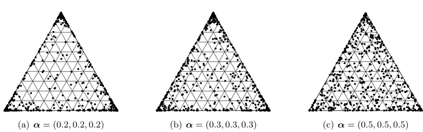
Figure 1: Visualization of points in theS2 probability simplex for 500 independent
realiza-tions of Dirichlet(α). As α ↓ 0, points increasingly tend to concentrate around vertices of theSR−1 simplex. This notion of sparsity is made precise in Yang and
Dunson (2014).
Hyperparameters of the Dirichlet component in multiway prior (9) play a key role in controlling dimensionality of the model, with smaller values favoring more component-specific scales τr ≈0, thus effectively collapsing on a low-rank tensor factorization. Figure 1 plots realizations from the Dirichlet distribution whenR = 3 for different concentration parameters2 α.
A discrete uniform prior is placed on α over a grid, A. By default, grid values are chosen to be 10 equally spaced values in [R−D, R−0.10], letting the data tune this parameter according to the degree of sparisty present. Armagan et al. (2013a) study various choices of (aλ, ζ = bλ/aλ) that lead to desirable shrinkage properties, such as Cauchy-like tails forβj,k(r) while retaining Laplace-like shrinkage near zero. Empirical results from simulation studies across a variety of settings in Section 6 reveal no strong sensitivity to choices for hyper-parameters aλ, bλ. From Lemma 5, setting aλ = 3 and bλ = 2D
√
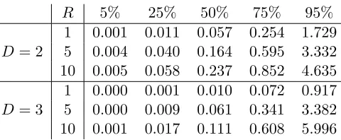
aλ avoids overly narrow variance of the induced prior on tensor elements,Bi1,...,iD. Table 1 provides various quantiles of the induced prior on these elements under these default hyperparameter settings as a function of the parafac rank-R and tensor dimension D.
5. Posterior Computation and Model Fitting
Lettingy ∈ <denote a response, and z ∈ <p,X ∈ ⊗D
j=1<pj predictors, we let y|γ,B, σ∼N z0γ+hX,Bi, σ2
B = R
X
r=1
Br, Br=β1(r)◦ · · · ◦β(Dr)
σ2 ∼πσ, γ∼πγ, β(jr)∼πβ.
(12)
R 5% 25% 50% 75% 95%
D= 2
1 0.001 0.011 0.057 0.254 1.729 5 0.004 0.040 0.164 0.595 3.332 10 0.005 0.058 0.237 0.852 4.635
D= 3
1 0.000 0.001 0.010 0.072 0.917 5 0.000 0.009 0.061 0.341 3.382 10 0.001 0.017 0.111 0.608 5.996
Table 1: Percentiles for |Bi1,...,iD| under the M-DGDP prior with default aλ = 3, bλ = 2D√a
λ,bτ =αR1/D(v = 1) and α = 1/R. Statistics are displayed as the parafac rank-R vary and dimensionD of the tensor vary.
The noise variance is modeled using a conjugate inverse-gamma prior,σ2 ∼IG(v/2, vs20/2), with v= 2 and s20 chosen by default so Pr(σ2 ≤1) = 0.95 assuming a centered and scaled response. Regression coefficients are given a conjugate normal prior γ ∼N(0, σ2Σ0γ) and
the tensor predictor is normalized over all cells to have mean zero and variance 1, allowing one to assume default values for hyper-parameters in the proposed multiway prior.
5.1 Posterior Computation
The proposed multiway prior (9) leads to Gibbs sampling scheme for most parameters of the tensor regression model (12). We rely on marginalization and blocking to reduce auto-correlation for β(jr), wjr; 1≤j ≤D,1≤r ≤R
,(Φ, τ),(γ, σ) , drawing in sequence from [α,Φ, τ|B, W], [B, W|Φ, τ,γ, σ,y] and [γ, σ|B,y] as follows:
(1) Sample [α,Φ, τ|B,W] compositionally as [α|B,W][Φ, τ|α,B,W]:
(a) Sample from the conditional distribution of Dirichlet concentration parameter [α|B,W] via griddy-Gibbs: form a reference set by drawing M samples from [Φ, τ|α,B,W] for each α ∈ A. Set wj,l =π(B|α,Φl, τl,W)π(Φl, τl|α), 1 ≤l≤M,p(α|B,W) =
π(α)PM
l=1wj,l/M, and Pr(α=αj|−) =p(αj|B,W)/
P
α∈Ap(α|B,W).
(b) Sample component-specific scales as [Φ, τ|α∗,B,W] = [Φ|B,W][τ|Φ,B,W]; de-finep0=PDj=1pj, and recallaτ =PrR=1αr =Rαandbτ =α(R/v)1/D (see Section 3.3), then
• draw ψr ∼ giG(α−p0/2,2bτ,2Cr), Cr = PjD=1β(jr)TWjr−1β(jr), and set φr =
ψr/PRl=1ψl in parallel for 1≤r ≤R (see Appendix A for definition of ‘giG’)
• drawτ ∼giG(aτ−Rp0/2,2bτ,2PRr=1Dr),Dr =Cr/φr.
(2) Sample from (β(jr), wjr, λjr); 1≤ j ≤D,1 ≤ r ≤R |Φ, τ,γ, σ,y using a back-fitting procedure to produce a sequence of draws from the margin-level conditional distri-butions across components. For r = 1, . . . , R and j = 1, . . . , D, sample from condi-tional distribution [(β(jr), wjr, λjr)|β(−rj),B−r,Φ, τ,γ, σ,y], where β(−rj) = {β
(r)
l , l 6= j} and B−r=B\Br;
• drawλjr∼Ga aλ+pj, bλ+||β(jr)||1/
√
φrτ
; and
• drawwjr,k ∼giG 12, λ2jr, β 2 (r) j,k /(φrτ)
independently for 1≤k≤pj
(b) drawβ(jr)∼N(µjr,Σjr): defineh(i,j,kr) =Ppd11,...,pD=1,...,dD=1I(dj =k)xd1,...,dD
Q
l6=jβ (r) l,il
,
Hi,j(r) = (h(i,j,r)1, . . . , hi,j,pj(r) )0, ˜yi = yi −z0iγ −
P
l6=rhXi,Bli for 1 ≤ i ≤ n; then Σjr= H(jr)TH
(r)
j /σ2+W
−1 jr/(φrτ)
−1
,µjr=ΣjrH(jr)y˜/σ2
(3) Sample [γ, σ|B,y] = [γ|σ,y˜][σ2|y˜]; define ˜yi =yi− hXi,Bi for 1≤i≤n, then (a) draw σ2∼IG(aσ, bσ), aσ = (n+v)/2,bσ = vs20+||y˜||22−y˜TZµγ
/2
(b) draw γ∼N µγ, σ2Σγ
,Σγ = ZTZ+Σ−0γ1 −1
,µγ =ΣγZTy˜.
6. Simulation Studies
To illustrate finite-sample performance of the proposed multiway priors, we show results from a simulation study with various dimensionality (p, R) and define ¯b = max|B0i1,...,iD|
as the maximum signal size. Throughout, set pj = p, true error variance σ02 = 1 and
¯b = 1 for convenience. In addition, we set the true vector coefficient γ
0 = (0, . . . ,0) and
focus exclusively on inference for tensor parameter B. The following simulated setups are considered:
1. “Generated” tensor: We construct tensor parameters having rank R0 = {3,5} with p={64,100} and D= 2.
2. “Ready made” tensor: We use three tensor (2D) images without generating them from a parafac decomposition with known rank.
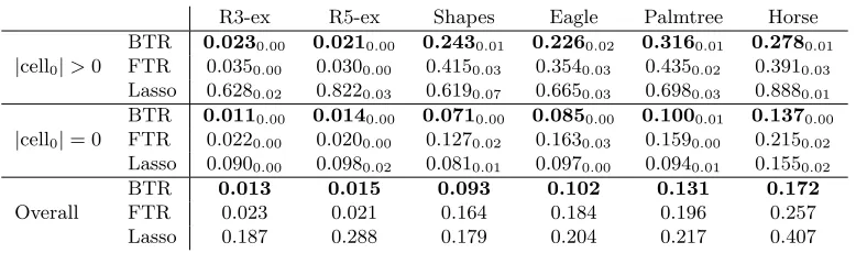
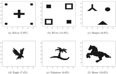
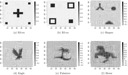
Five replicated datasets with n = 1000 are generated according to (12) with xi1,...,iD ∼ N(0,1). The tensor parameters considered are shown in Figure 2, where the magnitude of the non-zero cells is ¯b = 1. Examples are chosen to demonstrate recovery of cell-level coefficients across varying degrees of complexity (dimension, parafac rank) and sparsity (% of non-zero cells; see Figure 2). The performance of our method with M-DGDP prior (9) (BTR) is compared with (i) frequentist tensor regression with penalization (FTR)(Zhou et al., 2013); and (ii) Lasso (on the vectorized tensor predictor). Comparisons are based on (a) cell mean squared estimation error (true non-zero, true zero, and overall); and (b) frequentist coverage (and length) of 95% credible intervals.
R3-ex R5-ex Shapes Eagle Palmtree Horse
|cell0|>0
BTR 0.0230.00 0.0210.00 0.2430.01 0.2260.02 0.3160.01 0.2780.01
FTR 0.0350.00 0.0300.00 0.4150.03 0.3540.03 0.4350.02 0.3910.03
Lasso 0.6280.02 0.8220.03 0.6190.07 0.6650.03 0.6980.03 0.8880.01
|cell0|= 0
BTR 0.0110.00 0.0140.00 0.0710.00 0.0850.00 0.1000.01 0.1370.00
FTR 0.0220.00 0.0200.00 0.1270.02 0.1630.03 0.1590.00 0.2150.02
Lasso 0.0900.00 0.0980.02 0.0810.01 0.0970.00 0.0940.01 0.1550.02
Overall
BTR 0.013 0.015 0.093 0.102 0.131 0.172
FTR 0.023 0.021 0.164 0.184 0.196 0.257
Lasso 0.187 0.288 0.179 0.204 0.217 0.407
Table 2: Comparison of cell estimation as measured by root mean squared error (RMSE) for the six 2D tensor images portrayed in Figure 2. Results from FTR (Zhou et al., 2013) use R = 10. For BTR, R = 10 is used as an upper bound to the tensor parafac rank. Subscript shows the standard error over a few replicated simulations.
over a grid of values to minimize RMSE for the tensor predictor3. In real applications, cross validation instead would be used to select the tuning parameter that results in lowest hold-out predictive RMSE for FTR. Assuming 10-fold cross validation were used over a vector of 20 tuning parameters, FTR would have a runtime of approximately 8 hours. It also needs to be mentioned that the convergence of parameters in BTR is extremely rapid with an average effective sample size (ESS)≈600 over 1000 iterations.
Cell-level RMSE reported in Table 2 demonstrates that our method (BTR) consistently out performs FTR. When the tensor parameter has a low-rank parafac decomposition (‘R3-ex’ and ‘R5-(‘R3-ex’), BTR and FTR perform best, with BTR having lower RMSE on both true zero and non-zero cells. This validates empirically prior (9) along with our suggested default hyper-parameter choices in Section 3. In particular, the tensor coefficient in BTR has three different types of shrinkage parameters: global, local and shrinkage across ranks. Such a careful construction of shrinkage prior on B adapts to varying degrees of sparsity, shrinking many tensor coefficients close to zero while accurately estimating nonzero cells. FTR shrinkage being dependent on only local parameters suffers in terms of both inferential and predictive performances.
Table 3 demonstrate that BTR yields 95% credible intervals with good frequentist cov-erage across each of the simulated settings, both overall as well as on the true non-zero coefficients. Our method is one of the first to offer uncertainty quantification for tensor valued predictors.Finally, Table 4 provides evidence of the robustness of our method to in-creasing predictor dimension using two of the simulated examples. In both cases, RMSE for FTR worsens considerably on the true zero coefficients. For the true nonzero cells, RMSE increases for both methods as the margin dimension increases; however on a relative basis, FTR worsens considerably more, while on an absolute scale, BTR remains the clear winner.
10 20 30 40 50 60
10
20
30
40
50
60
(a) R3-ex (7.0%)
10 20 30 40 50 60
10
20
30
40
50
60
(b) R5-ex (11.0%)
10 20 30 40 50 60
10
20
30
40
50
60
(c) Shapes (6.8%)
10 20 30 40 50 60
10
20
30
40
50
60
(d) Eagle (7.4%)
10 20 30 40 50 60
10
20
30
40
50
60
(e) Palmtree (8.0%)
10 20 30 40 50 60
10
20
30
40
50
60
(f) Horse (18.6%)
Figure 2: Simulated data with 64×64 2D tensor images (p = 64, D = 2). Row 1: The first two images (from left) have a rank-3 and rank-5 parafac decomposition; the third image is “regular”, although does not have a low-rank parafac decomposi-tion. Row 2: All three images are irregular, and do not have a low-rank parafac decomposition. Sparsity (% non-zero cells) are displayed in sub-captions.
R3-ex R5-ex Shapes Eagle Palmtree Horse
|cell0|>0 coverage 0.9860.02 0.9460.02 0.7470.01 0.7310.04 0.6770.04 0.7950.02
Overall coverage 0.9950.01 0.9700.01 0.9650.00 0.9400.02 0.9480.02 0.9270.01 length 0.0660.01 0.0610.01 0.2900.00 0.3010.03 0.4100.03 0.5660.02
10 20 30 40 50 60
10
20
30
40
50
60
0.1 0.3 0.5 0.7 0.9
(a) R3-ex
10 20 30 40 50 60
10
20
30
40
50
60
0.1 0.3 0.5 0.7 0.9
(b) R5-ex
10 20 30 40 50 60
10
20
30
40
50
60
−0.3 −0.1 0.1 0.3 0.5 0.7 0.9 1.1 1.3
(c) Shapes
10 20 30 40 50 60
10
20
30
40
50
60
−0.2 0 0.2 0.4 0.6 0.8 1 1.2 1.4
(d) Eagle
10 20 30 40 50 60
10
20
30
40
50
60
−0.5 −0.3 −0.1 0.1 0.3 0.5 0.7 0.9 1.1 1.3
(e) Palmtree
10 20 30 40 50 60
10
20
30
40
50
60
−0.6 −0.4 −0.2 0 0.2 0.4 0.6 0.8 1 1.2 1.4
(f) Horse
Figure 3: Recovered images for the 64×64 2D tensor images in Figure 2 using our proposed BTR method. Here,R= 10 is used as an upper bound to the tensor parafac rank.
|cell0| R5-ex Shapes
64 100 64 100
BTR
coverage >0 0.9460.02 0.9910.01 0.7470.01 0.5900.06
length >0 0.0610.01 0.0690.01 0.2900.00 0.2470.01
rmse >0 0.0210.00 0.0320.01 0.2430.01 0.3200.03
rmse = 0 0.0140.00 0.0140.00 0.0710.00 0.0630.00
FTR rmse >0 0.0300.00 0.3690.06 0.4150.03 0.5860.14 rmse = 0 0.0200.00 0.1110.02 0.1270.02 0.1350.02
7. Simulated response with a real 3D brain image
We analyze data containing 3D MRI images for 550 adolescents, with information such as age and sex available. Age and sex are treated as ordinary scalar covariates while 3D MRI images act as tensor covariates. LetX denote a 30×30×30 3D MRI image,Z1be the age and Z2 be the sex of an individual. The response is simulated usingy∼N Z0γ+hX,B0i, σ2
, whereZ denotes (Z1, Z2)0,γ ∈ R2 andB0 ∈ R30×30×30.
We assume the true B0 is a rank 2 tensor, with B0 = a1 ◦a2 ◦ a3 +b1 ◦b2 ◦b3.
Initialization and standardization of predictors follow exactly as prescribed in Section 5. By varyingai’s and bi’s, the following cases with varying degrees of sparsity in the tensor parameterB0 are considered:
Case 1: b1 =b2= (0, . . . ,0,sin((1 : 15)∗π/4)), b3 = (sin((1 : 10)∗π/4),0, . . . ,0),
a1 = (0, . . . ,0,sin((1 : 10)∗π/4)),a2= (0, . . . ,0,cos((1 : 15)∗π/4)),
a3 = (sin((1 : 15)∗π/4),0, . . . ,0).
Case 2: b1 =b2= (0, . . . ,0,sin((1 : 15)∗π/6)), b3 = (sin((1 : 20)∗π/6),0, . . . ,0),
a1 = (0, . . . ,0,sin((1 : 15)∗π/4)),a2= (0, . . . ,0,cos((1 : 10)∗π/6)),
a3 = (sin((1 : 15)∗π/6),0, . . . ,0).
Case 3: b1 =b2= (0, . . . ,0,sin((1 : 20)∗π/6)), b3 = (sin((1 : 20)∗π/6),0, . . . ,0),
a1 = (0, . . . ,0,sin((1 : 10)∗π/4)),a2= (0, . . . ,0,cos((1 : 20)∗π/4)),
a3 = (sin((1 : 20)∗π/6),0, . . . ,0).
We implement BTR, FTR, and Lasso on the vectorized tensor. As before, we present results for FTR withR= 10 (See additional discussion in Section 6 on FTR default setup). Point estimates for coefficients corresponding to age and sex covariates are provided in Table 6. Table 5 summarizes RMSEs for the estimated tensor coefficients for each method. BTR shows at least a 15% improvement over FTR on simulated cases considered. Evidently BTR tends to outperform FTR and vectorized lasso by a greater margin in less sparse settings as well. Importantly, every parameter in BTR is auto-tuned, while the TensorReg
toolbox used for FTR (Zhou et al., 2013) requires calibrating tuning parameter values specific to each setting. Note that rather than using cross validation, tuning parameters in these experiments were chosen to provide the lowest possible (most optimistic) RMSE for the tensor coefficient. FTR fixes R = 10 based on findings discussed in Section 6 while BTR sets R = 10 as an upper bound, concentrating on a lower dimension parafac rank via adaptive shrinkage. While vectorized lasso and FTR do not come equipped with parameter uncertainty estimates, Table 7 demonstrates how BTR consistently provides over 95% coverage across examples with varying degrees of sparsity.
Finally, Table 8 provides a measure of mixing efficiency for a single MCMC run in each of the simulated cases considered (post burn-in over the remaining 1000 MCMC samples). All reported RMSE and coverage statistics were computed over these draws as well (thinning by 5 as previously discussed in Section 6).
8. Brain Connectome Data Analysis
Case 1 Case 2 Case 3
|cell0|>0
BTR 0.39 0.30 0.34
FTR 0.46 0.41 0.43
Lasso 0.46 0.42 0.44
|cell0|= 0
BTR 0.04 0.14 0.10
FTR 0.00 0.00 0.00
Lasso 0.01 0.03 0.02
Overall
BTR 0.13 0.20 0.17
FTR 0.15 0.22 0.18
Lasso 0.15 0.23 0.18
Table 5: Comparison of cell estimation as measured by root mean squared error (RMSE) for the coefficients in case 1,2, 3 corresponding to 3D tensor images. Results from both BTR and FTR (Zhou et al., 2013) use R= 10.
Case 1 Case 2 Case 3
γ1 (truth = 0.5)
BTR 0.57 0.54 0.33
FTR 0.46 0.85 0.95
γ2 (truth = 2.0) BTR 2.00 2.04 1.86
FTR 1.87 0.22 3.30
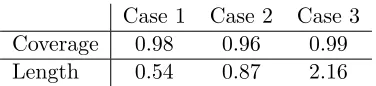
Case 1 Case 2 Case 3
Coverage 0.98 0.96 0.99
Length 0.54 0.87 2.16
Table 7: Length and coverage of 95% credible intervals for BTR. Values are reported as averages over all voxels of the tensor coefficient.
τ2 Scalar predictorγi (Ave.) Tensor predictor βijk (Ave.)
Case 1 (88% sparsity) lag-2 0.04 0.34 0.45
lag-4 0.01 0.11 0.22
Case 2 (82% sparsity) lag-2 0.08 0.33 0.46
lag-4 0.03 0.12 0.23
Case 3 (70% sparsity) lag-2 0.09 0.43 0.53
lag-4 0.02 0.30 0.40
Table 8: MCMC autocorrelation of the proposed BTR method on data studies of Section 7 generated using 3D brain MRI scans.
number of cells in the tensor predictor. In this setting, developing well calibrated predictive models is thus of key importance.
To investigate the performance of competing methods outside the class of fMRI brain image data, we present an analysis using a brain connectome dataset on structural con-nectivity. Data are extracted from diffusion tensor imaging (DTI) and consist of estimates of the number of “fibers” connecting pairs of brain regions for 109 individuals. For each individual, brain connections among 70 brain regions (following desikan atlas) are encoded by a 70×70 weighted adjacency matrix. The (i, j)-th off-diagonal entry in the adjacency matrix is the estimated number of fiber tracts connecting thei-th andj-th brain region. The data also provides 10 clinical covariates for every individual, including sex, age, openness, agreeableness and conscientiousness.
The focus of this study is on developing a predictive model with Creativity Composite Index (CCI) as a response fitted against clinical covariates and a tensor covariate (i.e., the weighted adjacency matrix). Implementing FTR on this data using theTensorReg package was attempted, however, functions in the toolbox require n > R×p. In this example, becausen= 109 andp= 70, it is only possible therefore to fit FTR withR= 1, which has previously been found to perform poorly by Zhou et al. (2013). We therefore compare our proposed method (BTR) to the vectorized Lasso on the basis of their predictive performance. To assess the predictive performance, the sample of n = 109 individuals are divided into 10 folds. Both vectorized lasso and BTR are fitted on 9 folds as training data and the remaining fold as the hold out sample. This is carried out for each of the 10 folds and predictive inferences are obtained for both vectorized lasso and BTR.
Method avg(RMSE) sd(RMSE) avg(cov.) sd(cov.) avg(cor.) sd(cor.)
Lasso 9.21 2.18 63% 20% 0.31 0.11
BTR 9.03 1.64 91% 10% 0.32 0.13
Table 9: mean and standard deviation of RMSEs and cor(yobs, ypred) of Lasso and BTR over 10 folds of the data. It also provides mean and standard deviation of coverages of Lasso and BTR over 10 folds of the data
folds. Given the very high degree of sparsity in the connectome adjacency matrix, it is not surprising that the Lasso is competitive to BTR. However, note that BTR detects this signal with far fewer effective parameters as compared to vectorized lasso. Finally, we measure coverage of 95% predictive intervals for all competitors. The latter is of course a byproduct of our fully Bayesian approach (BTR), while for the Lasso we use a two-staged approach. First we estimate the regression coefficients and subsequently construct approximate 95% predictive intervals based on the normal response-model centered on the predictive mean with variance equal to the estimated residual variance.
9. Discussion
This work develops a novel class of prior distributions on tensor valued predictors which substantially reduces dimensionality relative to vectorizing, providing a multiway analogue of vector shrinkage priors, and enabling high dimensional region selection. The prior on tensor coefficient constructed here imparts shrinkage of the tensor components at global and local levels, while also encouraging shrinkage towards low rank tensor decomposition. In contrast, existing penalization framework on the tensor coefficient shrinks only at the global level. Strong theoretical results are proved for the proposed class of multiway shrink-age priors and a computationally efficient MCMC algorithm is developed in the regression setting. We plan to extend methods developed here to settings where the measured re-sponse for each subject is binary (e.g., indicator of a heath outcome) or multivariate, i.e., y = (y1, ..., yd). Also, the current framework of Bayesian tensor regression fixes rankR of the PARAFAC decomposition at reasonably large value. It might be of interest to learn the PARAFAC rankR by adding a discrete prior distribution onR.
Acknowledgement
The authors would like to thank Joshua T. Vogelstein from Johns Hopkins university for gracefully allowing us to utilize their brain connectome dataset in the real data analysis of our proposed BTR method.
Appendix A
MCMC algorithm
The following derivations concern the M-DGDP prior (9) and the sampling algorithm out-lined in Section 5.1.
For step (1b) Recall from Section 3.3 thatτ ∼Ga(aτ, bτ) and Φ∼Dirichlet(α1, . . . , αR) and denote p0=PDj=1pj. Then,
π(Φ|B,ω) ∝ π(Φ)
Z ∞
0
π(B|ω,Φ, τ)π(τ)dτ
∝ h
R
Y
r=1 φαrr −1
iZ ∞
0 R
Y
r=1
h
(τ φr)−p0/2exp
− 1
τ φr d
X
j=1
||βjr||2/(2ωjr)
i
τaτ−1exp(−bττ)dτ
∝ h
R
Y
r=1 φαr−
p0
2−1
iZ ∞
0
τaτ−R
p0
2 −1 R
Y
r=1
exp
− Cr
τ φr
−bτ(τ φr)
dτ
with Cr =Pdj=1||βjr||2/(2ωjr). Whenaτ =PRr=1αr, this contains the kernel of a gener-alized inverse Gaussian (gIG) distribution for (τ φr). Recall: X ∼fX(x) = giG(p, a, b) ∝
xp−1exp(−(ax+b/x)/2). Following Lemma 9 in the Appendix B, for independent random variableTr ∼fr on (0,∞), the joint density of{φr=Tr/Pr˜Tr˜:r= 1, . . . , R}has support
on SR−1. In particular,
f(φ1, . . . , φR−1) =
Z ∞
0 tR−1
R
Y
r=1
fr(φrt) dt, φR= 1−
X
r<R
φr.
Substituting fr(x) ∝ x−δrexp(−Cr/x) exp(−bτx) in the above expression yields
f(φ1, . . . , φR−1) ∝
Z ∞
0
τR−1
R
Y
r=1
(φrτ)−δrexp
− Cr
(φrτ)
−bτ(φrτ)
dτ
=
hYR
r=1 φ−δr
iZ ∞
0
τR−Prδr−1 R
Y
r=1
exp
− Cr
(φrτ)
−bτ(φrτ)
dτ.
Matching exponents between this expression and the preceding one implies (1)aτ−R(p0/2)−
1 =R−P
rδr−1, and (2) δr = 1 +p0/2−αr. Then,
aτ =R(1 +p0/2)−
X
r
δr =R(1 +p0/2)−(R+Rp0/2−
X
r
αr) =
X
r
αr
Proof of lemma 5
Proof Using priors defined in (9), one has Cλ =Eλ(1/λ2) =
b2 λ
(aλ−1)(aλ−2) for any aλ >2.
In addition, the following inequalities are useful to bound the latter quantity:
• Ifα1 =c/R, c∈N+, Γ(α0+D)/Γ(α0) =α0(α0+1)· · ·(α0+D−1).Using the fact that
log(x+ 1)≤x, x≥0, one has log(α0) +· · ·+ log(α0+D−1)≤α0D−1 +PDk=1−2∨D−2k.
Then αD0 ≤Γ(α0+D)/Γ(α0)≤Aτexp(α0D) whereAτ = exp(−1 +PkD=1−2∨D−2k) =
exp (D2−3D)/2
,D≥2.
• Let ||x||r denote the Lrth norm. Trivially, ||Φ||DD ≤ 1; in addition, by H¨older’s
in-equality, for anyx∈ <kand 0< r < p, one has||x|| p≥k
−1 r−
1 p
||x||r. In our setting,
D≥2. Takingr = 1 in the latter yields||Φ||D D ≥R
−(D−1).
Recall α0 = PRr=1αr = α1R. This leads to the lower and upper bounds for the prior
voxel-level variance:
var(Bi1,...,iD)≥(2Cλ) D(α
1R)DR−(D−1)/bτD = (2Cλ)DαD1 R/bDτ var(Bi1,...,iD)≤Aτ(2Cλ)
D exp(α
1RD)/bDτ.
Consistency proofs
The proof of Theorem 1 relies in part on the existence of exponentially consistent tests.
Definition An exponentially consistent sequence of test functions Φn = I(yn ∈ Cn) for testing H0 :Bn=B0n vs. H1:Bn6=B0n satisfies
EB0n(Φn)≤c1exp(−b1n), sup
Bn∈Bcn
EBn(1−Φn)≤c2exp(−b2n)
for somec1, c2, b1, b2 >0.
Lemma 6 There exist an exponentially consistent sequence of tests Φn for testing H0 :
Bn=B0n vs. H1 :Bn6=B0n.
Proof We begin by stating that Pn
i=1 yi− hXi,B 0 ni
2
∼χ2n under B0n. We choose the critical region of the test Φn asCn=
n
Bn: n1Pni=1 yi− hXi,B0ni
2
> /4
o
. Note that
EB0
n(Φn) =PB0n
Xn
i=1
yi− hXi,B0ni
2
> n/4
≤exp
− n
16
, for large n,
Now we will use the fact that 1 n n X i=1
(yi− hXi,B0ni)2
= 1
n
n
X
i=1
(yi− hXi,Bni)2+ 1
n
n
X
i=1
hXi,Bn−B0ni
2 + 2 n n X i=1
(yi− hXi,Bni) (hXi,Bn−B0n)
= 1
n
n
X
i=1
hXi,Bn−B0ni
2 + 1 n n X i=1
KLi+ 2
n
n
X
i=1
(yi− hXi,Bni)hXi,Bn−B0ni.
Note that, underBn,
2
n
n
X
i=1
(yi− hXi,Bni)hXi,Bn−B0ni ∼N(0, 4
n2 n
X
i=1 KLi),
so that, n2 Pn
i=1(yi− hXi,Bni)hXi,Bn−B0ni =
q
4 n
Pn
i=1KLi√Zn, where Z ∼ N(0,1). Thus,
sup
Bn∈Bcn
EBn(1−Φn) = sup
Bn∈Bcn
PBn 1
n
n
X
i=1
(yi− hXi,B0ni)2≤/4
!
≤ sup
Bn∈Bcn
PBn
v u u t 4 n n X i=1 KLi Z √ n + 1 n n X i=1 KLi − 1 n n X i=1
(yi− hXi,Bni)2
≤/4
≤ sup
Bn∈Bcn
PBn
v u u t 4 n n X i=1 KLi Z √ n+ 1 n n X i=1 KLi
−/4≤ 1 n n X i=1
(yi− hXi,Bni)2
≤ sup
Bn∈Bcn
PBn
1 n n X i=1
KLi+
r
4Pn
i=1KLi n Z √ n
−/4≤ 1 n n X i=1
(yi− hXi,Bni)2
!
LetTn=
q
4Pni=1KLi n Z √ n ≤ 1 2n Pn
i=1KLi
. Using this fact we have
sup Bn∈Bnc
EBn(1−Φn)
≤ sup Bn∈Bcn
PBn ( 1 n n X i=1
KLi+
r
4Pn
i=1KLi n Z √ n
−/4≤
1 n n X i=1
(yi− hXi,Bni)2
)
∩ Tn
!
+ sup Bn∈Bnc
PBn(Tn)
≤ sup Bn∈Bcn
PBn 1
2n
n
X
i=1
KLi−/4≤
1 n n X i=1
(yi− hXi,Bni)2
! + sup Bn∈Bcn
PBn Z √ n ≥1 4 v u u t 1 n n X i=1 KLi
≤PBn
3 4 ≤ 1 n n X i=1
(yi− hXi,Bni)2
!
+PBn
|Z| ≥ 1
4
√
n
≤PBn 3n
4 ≤χ 2 n
+PBnχ21≥ n
4
≤exp
−3n
16
+ exp−n
64
≤2 exp−n
64
where the last line requires an application of Lemma 1 in Laurent and Massart (2000).
Theorem 1
Proof Under Lemma 6 one has
Πn(Bcn) =
R Bc
nf(yn|Bn)πn(Fn)
R
f(yn|Bn)πn(Fn) =
R Bc
n
f(yn|Bn)
f(yn|B0n)πn(Fn)
R f(yn|Bn)
f(yn|B0n)πn(Fn) = N
D ≤Φn+ (1−Φn) N D.
Note that we have
PB0
n(Φn>exp(−b1n/2))≤EB0n(Φn) exp(b1n/2)≤c1exp(−b1n/2). ThereforeP∞
n=1PB0n(Φn>exp(−b1n/2))<∞. Using Borel-Cantelli lemma
PB0
n(Φn>exp(−b1n/2)i.o.) = 0. It follows that
Φn→0 a.s. (13)
In addition, we have
EB0
n((1−Φn)N) =
Z
(1−Φn)
Z
Bc n
f(yn|Bn)
f(yn|B0n)πn(Fn)f(yn|B
0 n)
=
Z
Bc n
Z
(1−Φn)f(yn|Bn)πn(Fn)
≤ sup
Bn∈Bcn
EBn(1−Φn)≤c2exp(−b2n). Using a similar technique as above,PB0
n((1−Φn)Nexp(nb2/2)>exp(−nb2/4)i.o.) = 0 so exp(bn)(1−Φn)N →0 a.s.. (14)
By Lemma 6 and (13)-(14) it is enough to show that M = exp(˜bn)R f(yn|Bn)
f(yn|B0n)πn(Fn)
→ ∞
for some ˜b≤b= 256 . We choose ˜b=b. Consider the setHn=
n
Bn: n1log
hf(y
n|B0n) f(yn|Bn)
i
< η
o
, for someη which is chosen later.
M ≥exp(˜bn)
Z
Hn exp
−n1
nlog
f(yn|B0n)
f(yn|Bn)
πn(Fn)
≥exp((˜b−η)n)πn(Hn).
Note that
1
nlog
f(yn|Bn)
f(yn|B0n)
= 1
n
"
−1
2 n
X
i=1
(yi− hXi,Bni)2+ 1 2
n
X
i=1
(yi− hXi,B0ni)2
#
Letyn= (y1, ..., yn)0,Hn= (hX1,Bni, . . . ,hXn,Bni) andH0n= hX1,B0ni, . . . ,hXn,B0ni . Then πn
Bn : 1 n
−||yn−H 0
n||2+||yn−Hn||2
<2η
≥πn
Bn: 1 n
2||yn−H
0
n|| ||yn−Hn|| − ||yn−H 0 n||
+ ||yn−Hn|| − ||yn−H 0 n||
2 <2η
≥πn
Bn: 1 n
2||yn−H 0 n||||H
0
n−Hn||+||Hn−H0n||2
<2η
≥πn
Bn: 1 n||H
0
n−Hn||< 2η 3ζn
,||yn−H 0 n||
2 < ζn2
≥πn A1n∩ A2n
where A1n=nn1||Hn−H0n||< 32ζnη
o
,A2n=
||yn−H0n||2< ζ2 n . We will show that PB0
n(A2n) = 1 for all largen. Assume ζn=n
(1+ρ3)/2, ρ
3 >0 so that ζn2 >8nfor all large n. Then,
PB0 n(A
0
2n) =PB0 n(χ
2
n> ζn2)≤exp(−ζn2/2). Therefore, using Borel-Cantelli lemma PB0
n(A
0
2ni.o.) = 0. Hence PB0
n(A2n) = 1 for all largen. It is enough to boundπn(A1n). LetMn= n1
q Pn
i=1||Xi||22. Now use the fact that 1
n||Hn−H 0 n||= n1
q Pn
i=1(hXi,Bn−B0ni)2 ≤
1 n
q Pn
i=1||Xi||22
||Bn−B0n||2to conclude
||Bn−B0n||2 <
2η
3Mnζn
⊆ A1n. (15)
By (11) one has πn(A1n) ≥ πn
||Bn −B0n||2 < 3Mnζn2η
≥ exp(−dn) and hence M ≥
exp (˜b−η−d)n→ ∞ asn→ ∞ proving the result.
Theorem 2
Proof Define g:R→R s.t.
g(κ) =RκD+κD−1
D X j=1 R X r=1
||β0(j,nr)||2+· · ·+κ D X j=1 R X r=1 Y
l6=j
||β0(l,nr)||2.
Let κn > 0 be s.t. g(κn) = 3Mnζn2η . Note that by Decarte’s rule of sign, the equation
g(κ)−3Mnζn2η = 0 has a unique positive root. Further
1
κn
<1 + max i=1,...,D
3P
j16=···6=ji
PR
r=1 i
Q
l=1
||β0(jl,nr)||2
2η/Mnζn
(16)
κn<1 + max
2η
3MnζnR
, max i=1,...,D
P
j16=···6=ji
PR
r=1 i
Q
l=1
by Lemma 8 in Appendix B.
Using Lemma 7 in Appendix B, it is easy to see that
n
||β(j,nr)−β0(j,nr)||2≤κn, j= 1, ..., D; r = 1, ..., R
o ⊆
||Bn−B0n||2 <
2η
3Mnζn
. (18)
Using (15),πn
||Bn−B0n||2 < 3Mnζn2η
≥πn
n
||β(j,nr)−β0(j,nr)||2 ≤κn, j= 1, ..., D; r = 1, ..., R
o
. Note that
πn
n
||β(j,nr)−β0(j,nr)||2≤κn, j = 1, ..., D; r= 1, ..., R
o
|{wjr,l} pj,n l=1,{λjr}
D,R−1
j,r=1 ,{φr}Rr=1−1, τ
≥
D
Y
j=1 R
Y
r=1 πn
||β(j,nr)−βj,n0(r)||2 ≤κn|{wjr,l} pj,n l=1,{λjr}
D,R−1
j,r=1 ,{φr}Rr=1−1, τ
.
Therefore, it is enough to bound πn(||β(j,nr) −β 0(r)
j,n || ≤ κn, j = 1, ..., D;r = 1, ..., R). For
j= 1, ..., D,r= 1, ..., R,
πn(||β(j,nr)−β 0(r)
j,n || ≤κn|{wjr,l} pj,n
l=1, λjr,{φr} R−1 r=1, τ)
≥
pj,n
Y
l=1 πn
|βj,n,l(r) −βj,n,l0(r)| ≤ √κn
pj,n
|{wjr,l} pj,n
l=1, λjr,{φr}Rr=1−1, τ
≥
pj,n
Y
l=1
2κn
p
2pj,nπwjr,lφrτ
!
exp
−
|βj,n,l0(r)|2+κ2 n/pj,n
wjr,lφrτ
,
where the last step follows from the fact thatRb
ae
−x2/2
dx≥e−(a2+b2)/2(b−a). Thus,
πn(||β(j,nr)−β0(j,nr)|| ≤κn|λjr,{φr}Rr=1−1, τ)
=E h
πn(||β(j,nr)−β0(j,nr)|| ≤κn|{wjr,l}pj,nl=1, λjr,{φr}Rr=1−1, τ)
i
≥ p 2κn
2pj,nπφrτ
!pj,npj,n Y
l=1 E
1
√
wjr,l exp
−
|βj,n,l0(r)|2+κ2 n/pj,n
wjr,lφrτ
≥ 2κnλ
2 jr 2p
2pj,nπφrτ
!pj,npj,n
Y
l=1
Z
wjr,l
1
√
wjr,l exp
−
|βj,n,l0(r)|2+κ2 n/pj,n
wjr,lφrτ
−λ
2 jrwjr,l
2
dwjr,l
.
Use the change of variable wjr,l1 = zjr,l and the normalizing constant from the inverse Gaussian density to deduce
Z wjr,l 1 √ wjr,l exp −
|βj,n,l0(r)|2+κ2 n/pj,n
wjr,lφrτ
−λ
2 jrwjr,l
2
dwjr,l
= Z zjr,l 1 q z3 jr,l exp −
(|β0(j,n,lr)|2+κ2 n/pj,n)
φrτ
zjr,l−
λ2jr
2zjr,l
dzjr,l = v u u t 2π λ2 jr ! exp
−λjr
r
2
|β0(j,n,lr)|2+κ2 n/pj,n
√
φrτ
.
(19) can be written as
πn(||β(j,nr)−β0(j,nr)|| ≤κn|λjr,{φr}Rr=1−1, τ)
≥ 2κnλ
2 jr 2p2pj,nπφrτ
!pj,npj,n
Y l=1 v u u t 2π λ2jr
! exp
−λjr
r
2
|βj,n,l0(r)|2+κ2 n/pj,n
√
φrτ
= 2κnλjr 2p
pj,nφrτ
!pj,n exp
−λjr
Ppj,n
l=1
r
2|βj,n,l0(r)|2+κ2 n/pj,n
√
φrτ
. Therefore,
πn(||β(j,nr)−βj,n0(r)|| ≤κn|{φr}Rr=1−1, τ)
≥ 2κn
2ppj,nφrτ
!pj,n
baλ,rλ,r
Γ(aλ,r)
Z
λjr
λpj,njr +aλ,r−1exp
−λjr
Ppj,n l=1 r 2
|βj,n,l0(r)|2+κ2 n/pj,n
√
φrτ
+bλ,r
dλjr
= 2κn
2ppj,nφrτ
!pj,n
baλ,rλ,r
Γ(aλ,r)
Γ(pj,n+aλ,r)
Ppj,n l=1 r 2
|β0(j,n,lr)|2+κ2 n/pj,n
√
φrτ +bλ,r
pj,n+aλ,r
= 2κn
2bλ,r
p
pj,nφrτ
!pj,n
1 Γ(aλ,r)
Γ(pj,n+aλ,r)
Ppj,n l=1 r 2
|βj,n,l0(r)|2+κ2 n/pj,n
bλ,r√φrτ + 1
The final expression as in the above yields
πn(||β(j,nr)−β 0(r)
j,n || ≤κn, j= 1, ..., D, r= 1, ..., R|{φr}Rr=1−1, τ)
≥E D Y j=1 R Y r=1
2κn 2bλ,r
p
pj,nφrτ
!pj,n
1 Γ(aλ,r)
λpj,nj,r +aλ,r−1 Γ(pj,n+aλ,r)
Ppj,n l=1 r 2
|β0(j,n,lr)|2+κ2 n/pj,n
bλ,r√φrτ + 1
pj,n+aλ,r
.
We will now use the fact that forφr ≤1,
1 Ppj,n l=1 r
2|βj,n,l0(r)|2+κ2 n/pj,n
bλ,r√φrτ + 1
pj,n+aλ,r ≥
1 Ppj,n l=1 r
2|βj,n,l0(r)|2+κ2 n/pj,n
bλ,r√φrτ + 1
√
τ φr
pj,n+aλ,rIτ∈[0,1].
This inequality is critical to provide a lower bound onπn(||β(j,nr)−β 0(r)
j,n || ≤κn, j= 1, ..., D, r= 1, ..., R) as following
πn(||β(j,nr)−β 0(r)
j,n || ≤κn, j= 1, ..., D, r= 1, ..., R)
≥ λ
λ1
2 Γ(Ra)
Γ(λ1)Γ(a)R D Y j=1 R Y r=1 κn √
pj,nbλ,r
pj,n
Γ(pj,n+aλ,r) Γ(aλ,r)
Z
τ
τλ1−RPDj=1 pj,n
2 −1exp(−λ2τ)
Z
φ∈SR−1
QR
r=1φa
−1 r
QR
r=1φ PD j=1 pj,n 2 r D Y j=1 R Y r=1 1 Ppj,n l=1 r
2|βj,n,l0(r)|2+κ2 n/pj,n
bλ,r√φrτ + 1
pj,n+aλ,rdφdτ
≥ λ
λ1
2 Γ(Ra)
Γ(λ1)Γ(a)R D Y j=1 R Y r=1 κn √
pj,nbλ,r
pj,n
Γ(pj,n+aλ,r) Γ(aλ,r)
D Y j=1 R Y r=1 1 Ppj,n l=1 r 2
|βj,n,l0(r)|2+κ2 n/pj,n
bλ,r + 1
pj,n+aλ,r
Z 1
τ=0
τλ1+PRr=1aλ,rD2−1exp(−τ λ2)dτ
Z
φ∈SR−1 R
Y
r=1
φa+aλ,r
D 2−1
r dφ
= λ
λ1
2 Γ(Ra)
Γ(λ1)Γ(a)R D Y j=1 R Y r=1 κn √
pj,nbλ,r
pj,n
Γ(pj,n+aλ,r) Γ(aλ,r)
D Y j=1 R Y r=1 1 Ppj,n l=1 r 2
|βj,n,l0(r)|2+κ2 n/pj,n
bλ,r + 1
pj,n+aλ,r
× exp(−λ2)
(λ1+PRr=1aλ,rD2)
QR
r=1
Γ(a+aλ,rD2)
Γ(Ra+D2 PR
r=1aλ,r)