Optimal Rates for Multi-pass Stochastic Gradient Methods

Optimal Rates for Multi-pass Stochastic Gradient Methods

Junhong Lin∗ [email protected]

Laboratory for Computational and Statistical Learning

Istituto Italiano di Tecnologia and Massachusetts Institute of Technology Bldg. 46-5155, 77 Massachusetts Avenue, Cambridge, MA 02139, USA

Lorenzo Rosasco [email protected]

DIBRIS, Universit`a di Genova

Via Dodecaneso, 35 — 16146 Genova, Italy

Laboratory for Computational and Statistical Learning

Istituto Italiano di Tecnologia and Massachusetts Institute of Technology Bldg. 46-5155, 77 Massachusetts Avenue, Cambridge, MA 02139, USA

Editor:Leon Bottou

Abstract

We analyze the learning properties of the stochastic gradient method when multiple passes over the data and mini-batches are allowed. We study how regularization properties are controlled by the step-size, the number of passes and the mini-batch size. In particular, we consider the square loss and show that for a universal step-size choice, the number of passes acts as a regularization parameter, and optimal finite sample bounds can be achieved by early-stopping. Moreover, we show that larger step-sizes are allowed when considering mini-batches. Our analysis is based on a unifying approach, encompassing both batch and stochastic gradient methods as special cases. As a byproduct, we derive optimal convergence results for batch gradient methods (even in the non-attainable cases).

1. Introduction

Modern machine learning applications require computational approaches that are at the same time statistically accurate and numerically efficient (Bousquet and Bottou, 2008). This has motivated a recent interest in stochastic gradient methods (SGM), since on the one hand they enjoy good practical performances, especially in large scale scenarios, and on the other hand they are amenable to theoretical studies. In particular, unlike other learning approaches, such as empirical risk minimization or Tikhonov regularization, theoretical results on SGM naturally integrate statistical and computational aspects.

Most generalization studies on SGM consider the case where only one pass over the data is allowed and the step-size is appropriately chosen, see (Cesa-Bianchi et al., 2004; Nemirovski et al., 2009; Ying and Pontil, 2008; Tarres and Yao, 2014; Dieuleveut and Bach, 2016; Orabona, 2014) and references therein, possibly considering averaging (Poljak, 1987). In particular, recent works show how the step-size can be seen to play the role of a regularization parameter whose choice controls the bias and variance properties of the obtained solution (Ying and Pontil, 2008; Tarres and Yao, 2014; Dieuleveut and Bach, 2016; Lin et al., 2016a). These latter works show that balancing these contributions, it is possible to derive a step-size choice leading to optimal

∗. J.L. is now with the Swiss Federal Institute of Technology in Lausanne ([email protected])

c

learning bounds. Such a choice typically depends on some unknown properties of the data generating distributions and it can be chosen by cross-validation in practice.

While processing each data point only once is natural in streaming/online scenarios, in practice SGM is often used to process large data-sets and multiple passes over the data are typically considered. In this case, the number of passes over the data, as well as the step-size, need then to be determined. While the role of multiple passes is well understood if the goal is empirical risk minimization (see e.g., Boyd and Mutapcic, 2007), its effect with respect to generalization is less clear. A few recent works have recently started to tackle this question. In particular, results in this direction have been derived in (Hardt et al., 2016) and (Lin et al., 2016a). The former work considers a general stochastic optimization setting and studies stability properties of SGM allowing to derive convergence results as well as finite sample bounds. The latter work, restricted to supervised learning, further develops these results to compare the respective roles of step-size and number of passes, and show how different parameter settings can lead to optimal error bounds. In particular, it shows that there are two extreme cases: while one between the step-size or the number of passes is fixed a priori, while the other one acts as a regularization parameter and needs to be chosen adaptively. The main shortcoming of these latter results is that they are for the worst case, in the sense that they do not consider the possible effect of benign assumptions on the problem (Zhang, 2005; Caponnetto and De Vito, 2007) that can lead to faster rates for other learning approaches such as Tikhonov regularization. Further, these results do not consider the possible effect on generalization of mini-batches, rather than a single point in each gradient step (Shalev-Shwartz et al., 2011; Dekel et al., 2012; Sra et al., 2012; Ng, 2016). This latter strategy is often considered especially for parallel implementation of SGM.

The study in this paper fills in these gaps in the case where the loss function is the least squares loss. We consider a variant of SGM for least squares, where gradients are sampled uniformly at random and mini-batches are allowed. The number of passes, the step-size and the mini-batch size are then parameters to be determined. Our main results highlight the respective roles of these parameters and show how can they be chosen so that the corresponding solutions achieve optimal learning errors in a variety of settings. In particular, we show for the first time that multi-pass SGM with early stopping and a universal step-size choice can achieve optimal convergence rates, matching those of ridge regression (Smale and Zhou, 2007; Caponnetto and De Vito, 2007). Further, our analysis shows how the mini-batch size and the step-size choice are tightly related. Indeed, larger mini-batch sizes allow considering larger step-sizes while keeping the optimal learning bounds. This result gives insights on how to exploit mini-batches for parallel computations while preserving optimal statistical accuracy. Finally, we note that a recent work (Rosasco and Villa, 2015) is related to the analysis in the paper. The generalization properties of a multi-pass incremental gradient are analyzed in (Rosasco and Villa, 2015), for a cyclic, rather than a stochastic, choice of the gradients and with no mini-batches. The analysis in this latter case appears to be harder and results in (Rosasco and Villa, 2015) give good learning bounds only in restricted setting and considering iterates rather than the excess risk. Compared to (Rosasco and Villa, 2015) our results show how stochasticity can be exploited to get fast rates and analyze the role of mini-batches. The basic idea of our proof is to approximate the SGM learning sequence in terms of the batch gradient descent sequence, see Subsection 3.7 for further details. This allows to study batch and stochastic gradient methods simultaneously, and may be also useful for analyzing other learning algorithms.

(i.e., assuming the existence of at least one minimizer of the expected risk over the hypothesis space) in a fixed step-size setting. In this new version, we give convergence results with optimal rates, for both the attainable and non-attainable cases, and consider more general step-size choices. The extension from the attainable case to the non-attainable case is non-trivial. As will be seen from the proof, in contrast to the attainable case, a different and refined estimation is needed for the non-attainable case. Interestingly, as a byproduct of this paper, we also derived optimal rates for the batch gradient descent methods in the non-attainable case. To the best of our knowledge, such a result may be the first kind for batch gradient methods, without requiring any extra unlabeled data as that in (Caponnetto and Yao, 2010). Finally, we also add novel convergence results for the iterates showing that they converge to the minimal norm solution of the expected risk with optimal rates.

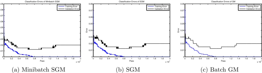
The rest of this paper is organized as follows. Section 2 introduces the learning setting and the SGM algorithm. Main results with discussions and proof sketches are presented in Section 3. Preliminary lemmas necessary for the proofs will be given in Section 4 while detailed proofs will be conducted in Sections 5 to 8. Finally, simple numerical simulations are given in Section 9 to complement our theoretical results.

Notation For anya, b∈_R,a∨b denotes the maximum ofaand b. Nis the set of all positive integers. For anyT ∈_N,[T] denotes the set{1,· · ·, T}.For any two positive sequences{at}t∈[T]

and {bt}t∈[T], the notation at . bt for all t ∈ [T] means that there exists a positive constant

C≥0 such thatC is independent oft and thatat≤Cbtfor all t∈[T].

2. Learning with SGM

We begin by introducing the learning setting we consider, and then describe the SGM learning algorithm. Following (Rosasco and Villa, 2015), the formulation we consider is close to the setting of functional regression, and covers the reproducing kernel Hilbert space (RKHS) setting as a special case, see Appendix A. In particular, it reduces to standard linear regression for finite dimensions.

2.1 Learning Problems

Let H be a separable Hilbert space, with inner product and induced norm denoted by h·,·i_H

andk · kH, respectively. Let the input space X ⊆H and the output spaceY ⊆R. Letρ be an unknown probability measure on Z =X×Y, ρX(·) the induced marginal measure on X, and

ρ(·|x) the conditional probability measure on Y with respect tox∈X and ρ.

Considering the square loss function, the problem under study is the minimization of the

risk,

inf

ω∈HE(ω), E(ω) =

Z

X×Y

(hω, xiH−y)2dρ(x, y), (1)

when the measure ρ is known only through a sample z = {zi = (xi, yi)}mi=1 of size m ∈ N,

independently and identically distributed (i.i.d.) according to ρ. In the following, we measure the quality of an approximate solution ˆω∈H (an estimator) considering the excess risk, i.e.,

E(ˆω)− inf

ω∈HE(ω). (2)

Throughout this paper, we assume that there exists a constantκ∈[1,∞[, such that

2.2 Stochastic Gradient Method

We study the following variant of SGM, possibly with mini-batches. Unlike some of the vari-ants studied in the literature, the algorithm we consider in this paper does not involve any explicit penalty term or any projection step, in which case one does not need to tune the penalty/projection parameter.

Algorithm 1 Let b ∈ [m]. Given any sample z, the b-minibatch stochastic gradient method is

defined by ω1= 0 and

ωt+1 =ωt−ηt

1 b

bt

X

i=b(t−1)+1

(hωt, xjiiH −yji)xji, t= 1, . . . , T, (4)

where {ηt>0} is a step-size sequence. Here,j1, j2,· · · , jbT are i.i.d. random variables from the

uniform distribution on [m] 1.

We add some comments on the above algorithm. First, different choices for the mini-batch sizebcan lead to different algorithms. In particular, forb= 1, the above algorithm corresponds to a simple SGM, while forb=m,it is a stochastic version of the batch gradient descent. In this paper, we are particularly interested in the cases of b = 1 and b= √m. Second, other choices on the initial value, rather than ω1 = 0, is possible. In fact, following from our proofs in this

paper, the interested readers can see that the convergence results stated in the next subsections still hold for other choices of initial values. Finally, the number of total iterations T can be bigger than the number of sample points m. This indicates that we can use the sample more than once, or in another words, we can run the algorithm with multiple passes over the data. Here and in what follows, the number of ‘passes’ over the data is referred to dbt

meattiterations

of the algorithm.

The aim of this paper is to derive excess risk bounds for Algorithm 1. Throughout this paper, we assume that {ηt}t is non-increasing, andT ∈NwithT ≥3. We denote by Jt the set

{jl:l=b(t−1) + 1,· · ·, bt} and by Jthe set{jl :l= 1,· · · , bT}.

3. Main Results with Discussions

In this section, we first state some basic assumptions. Then, we present and discuss our main results.

3.1 Assumptions

The following assumption is related to a moment assumption on |y|2_{. It is weaker than the}

often considered bounded output assumption, such as the binary classification problems where Y ={−1,1}.

Assumption 1 There exists constants M ∈]0,∞[ andv∈]1,∞[such that Z

Y

y2ldρ(y|x)≤l!Mlv, ∀l∈_N, (5)

ρX-almost surely.

To present our next assumption, we introduce the operator L_ρ : L2_{(H, ρ}

X) → L2(H, ρX),

defined byLρ(f) =

R

Xhx,·iHf(x)ρX(x). Here,L

2_{(H, ρ}

X) is the Hilbert space of square integral

functions fromH toRwith respect to ρX, with norm,

kfk_ρ=

Z

X

|f(x)|2_dρ

X(x)

1/2

.

Under Assumption (3),L_ρcan be proved to be positive trace class operators (Cucker and Zhou, 2007), and henceLζρ withζ ∈Rcan be defined by using the spectral theory.

It is well known (see e.g., Cucker and Zhou, 2007) that the function minimizing R_Z(f(x)−

y)2dρ(z) over all measurable functions f :H →_Ris the regression function, given by fρ(x) =

Z

Y

ydρ(y|x), x∈X. (6)

Define another Hilbert spaceHρ={f :X→R|∃ω ∈H with f(x) =hω, xiH, ρX-almost surely}.

Under Assumption (3), it is easy to see that Hρ is a subspace of L2(H, ρX). Let fH be the projection of the regression function fρ onto the closure of Hρ in L2(H, ρX). It is easy to see

that the search for a solution of Problem (1) is equivalent to the search of a linear function inHρ

to approximate fH. From this point of view, bounds on the excess risk of a learning algorithm onHρorH, naturally depend on the following assumption, which quantifies how well, the target

functionfH can be approximated byHρ.

Assumption 2 There exist ζ >0 and R >0, such that kL_ρ−ζfHkρ≤R.

The above assumption is fairly standard in non-parametric regression (Cucker and Zhou, 2007; Rosasco and Villa, 2015). The biggerζ is, the more stringent the assumption is, since

Lζ1

ρ(L2(H, ρX))⊆ Lζρ2(L2(H, ρX)) when ζ1 ≥ζ2.

In particular, for ζ = 0, we are making no assumption, while for ζ = 1/2, we are requiring fH∈Hρ, since (Rosasco and Villa, 2015)

Hρ=L1ρ/2(L2(H, ρX)). (7)

In the case of ζ ≥ 1/2, fH ∈ Hρ, which implies Problem (1) has at least one solution in the

spaceH. In this case, we denoteω† as the solution with the minimalH-norm. Finally, the last assumption relates to the capacity of the hypothesis space.

Assumption 3 For some γ ∈]0,1]and cγ >0, Lρ satisfies

tr(Lρ(Lρ+λI)−1)≤cγλ−γ, for all λ >0. (8)

The left hand-side of of (8) is called as the effective dimension (Caponnetto and De Vito, 2007), or the degrees of freedom (Zhang, 2005). It can be related to covering/entropy number conditions, see (Steinwart and Christmann, 2008) for further details. Assumption 3 is always true forγ = 1 andcγ =κ2, sinceLρis a trace class operator which implies the eigenvalues ofLρ, denoted asσi,

satisfy tr(Lρ) =P_iσi ≤κ2.This is referred to as the capacity independent setting. Assumption

3 with γ ∈]0,1] allows to derive better error rates. It is satisfied, e.g., if the eigenvalues ofL_ρ

3.2 Optimal Rates for SGM and Batch GM: Simplified Versions

We start with the following corollaries, which are the simplified versions of our main results stated in the next subsections.

Corollary 1 (Optimal Rate for SGM) Under Assumptions 2 and 3, let |y| ≤ M almost

surely for someM >0.Let p∗=dm

1

2ζ+γ_{eif 2ζ+γ >1, orp∗ =dm}1−_{e with∈]0,1[otherwise.} Consider the SGM with

1) b= 1, ηt' _m1 for allt∈[(p∗m)],and ω˜p∗=ωp∗m+1.

If δ ∈]0,1]and m≥mδ, then with probability2at least 1−δ, it holds

EJ[E(˜ωp∗)]−inf

H E ≤C

(

m−2ζ+γ2ζ _{when 2ζ+γ >1;}

m−2ζ(1−) otherwise. (9)

Furthermore, the above also holds for the SGM with3

2) b=√m, ηt' √1_m for allt∈[(p∗

√

m)], and ω˜p∗ =ωp∗ √

m+1.

In the above, mδ andC are positive constants depending onκ2,kTρk, M, ζ, R, cγ, γ, a polynomial

of logm and log(1/δ), and mδ also on δ (and also on kfHk∞ in the case that ζ <1/2).

We add some comments on the above result. First, the above result asserts that, at p∗ passes over the data, the SGM with two different fixed step-size and fixed mini-batch size choices, achieves optimal learning error bounds, matching (or improving) those of ridge regression (Smale and Zhou, 2007; Caponnetto and De Vito, 2007). Second, according to the above result, using mini-batch allows to use a larger step-size while achieving the same optimal error bounds. Finally, the above result can be further simplified in some special cases. For example, if we consider the capacity independent case, i.e., γ = 1, and assuming that fH ∈ Hρ, which is

equivalent to making Assumption 2 with ζ = 1/2 as mentioned before, the error bound is O(m−1/2), while the number of passes p∗ =d

√

me.

Remark 1 (Finite Dimensional Case) With a simple modification of our proofs, we can

derive similar results for the finite dimensional case, i.e.,H =Rd, where in this case,γ = 0. In

particular, lettingζ = 1/2,under the same assumptions of Corollary 1, if one considers the SGM

withb= 1 andηt' _m1 for allt∈[m2],then with high probability, EJ[E(ωm2₊₁)]−inf_HE.d/m,

provided that m&dlogd.

Remark 2 From the proofs, one can easily see that if fH and E(˜ωp∗)−infHE are replaced

respectively by f∗ ∈ L2(H, ρX) and kh·,ω˜p∗iH −f∗k

2

ρ, in both the assumptions and the error

bounds, then all theorems and their corollaries of this paper are still true, as long as f∗ satisfies

R

X(f∗ −fρ)(x)KxdρX = 0. As a result, if we assume that fρ satisfies Assumption 2 (with fH

replaced by fρ), as typically done in (Smale and Zhou, 2007; Caponnetto and De Vito, 2007;

Steinwart et al., 2009; Caponnetto and Yao, 2010) for the RKHS setting, we have that with high probability,

EJkh·,ω˜p∗iH−fρk

2

ρ≤C

(

m−

2ζ

2ζ+γ _{when2ζ+γ >1;}

m−2ζ(1−) otherwise.

In this case, the factor kfHk∞ from the upper bounds for the case ζ < 1/2 is exactly kfρk∞

and can be controlled by the condition |y| ≤M (and more generally, by Assumption 1). Since

many common RKHSs are universally consistent (Steinwart and Christmann, 2008), making

Assumption 2 onfρ is natural and moreover, deriving error bounds with respect to fρ seems to

be more interesting in this case.

As a byproduct of our proofs in this paper, we derive the following optimal results for batch gradient methods (GM), defined byν1 = 0 and

νt+1 =νt−ηt

1 m

m

X

i=1

(hνt, xiiH −yi)xi, t= 1, . . . , T. (10)

Corollary 2 (Optimal Rate for Batch GM) Under the assumptions and notations of

Corol-lary 1, consider batch GM (10) withηt'1. Ifm is large enough, then with high probability, (9)

holds for ω˜p∗ =νp∗+1.

In the above corollary, the convergence rates are optimal for 2ζ+γ >1. To the best of our knowledge, these results are the first ones with minimax rates (Caponnetto and De Vito, 2007; Blanchard and M¨ucke, 2016) for the batch GM in the non-attainable case. Particularly, they improve the results in the previous literature, see Subsection 3.6 for more discussions.

Corollaries 1 and 2 cover the main contributions of this paper. In the following subsections, we will present the main theorems of this paper, following with several corollaries and simple discussions, from which one can derive the simplified versions stated in this subsection. In the next subsection, we present results for SGM in the attainable case while results in the non-attainable case will be given in Subsection 3.4, as the bounds for these two cases are different and particularly their proofs require different estimations. At last, results with more specific convergence rates for batch GM will be presented in Subsection 3.5.

3.3 Main Results for SGM: Attainable Case

In this subsection, we present convergence results in the attainable case, i.e.,ζ ≥1/2, following with simple discussions. One of our main theorems in the attainable case is stated next, and provides error bounds for the studied algorithm. For the sake of readability, we only present results in a fixed step-size setting in this section. Results in a general setting (ηt=η1t−θ with

0≤θ <1 can be found in Section 7.

Theorem 1 Under Assumptions 1, 2 and 3, let ζ ≥ 1/2, δ ∈]0,1[, ηt = ηκ−2 for all t ∈[T],

with η ≤ _8(log1_T+1). If m ≥mδ, then the following holds with probability at least 1−δ: for all

t∈[T],

EJ[E(ωt+1)]−inf

H E ≤q1(ηt)

−2ζ_+q

2m−

2ζ

2ζ+γ_{(1 +m}−

1

2ζ+γ_ηt)2_log2_Tlog2 1

δ

+q3ηb−1(1∨m−

1

2ζ+γ_{ηt) logT.}

(11)

Here,mδ, q1, q2 andq3 are positive constants depending onκ2,kTρk, M, v, ζ, R, cγ, γ, andmδalso

onδ (which will be given explicitly in the proof ).

Solving this trade-off problem leads to different choices onη,T, andb, corresponding to different regularization strategies, as shown in subsequent corollaries.

The first corollary gives generalization error bounds for simple SGM, with a universal step-size depending on the number of sample points.

Corollary 3 Under Assumptions 1, 2 and 3, let ζ ≥ 1/2 , δ ∈]0,1[, b= 1 and ηt ' _m1 for all

t∈[m2]. Ifm≥mδ,then with probability at least 1−δ, there holds

EJ[E(ωt+1)]−inf

H E .

m

t

2ζ

+m−2ζ+22ζ+γ

t

m

2

·log2mlog2 1

δ, ∀t∈[m

2_{], (12)}

and in particular,

EJ[E(ωT∗₊₁)]−inf

H E .m

−_2ζ+γ2ζ

log2mlog21

δ, (13)

where T∗ =dm

2ζ+γ+1

2ζ+γ e_{.Here, m}

δ is exactly the same as in Theorem 1.

Remark 3 Ignoring the logarithmic term and letting t=pm, Eq. (12) becomes

EJ[E(ωpm+1)]−inf

H E.p

−2ζ_+m−2ζ+2

2ζ+γ_p2_.

A smaller p may lead to a larger bias, while a largerp may lead to a larger sample error. From

this point of view, p has a regularization effect.

The second corollary provides error bounds for SGM with a fixed mini-batch size and a fixed step-size (which depend on the number of sample points).

Corollary 4 Under Assumptions 1, 2 and 3, letζ ≥1/2, δ∈]0,1[,b=d√meand ηt' √1_m for

allt∈[m2]. If m≥mδ,then with probability at least 1−δ, there holds

EJ[E(ωt+1)]−inf

H E.

√

m t

2ζ

+m−

2ζ+2 2ζ+γ

t

√

m

2

log2mlog2 1

δ, ∀t∈[m

2_{], (14)}

and particularly,

EJ[E(ωT∗₊₁)]−inf

H E .m

−_2ζ+γ2ζ

log2mlog21

δ, (15)

where T∗ =dm2ζ+γ1 +

1

2_e.

The above two corollaries follow from Theorem 1 with the simple observation that the dominating terms in (11) are the terms related to the bias and the sample variance, when a small step-size is chosen. The only free parameter in (12) and (14) is the number of iterations/passes. The ideal stopping rule is achieved by balancing the two terms related to the bias and the sample variance, showing the regularization effect of the number of passes. Since the ideal stopping rule depends on the unknown parametersζ and γ, a hold-out cross-validation procedure is often used to tune the stopping rule in practice. Using an argument similar to that in Chapter 6 from (Steinwart and Christmann, 2008), it is possible to show that this procedure can achieve the same convergence rate.

We give some further remarks. First, the upper bound in (13) is optimal up to a logarithmic factor, in the sense that it matches the minimax lower rate in (Caponnetto and De Vito, 2007;

over the data are needed to obtain optimal rates in both cases. Finally, in comparing the simple SGM and the mini-batch SGM, Corollaries 3 and 4 show that a larger step-size is allowed to use for the latter.

In the next result, both the step-size and the stopping rule are tuned to obtain optimal rates for simple SGM with multiple passes. In this case, the step-size and the number of iterations are the regularization parameters.

Corollary 5 Under Assumptions 1, 2 and 3, letζ ≥1/2, δ ∈]0,1[, b= 1 and ηt'm

− 2ζ

2ζ+γ _for

allt∈[m2]. If m≥mδ, and T∗ =dm

2ζ+1

2ζ+γ_{e,then (13) holds with probability at least1−δ.}

The next corollary shows that for some suitable mini-batch sizes, optimal rates can be achieved with a constant step-size (which is nearly independent of the number of sample points) by early stopping.

Corollary 6 Under Assumptions 1, 2 and 3, let ζ ≥1/2, δ∈]0,1[, b=dm

2ζ

2ζ+γ_{e andη}

t' _log1_m

for allt∈[m]. If m≥mδ,and T∗=dm

1

2ζ+γ_{e,then (13) holds with probability at least 1−δ.}

According to Corollaries 5 and 6, aroundm

1−γ

2ζ+γ _{passes over the data are needed to achieve}

the best performance in the above two strategies. In comparisons with Corollaries 3 and 4

where aroundm

ζ+1

2ζ+γ _{passes are required, the latter seems to require fewer passes over the data.}

However, in this case, one might have to run the algorithms multiple times to tune the step-size, or the mini-batch size.

Remark 4 1) If we make no assumption on the capacity, i.e.,γ = 1, Corollary 5 recovers the result in (Ying and Pontil, 2008) for one pass SGM.

2) If we make no assumption on the capacity and assume thatfH∈Hρ, from Corollaries 5 and

6, we see that the optimal convergence rate O(m−1/2) can be achieved after one pass over the

data in both of these two strategies. In this special case, Corollaries 5 and 6 recover the results for one pass SGM in, e.g., (Shamir and Zhang, 2013; Dekel et al., 2012).

The next result gives generalization error bounds for ‘batch’ SGM with a constant step-size (nearly independent of the number of sample points).

Corollary 7 Under Assumptions 1, 2 and 3, let ζ ≥ 1/2, δ ∈]0,1[, b = m and ηt ' _log1_m for

allt∈[m]. If m≥mδ, andT∗ =dm

1

2ζ+γe_{, then (13) holds with probability at least1}−_δ.

Theorem 1 and its corollaries give convergence results with respect to the target function values. In the next theorem and corollary, we will present convergence results inH-norm.

Theorem 2 Under the assumptions of Theorem 1, the following holds with probability at least

1−δ: for allt∈[T]

EJ[kωt−ω†k2H]≤q1(ηt)1−2ζ+q2m−

2ζ−1

2ζ+γ_{(1 +m}−

1

2ζ+γ_ηt)2_log2_Tlog2 1

δ +q3η

2_tb−1_{. (16)}

Here,q1, q2 andq3 are positive constants depending on κ2,kTρk, M, v, ζ, R, cγ, and γ (which can

The proof of the above theorem is similar as that for Theorem 1, and will be given in Subsection 8. Again, the upper bound in (16) is composed of three terms related to bias, sample variance, and computational variance. Balancing these three terms leads to different choices onη,T, and b, as shown in the following corollary.

Corollary 8 With the same assumptions and notations from any one of Corollaries 3 to 7, the

following holds with probability at least 1−δ:

EJ[kωT∗₊₁−ω†k2_H].m−

2ζ−1

2ζ+γ_log2_mlog21

δ.

The convergence rate in the above corollary is optimal up to a logarithmic factor, as it matches the minimax rate shown in (Blanchard and M¨ucke, 2016).

In the next subsection, we will present convergence results in the non-attainable case, i.e., ζ <1/2.

3.4 Main Results for SGM: Non-attainable Case

Our main theorem in the non-attainable case is stated next, and provides error bounds for the studied algorithm. Here, we present results with a fixed step-size, whereas general results with a decaying step-size will be given in Section 7.

Theorem 3 Under Assumptions 1, 2 and 3, let ζ ≤ 1/2, δ ∈]0,1[, ηt = ηκ−2 for all t ∈ [T],

with 0 < η ≤ 1

8(logT+1). Then the following holds for all t∈[T] with probability at least 1−δ:

1) if 2ζ+γ >1 andm≥mδ,then

EJ[E(ωt+1)]−inf

H E ≤

q1(ηt)−2ζ+q2m−

2ζ 2ζ+γ

(1∨m−2ζ+γ1 _ηt)3_log4_Tlog21

δ

+q3ηb−1(1∨m

− 1

2ζ+γ_{ηt) logT;}

(17)

2) if 2ζ+γ ≤1 and for some∈]0,1[, m≥mδ,, then

EJ[E(ωt+1)]−inf

H E ≤

q1(ηt)−2ζ+q2mγ(1−)−1

(1∨ηm−1t)3log4Tlog2 1 δ +q3ηb−1(1∨m−1ηt) logT.

Here,mδ(ormδ,),q1, q2andq3 are positive constants depending only onκ2,kTρk, M, v, ζ, R, cγ, γ,

kfHk∞, and mδ (or mδ,) also onδ (and ).

The upper bounds in (11) (for the attainable case) and (17) (for the non-attainable case) are similar, whereas the latter has an extra logarithmic factor. Consequently, in the subsequent

corollaries, we deriveO(m−

2ζ

2ζ+γ_log4_{m) for the non-attainable case. In comparison with that for}

the attainable case, the convergence rate for the non-attainable case has an extra log2mfactor. Similar to Corollaries 3 and 4, and as direct consequences of the above theorem, we have the following generalization error bounds for the studied algorithm with different choices of parameters in the non-attainable case.

Corollary 9 Under Assumptions 1, 2 and 3, let ζ ≤ 1/2 , δ ∈]0,1[, b= 1 and ηt ' _m1 for all

t∈[m2]. With probability at least 1−δ, the following holds:

1) if 2ζ+γ >1, m≥mδ and T∗ =dm

1+2ζ+γ

2ζ+γ _{e, then}

EJ[E(ωT∗₊₁)]−inf

H E .m

− 2ζ

2ζ+γ_log4_mlog21

2) if2ζ+γ ≤1, and for some ∈]0,1[, m≥mδ,, and T∗ =dm2−e, then

EJ[E(ωT∗₊₁)]−inf

H E.m

−2ζ(1−)_log4_mlog2 1

δ. (19)

Here, mδ and mδ, are given by Theorem 3.

Corollary 10 Under Assumptions 1, 2 and 3, let ζ ≤1/2, δ∈]0,1[, b'√m andηt' √1_m for

allt∈[m2]. With probability at least 1−δ, there holds

1) if2ζ+γ >1, m≥mδ and T∗ =dm

1

2ζ+γ+

1

2e_{, then (18) holds;}

2) if2ζ+γ ≤1, for some ∈]0,1[, m≥mδ,, and T∗=dm

3

2−e, then (19) holds.

The convergence rates in the above corollaries, i.e., m−

2ζ

2ζ+γ _{if 2ζ +γ > 1 or m}−2ζ(1−)

otherwise, match those in (Dieuleveut and Bach, 2016) for one pass SGM with averaging, up to a logarithmic factor. Also, in the capacity independent case, i.e.,γ = 1, the convergence rates

in the above corollary read asm−

2ζ

2ζ+1 _{(since 2ζ+γ is always bigger than 1), which are exactly}

the same as those in (Ying and Pontil, 2008) for one pass SGM.

Similar results to Corollaries 5–7 can be also derived for the non-attainable case by applying Theorem 3. Refer to Appendix B for more details.

3.5 Main Results for Batch GM

In this subsection, we present convergence results for batch GM. As a byproduct of our proofs in this paper, we have the following convergence rates for batch GM.

Theorem 4 Under Assumptions 1, 2 and 3, set ηt ' 1, for all t ∈ [m]. Let T∗ = dm

1

2ζ+γe

if 2ζ +γ > 1, or T∗ = dm1−e with ∈]0,1[ otherwise. Then with probability at least 1−δ

(0< δ <1), the following holds for the learning sequence generated by (10):

1) ifζ >1/2 and m≥mδ, then

E(νT∗+1)−inf

H E.m

− 2ζ

2ζ+γ _log2_mlog2 1

δ;

2) ifζ ≤1/2,2ζ+γ >1 and m≥mδ, then

E(νT∗+1)−inf

H E.m

−_2ζ+γ2ζ

log4mlog2 1 δ;

3) if2ζ+γ ≤1 and m≥mδ,, then

E(νT∗+1)−inf

H E .m

−2ζ(1−)_log4_mlog2 1

δ.

Here, mδ (or mδ,), and all the constants in the upper bounds are positive and depend only on

κ2,kT_ρk, M, v, ζ, R, cγ, γ, kfHk∞, and mδ (or mδ,) also onδ (and ).

3.6 Discussions

capacity independent rate of order O(m−

2ζ

2ζ+1_{logm) with a fixed step-size η} ' _m− 2ζ 2ζ+1_{, and}

Dieuleveut and Bach (2016) derived capacity dependent error bounds of order O(m−

2 min(ζ,1)

2 min(ζ,1)+γ₎

(when 2ζ+γ >1) for the average. Note also that a regularized version of SGM has been studied

in (Tarres and Yao, 2014), where the derived convergence rate is of order O(m−

2ζ

2ζ+1_{) assuming}

that ζ ∈ [1₂,1]. In comparison with these existing convergence rates, our rates from (13) are comparable, either involving the capacity condition, or allowing a broader regularity parameter ζ (which thus improves the rates). For finite dimensional cases, it has been shown in (Bach and Moulines, 2013) that one pass SGM with averaging with a constant step-size achieves the optimal convergence rate of O(d/m). In comparisons, our results for multi-pass SGM with a smaller step-size seems to be suboptimal in the computational complexity, as we needmpasses over the data to achieve the same rate. The reason for this may arise from “the computational error” that will be introduced later, or the fact that we do not consider an averaging step as done in (Bach and Moulines, 2013). We hope that in the future by considering a larger step-size and averaging, one can reduce the computational complexity of multi-pass SGM while achieving the same rate.

More recently, Rosasco and Villa (2015) studied multiple passes SGM with a fixed ordering at each pass, also called incremental gradient method. Making no assumption on the capacity, rates of orderO(m−ζ+1ζ _{) (inL}2_{(H, ρ}

X)-norm) with a universal step-sizeη'1/mare derived. In

comparisons, Corollary 3 achieves better rates, while considering the capacity assumption. Note also that Rosasco and Villa (2015) proved sharp rate in H-norm for ζ ≥ 1/2 in the capacity independent case. In comparisons, we derive optimal capacity-dependent rate, considering mini-batches.

The idea of using mini-batches (and parallel implements) to speed up SGM in a general stochastic optimization setting can be found, e.g., in (Shalev-Shwartz et al., 2011; Dekel et al., 2012; Sra et al., 2012; Ng, 2016). Our theoretical findings, especially the interplay between the mini-batch size and the step-size, can give further insights on parallelization learning. Besides, it has been shown in (Cotter et al., 2011; Dekel et al., 2012) that for one pass mini-batch SGM with a fixed step-sizeη 'b/√m and a smooth loss function, assuming the existence of at least one solution in the hypothesis space for the expected risk minimization, the convergence rate is of order O(p1/m+b/m) by considering an averaging scheme. When adapting to the learning setting we consider, this reads as that if fH ∈ Hρ, i.e., ζ = 1/2, the convergence rate for the

average isO(p1/m+b/m). Note that,fH does not necessarily belong to Hρ in general. Also,

our derived convergence rate from Corollary 4 is better, when the regularity parameter ζ is greater than 1/2,orγ is smaller than 1.

For batch GM in the attainable case, convergent results with optimal rates have been derived in, e.g, (Bauer et al., 2007; Caponnetto and Yao, 2010; Blanchard and M¨ucke, 2016; Dicker et al.,

2017). In particular, Bauer et al. (2007) proved convergence ratesO(m−

2ζ

2ζ+1_{) without}

consider-ing Assumption 3, and Caponnetto and Yao (2010) derived convergence rates O(m−2ζ+γ2ζ _).For

the non-attainable case, convergent results with suboptimal rates O(m −2ζ

2ζ+2_{) can be found in}

(Yao et al., 2007), and to the best of our knowledge, the only result with optimal rateO(m −2ζ

2ζ+γ₎

We end this discussion with some further comments on batch GM and simple SGM. First, according to Corollaries 1 and 2, it seems that both simple SGM (with step-sizeηt'm−1) and

batch GM (with step-sizeηt'1) have the same computational complexities (which are related

to the number of passes) and the same orders of upper bounds. However, there is a subtle difference between these two algorithms. As we see from (22) in the coming subsection, every m iterations of simple SGM (with step-size ηt ' m−1) corresponds to one iteration of batch

GM (with step-size ηt'1). In this sense, SGM discretizes and refines the regularization path

of batch GM, which thus may lead to smaller generalization errors. This phenomenon can be further understood by comparing our derived bounds, (11) and (73), for these two algorithms. Indeed, if one can ignore the computational error, one can easily show that the minimization (overt) of right hand-side of (11) with η'm−1 is always smaller than that of (73) with η'1. At last, by Corollary 6, using a larger step-size for SGM allows one to stop earlier (while sharing the same optimal rates), which thus reduces the computational complexity. This suggests that SGM may have some computational advantage over batch GM.

3.7 Proof Sketch (Error Decomposition)

The key to our proof is a novel error decomposition, which may be also used in analysing other learning algorithms. One may also use the approach in (Bousquet and Bottou, 2008; Lin et al., 2016b,a) which is based on the following error decomposition,

EE(ωt)−inf

H E = [E(E(ωt)− Ez(ωt)) +EEz(˜ω)− E(˜ω)] +E(Ez(ωt)− Ez(˜ω)) +E(˜ω)−infH E,

where ˜ω ∈ H is some suitably intermediate element and Ez denotes the empirical risk over z,

i.e.,

E_z(·) = 1 m

m

X

i=1

(h·, xii −yi)2. (20)

However, one can only derive a sub-optimal convergence rate, since the proof procedure involves upper bounding the learning sequence to estimate the sample error (the first term of right-hand side). Also, in this case, the ‘regularity’ of the regression function can not be fully utilized for estimating the bias (the last term). Thanks to the property of squares loss, we can exploit a different error decomposition leading to better results.

To describe the decomposition, we need to introduce two sequences. Thepopulation iteration

is defined byµ1 = 0 and

µt+1=µt−ηt

Z

X

(hµt, xiH −fρ(x))xdρX(x), t= 1, . . . , T. (21)

The above iterated procedure is ideal and can not be implemented in practice, since the distri-bution ρX is unknown in general. Replacing ρX by the empirical measure andfρ(xi) by yi, we

derive thesample iteration (associated with the samplez), i.e., (10). Clearly,µtis deterministic

and νt is a H-valued random variable depending on z. Given the samplez, the sequence {νt}t

has a natural relationship with the learning sequence{ωt}t, since

EJ[ωt] =νt. (22)

Indeed, taking the expectation with respect toJton both sides of (4), and noting thatωtdepends

only onJ1,· · · ,Jt−1 (given anyz), one has

EJt[ωt+1] =ωt−ηt

1 m

m

X

i=1

and thus,

EJ[ωt+1] =EJ[ωt]−ηt

1 m

m

X

i=1

(h_EJ[ωt], xiiH−yi)xi, t= 1, . . . , T,

which satisfies the iterative relationship given in (10). By an induction argument, (22) can then be proved.

Let Sρ :H → L2(H, ρX) be the linear map defined by (Sρω)(x) = hω, xiH,∀ω, x ∈ H. We

have the following error decomposition.

Proposition 1 We have

EJ[E(ωt)]−inf

H E ≤2kSρµt−fHk

2

ρ+ 2kSρνt− Sρµtk2ρ+EJ[kSρωt− Sρνtk2ρ]. (23)

Proof For any ω∈H, we have (Rosasco and Villa, 2015)

E(ω)− inf

ω∈HE(ω) =kSρω−fHk

2

ρ.

Thus,E(ωt)−infHE =kSρωt−fHk2ρ,and

EJ[kSρωt−fHk2ρ] =EJ[kSρωt− Sρνt+Sρνt−fHk2ρ]

=EJ[kSρωt− Sρνtk2ρ+kSρνt−fHk2ρ] + 2EJhSρωt− Sρνt,Sρνt−fHiρ.

Using (22) in the above equality, we get,

EJ[kSρωt−fHk2ρ] =EJ[kSρωt− Sρνtk2ρ+kSρνt−fHk2ρ].

The proof is finished by considering,

kSρνt−fHk2_ρ=kSρνt− Sρµt+Sρµt−fHk2_ρ≤2kSρνt− Sρµtkρ2+ 2kSρµt− SρfHk2_ρ.

There are three terms in the upper bound of the error decomposition (23). We refer to the deterministic term kSρµt−fHk2ρ as the bias, the term kSρνt− Sρµtk2ρ depending on z as the

sample variance, and EJ[kSρωt− Sρνtk2ρ] as the computational variance. The bias term, which

is deterministic, has been well studied in the literature, see e.g., (Yao et al., 2007) and also (Rosasco and Villa, 2015). The main novelties of this paper are the estimate of the sample and computational variances and the difficult part is the estimate of the computational variances. The proof of these results is quite lengthy and makes use of some ideas from (Yao et al., 2007; Smale and Zhou, 2007; Bauer et al., 2007; Ying and Pontil, 2008; Tarres and Yao, 2014; Rudi et al., 2015). These three error terms will be estimated in Sections 5 and 6. The bounds in Theorems 1 and 3 thus follow plugging these estimations in the error decomposition, see Section 7 for more details. The proof for Theorem 2 is similar, see Section 8 for the details.

4. Preliminary Analysis

4.1 Notation

We first introduce some notations. For t ∈ N, ΠTt+1(L) =

QT

k=t+1(I −ηkL) for t ∈ [T −1]

and ΠT_T+1(L) = I, for any operator L : H → H, where H is a Hilbert space and I de-notes the identity operator on H. E[ξ] denotes the expectation of a random variable ξ. For a given bounded operator L : L2(H, ρX) → H, kLk denotes the operator norm of L, i.e.,

kLk = sup_f∈L2_(H,ρ

X),kfkρ=1kLfkH. We will use the conventional notations on summation and

production: Qt

i=t+1 = 1 and

Pt

i=t+1= 0.

We next introduce some auxiliary operators. Let Sρ : H → L2(H, ρX) be the linear map

ω → hω,·i_H, which is bounded by κ under Assumption (3). Furthermore, we consider the adjoint operatorS_ρ∗ :L2(H, ρX)→H, the covariance operatorTρ:H→H given byTρ=Sρ∗Sρ,

and the operator Lρ : L2(H, ρX) → L2(H, ρX) given by SρSρ∗. It can be easily proved that

S∗

ρg=

R

Xxg(x)dρX(x) and Tρ=

R

Xh·, xiHxdρX(x).The operatorsTρ and Lρ can be proved to

be positive trace class operators (and hence compact). For any ω ∈ H, it is easy to prove the following isometry property (Steinwart and Christmann, 2008)

kS_ρωk_ρ=kp

T_ρωk_H. (24)

We define the sampling operatorS_x :H →_Rm _{by (S}

xω)i =hω, xiiH, i∈[m], where the norm

k · k_Rm in_Rm is the Euclidean norm times 1/

√

m. Its adjoint operator S_x∗ :Rm → H, defined by hS_x∗y, ωi_H =hy,SxωiRm fory∈Rm is thus given by S

∗

xy= m1

Pm

i=1yixi.Moreover, we can

define the empirical covariance operatorT_x:H →H such thatT_x=S∗

xSx. Obviously,

Tx=

1 m

m

X

i=1

h·, xiiHxi.

With these notations, (21) and (10) can be rewritten as

µt+1=µt−ηt(Tρµt− Sρ∗fρ), t= 1, . . . , T, (25)

and

νt+1 =νt−ηt(Txνt− Sx∗y), t= 1, . . . , T, (26)

respectively.

Using the projection theorem, one can prove that

S_ρ∗fρ=Sρ∗fH. (27)

Indeed, since fH is the projection of the regression function fρ onto the closure of Hρ in

L2(H, ρX),according to the projection theorem, one has

hfH−fρ,Sρωiρ= 0, ∀ω∈H,

which can be written as

hS_ρ∗fH− Sρ∗fρ, ωiH = 0, ∀ω∈H,

4.2 Concentration Inequality

We need the following concentration result for Hilbert space valued random variable used in (Caponnetto and De Vito, 2007) and based on the results in (Pinelis and Sakhanenko, 1986).

Lemma 11 Letw1,· · · , wmbe i.i.d random variables in a Hilbert space with normk·k. Suppose

that there are two positive constantsB andσ2 such that

E[kw1−E[w1]kl]≤

1 2l!B

l−2_σ2_{, ∀l≥2. (28)}

Then for any 0< δ <1, the following holds with probability at least 1−δ,

1 m

m

X

k=1

wm−E[w1]

≤2

B

m +

σ

√

m

log2 δ.

In particular, (28) holds if

kw1k ≤B/2 a.s., and E[kw1k2]≤σ2. (29) 4.3 Basic Estimates

Finally, we introduce the following three basic estimates, whose proofs can be found in Appendix C.

Lemma 12 Let θ∈[0,1[, and t∈_N. Then

t1−θ

2 ≤

t

X

k=1

k−θ ≤ t 1−θ

1−θ.

Lemma 13 Let θ∈_R and t∈_N. Then

t

X

k=1

k−θ≤tmax(1−θ,0)(1 + logt).

Lemma 14 Let q∈_R andt∈_N witht≥3. Then

t−1

X

k=1

1 t−kk

−q _≤2t−min(q,1)_{(1 + logt).}

In the next sections, we begin prooving the main results. The proofs are quite lengthy and they are divided into several steps. For the ease of readability, we list some of the notations and definitions in Appendix D. We also remark that we are particularly interested in developing error bounds in terms of the stepsizeηt(=η1t−θ), the number of iterationstorT, the ‘regularization’

parameterλ >0, the sample sizem, the minibatch sizeb, and the failing profitability δ. Other parameters such as κ2,kT_ρk, M, v, R, cγ and kfHk∞ can be always viewed as some constants, which are less important in our error bounds.

5. Estimating Bias and Sample Variance

5.1 Bias

In this subsection, we develop upper bounds for the bias, i.e.,kS_ρµt−fHk2ρ. Towards this end,

we introduce the following lemma, whose proof borrows idea from (Ying and Pontil, 2008; Tarres and Yao, 2014).

Lemma 15 Let L be a compact, positive operator on a separable Hilbert spaceH. Assume that

η1kLk ≤1. Then for t∈Nand any non-negative integer k≤t−1,

kΠt_k+1(L)Lζk ≤ ζ

ePt

j=k+1ηj

!ζ

. (30)

Proof Let{σi} be the sequence of eigenvalues ofL.We have

kΠt_k+1(L)Lζk= sup

i t

Y

l=k+1

(1−ηlσi)σζ_i.

Using the basic inequality

1 +x≤ex for all x≥ −1, (31)

withηlkLk ≤1, we get

kΠt_k+1(L)Lζk ≤ sup

i

exp

(

−σi t

X

l=k+1

ηl

)

σ_iζ

≤ sup

x≥0

exp

(

−x

t

X

l=k+1

ηl

)

xζ.

The maximum of the functiong(x) = e−cxxζ( with c > 0) over R+ is achieved at xmax= ζ/c,

and thus

sup

x≥0

e−cxxζ=

ζ ec

ζ

. (32)

Using this inequality, one can get the desired result (30).

With the above lemma and Lemma 12, we can derive the following result for the bias.

Proposition 2 Under Assumption 2, let η1κ2≤1. Then, for any t∈N,

kS_ρµt+1−fHkρ≤R

ζ 2Pt

j=1ηj

!ζ

. (33)

In particular, if ηt=ηt−θ for all t∈N, withη∈]0, κ−2]and θ∈[0,1[,then

kSρµt+1−fHkρ≤Rζζη−ζt(θ−1)ζ. (34)

Lemma 16 Under Assumption 2, let η1κ2≤1. The following holds for allt∈N:

1) If ζ ≥1/2,

kµt+1kH ≤Rκ2ζ−1. (35)

2) If ζ ∈]0,1/2],

kµt+1kH ≤R







κ2ζ−1∨

t

X

k=1

ηk

!1₂−ζ





. (36)

Proof The proof can be found in Appendix C. The proof for a fixed step-size (i.e.,ηt=ηfor all

t) can be also found in (Rosasco and Villa, 2015). For a general step-size, the proof is similar. Note also that our proof for the non-attainable case is simpler than that in (Rosasco and Villa, 2015).

5.2 Sample Variance

In this subsection, we estimate the sample variance, i.e., E[kSρµt− Sρνtk2ρ].Towards this end,

we need some preliminary analysis. We first introduce the following key inequality, which also provides the basic idea on estimatingE[kSρµt− Sρνtk2ρ].

Lemma 17 For all t∈[T],we have

kSρνt+1− Sρµt+1kρ≤ t

X

k=1

ηk

T

1 2

ρ Πtk+1(Tx)Nk

H

, (37)

where

Nk= (Tρµk− Sρ∗fρ)−(Txµk− Sx∗y), ∀k∈[T]. (38)

Proof Since νt+1 and µt+1 are given by (26) and (25), respectively,

νt+1−µt+1 = νt−µt+ηt

(Tρµt− Sρ∗fρ)−(Txνt− Sx∗y)

= (I−ηtTx)(νt−µt) +ηt

(Tρµt− Sρ∗fρ)−(Txµt− Sx∗y) ,

which is exactly

νt+1−µt+1= (I−ηtTx)(νt−µt) +ηtNt.

Applying this relationship iteratively, withν1 =µ1 = 0,

νt+1−µt+1 = Πt1(Tx)(ν1−µ1) +

t

X

k=1

ηkΠtk+1(Tx)Nk= t

X

k=1

ηkΠtk+1(Tx)Nk. (39)

By (24), we have

kS_ρνt+1− Sρµt+1kρ=

t

X

k=1

ηkT

1 2

ρ Πtk+1(Tx)Nk

H

,

which leads to the desired result (37).

bound

T

1 2

ρ Πt_k+1(Tx)Nk

H

.A detailed look at this latter term indicates that one may analyze the

termsT

1 2

ρ Πt_k+1(Tx) and Nk separately, sinceEz[Nk] = 0 and the properties of the deterministic

sequence {µk}k have been derived in Section 5.1. Moreover, to exploit the capacity condition

from Assumption 3, we estimatek(Tρ+λ)−

1

2N_kk_H (with λ > 0 properly chosen later), rather

thankNkkH, as follows.

Lemma 18 Under Assumptions 1, 2 and 3, let {Nt}t be as in (38). Then for any fixed λ >0,

andT ≥2,

1) ifζ ≥1/2,with probability at least 1−δ1, the following holds for all k∈N:

k(Tρ+λ)−

1

2N_kk_H ≤4(Rκ2ζ+

√

M) κ

m√λ+

p

2√vcγ

√

mλγ

!

log 4 δ1

. (40)

2) ifζ ∈]0,1/2[, with probability at least 1−δ1, the following holds for all k∈[T] :

k(Tρ+λ)−

1

2N_kk_H ≤2

3kfHk∞+ 2

√

M+κR

κ

m√λ+

p

2√vcγ

√

mλγ

!

log3T δ1

+

2κ2RPk i=1ηi

1₂−ζ

m√λ log

3T δ1

+√2κR

mλ 1

Pk

i=1ηi

!ζ

log3T δ1

. (41)

Proof We will apply Bernstein inequality from Lemma 11 to prove the result.

Attainable Case: ζ ≥1/2. See Appendix C for the proof.

Non-attainable case: 0< ζ <1/2.

Let wi = (fH(xi) −yi)(Tρ +λ)−1/2xi, for all i ∈ [m]. Noting that by (27), and taking the

expectation with respect to the random variable (x, y) (from the distribution ρ),

E[ω] =E[(fH(x)−fρ(x))(Tρ+λ)−1/2x] = 0.

Applying H¨older’s inequality, for anyl≥2,

E[kw−E[w]klH] =E[kwklH]≤2l−1E[(|fH(x)|l+|y|l)k(Tρ+λ)−1/2xklH]

≤2l−1

Z

X

(kfHkl∞+

Z

Y

|y|l_dρ(y|x))k(T

ρ+λ)−1/2xklHdρX(x).

Using Cauchy-Schwarz’s inequality and Assumption 1 which implies,

Z

Y

yldρ(y|x)≤

Z

Y

|y|2ldρ(y|x)

1

2

≤ √

l!Ml_v≤l!(√_M)l√_{v, (42)}

we get

E[kw−E[w]klH]≤2l−1(kfHkl∞+l!(

√

M)l√v)

Z

X

k(T_ρ+λ)−1/2xkl_HdρX(x). (43)

By Assumption (3),

k(Tρ+λI)−

1

2xk_H ≤ k√xkH

λ ≤

κ

√

Besides, using the fact that E[kξk2H] =E[tr(ξ⊗ξ)] = tr(E[ξ⊗ξ]) and E[x⊗x] =Tρ, we know

that

Z

X

k(Tρ+λI)−

1

2xk2

HdρX(x) = tr((Tρ+λI)−

1

2T_ρ(T_ρ+λI)−

1

2) = tr((T_ρ+λI)−1T_ρ),

and as a result of the above and Assumption 3,

Z

X

k(T_ρ+λI)−12xk2

HdρX(x)≤cγλ−γ.

It thus follows that

Z

X

k(T_ρ+λ)−1/2xkl

HdρX(x)≤

κ

√

λ

l−2Z

X

k(T_ρ+λ)−1/2xk2

HdρX(x)≤

κ

√

λ

l−2

cγλ−γ. (45)

Plugging the above inequality into (43),

E[kw−E[w]klH] ≤ 2l−1(kfHkl∞+l!(

√

M)l√v)

κ

√

λ

l−2

cγλ−γ

≤ 1

2l!

2κ(kfHk∞+

√

M)

√

λ

!l−2

4cγ

√

v(kfHk∞+

√

M)2λ−γ.

Therefore, using Lemma 11, we get that with probability at least 1−δ,

(T_ρ+λ)−12 1

m

m

X

i=1

(fH(xi)−yi)xi

H = 1 m m X i=1

(E[wi]−wi)

H ≤4( √

M +kfHk∞) κ m√λ+

p√ vcγ √ mλγ ! log2

δ. (46)

We next let ξi= (Tρ+λ)−1/2(hµk, xii −fH(xi))xi,for all i∈[m]. We assume thatk≥2. (The

proof for the case k= 1 is simpler as µ1 = 0.) It is easy to see that the expectation of each ξi

with respect to the random variable (xi, yi) is

E[ξ] = (Tρ+λ)−1/2(Tρµk− Sρ∗fH) = (Tρ+λ)−1/2(Tρµk− Sρ∗fρ),

and

kξkH ≤(kSρµkk∞+kfHk∞)k(Tρ+λ)−1/2xkH.

By Assumption (3),kS_ρµkk∞≤κkµkkH. It thus follows from the above and (44) that

kξkH ≤(κkµkkH+kfHk∞) κ

√

λ.

Besides,

Ekξk2H ≤

κ2

λE(µk(x)−fH(x))

2 ₌ κ2

λkSρµk−fHk

2

ρ≤

κ2R2 λ

ζ

2Pk−1

i=1 ηi

!2ζ

≤ κ 2_R2

λ

1

Pk

i=1ηi

!2ζ

where for the last inequality, we used (33). Applying Lemma 11 and (36), we get that with probability at least 1−δ,

(T_ρ+λ)−1/2[1 m

m

X

i=1

(µk(xi)−fH(xi))xi−(Tρµk− Sρ∗fρ)]

H

≤ 2κ





κkµkkH+kfHk∞

m√λ +

R

√

mλ

1

Pk

i=1ηi

!ζ

log

2 δ

≤ 2κ



 

κR+kfHk∞

m√λ +

κR

Pk

i=1ηi

1₂−ζ

m√λ +

R

√

mλ

1

Pk

i=1ηi

!ζ   log 2 δ.

Introducing the above estimate and (46) into the following inequality

k(T_ρ+λ)−1/2NkkH ≤

(T_ρ+λ)−12 1

m

m

X

i=1

(fH(xi)−yi)xi

H +

(T_ρ+λ)−1/2[1 m

m

X

i=1

(µk(xi)−fH(xi))xi−(Tρµk− Sρ∗fρ)]

H ,

and then substituting with (36), by a simple calculation, one can prove the desired result by scalingδ.

The next lemma is from Rudi et al. (2015), and is derived applying a recent Bernstein inequality from (Tropp, 2012; Minsker, 2011) for a sum of random operators.

Lemma 19 Let δ2∈(0,1)and 9κ

2

m log m

δ2 ≤λ≤ kTρk.Then the following holds with probability

at least1−δ2,

k(Tx+λI)−

1

2T

1 2

ρ k ≤ k(Tx+λI)−

1

2(T_ρ+λI)

1

2k ≤2. (47)

Now we are in a position to estimate the sample variance.

Proposition 3 Under Assumptions 1, 2 and 3, let η1κ2 ≤1 and 0 < λ≤ kTρk. Assume that

(47) holds. Then for allt∈[T] :

1) ifζ ≥1/2,and (40) hold, then for t∈N,

kS_ρνt+1− Sρµt+1kρ

≤4(Rκ2ζ+√M) κ m√λ+

p

2√vcγ

√

mλγ

! _t−1

X

k=1

2ηk

Pt

i=k+1ηi

+ 4λ

t−1

X

k=1

ηk+

√

2κ2ηt

!

log 4 δ1

2) if ζ <1/2,and (41) hold for anyt∈[T], then for t∈[T] :

kSρνt+1− Sρµt+1kρ≤ t−1

X

k=1

2ηk

Pt

i=k+1ηi

+ 4λ

t−1

X

k=1

ηk+

√

2κ2ηt

!

×



2

3kfHk∞+ 3

√

M +κR κ

m√λ+

p

2√vcγ

√

mλγ

!

+ 2κ

2_R Pt

i=1ηi

1₂−ζ

m√λ



log

3T δ1

+√2κR

mλlog 3T δ1   

t−1

X

k=1

2ηk

Pk

i=1ηi

ζ

Pt

i=k+1ηi

+ 4λ

t−1

X

k=1

ηk

Pk

i=1ηi

ζ +

√

2κ2ηt

Pt

i=1ηi

ζ





. (49)

Proof For notational simplicity, we letTρ,λ =Tρ+λI andTx,λ=Tx+λI.Note that by Lemma

17, we have (37). When k∈[t−1], by rewriting T

1 2

ρ Πt_k+1(Tx)Nk as

T 1 2 ρ T −1 2

x,λ T

1 2

x,λΠ t

k+1(Tx)T

1 2

x,λT

−1 2

x,λT

1 2

ρ,λT

−1 2

ρ,λ Nk,

we can upper boundkT

1 2

ρ Πt_k+1(Tx)NkkH as

kT

1 2

ρ Πtk+1(Tx)NkkH ≤ kT

1 2

ρ T

−1 2

x,λkkT

1 2

x,λΠ t

k+1(Tx)T

1 2

x,λkkT

−1 2

x,λ T

1 2

ρ,λkkT

−1 2

ρ,λ NkkH.

Applying (47), the above can be relaxed as

kT

1 2

ρ Πtk+1(Tx)NkkH ≤4kT

1 2

x,λΠ t

k+1(Tx)T

1 2

x,λkkT

−1₂

ρ,λ NkkH,

which is equivalent to

kT

1 2

ρ,λΠ t

k+1(Tx)NkkH ≤4kTx,λΠtk+1(Tx)kkT

−1 2

ρ,λ NkkH.

Thus, following from ηkκ2 ≤1 which impliesηkkTxk ≤1,

kT_x,λΠt_k+1(T_x)k ≤ kT_xΠt_k+1(T_x)k+kλΠt_k+1(T_x)k ≤ kTxΠtk+1(Tx)k+λ.

Applying Lemma 15 withζ = 1 to bound kTxΠt_k+1(Tx)k, we get

kT_x,λΠt_k+1(Tx)k ≤

1 ePt

j=k+1ηj

+λ.

When k=t,

kT

1 2

ρ Πtk+1(Tx)NkkH =kT

1 2

ρ NtkH ≤ kT

1 2 ρ kkT 1 2 ρ,λkkT −1 2

ρ,λ NtkH

≤ kT_ρk12(kT_ρk+λ) 1

2kT−

1 2

ρ,λ NtkH.

Since λ≤ kTρk ≤tr(Tρ)≤κ2,we derive

kT

1 2

ρ Πtk+1(Tx)NtkH ≤

√

2κ2kT−

1 2

From the above analysis, we see thatPt

k=1ηk

T 1 2

ρ Πt_k+1(Tx)Nk

H

can be upper bounded by

≤





t−1

X

k=1

ηk/2kT

−1 2

ρ,λ NkkH

Pt

i=k+1ηi

+λ

t−1

X

k=1

ηkkT

−1 2

ρ,λ NkkH +

√

2κ2ηtkT

−1 2

ρ,λ NtkH



.

Plugging (40) (or (41)) into the above, and then combining with (37), we get the desired bound (48) (or (49)). The proof is complete.

Settingηt=η1t−θ in the above proposition, with the basic estimates from Section 4, we get the

following explicit bounds for the sample variance.

Proposition 4 Under Assumptions 1, 2 and 3, let ηt=η1t−θ withη1 ∈]0, κ−2] and θ∈ [0,1[.

Assume that (47) holds. Then the following holds for allt∈[T] and any 0< λ≤ kTρk:

1) If ζ ≥1/2, and (40) holds for all t∈[T],

kS_ρνt+1− Sρµt+1kρ

≤4(Rκ2ζ+

√

M)

8λη1t1−θ

1−θ + 4 logt+ 4 +

√

2η1κ2

κ m√λ+

p

2√vcγ

√ mλγ ! log 4 δ1 . (50)

2) If ζ <1/2, and (41) holds for all t∈[T],

kS_ρνt+1− Sρµt+1kρ≤

8λη1t1−θ

1−θ + 4 logt+ 4 +

√

2η1κ2

log3T δ1 × 23kfHk∞+ 3

√

M +κR κ

m√λ+

p

2√vcγ

√

mλγ

!

+ κ

1−θ

r

η1t1−θ

m + 1

!

4κR

√

mλ 1 (η1t1−θ)ζ

!

.

(51)

Proof By Proposition 3, we have (48) or (49). Note that

t−1

X

k=1

ηk

Pt

i=k+1ηi

=

t−1

X

k=1

k−θ

Pt

i=k+1i−θ ≤

t−1

X

k=1

k−θ (t−k)t−θ.

Applying Lemma 14, we get

t−1

X

k=1

ηk

Pt

i=k+1ηi

≤2 + 2 logt,

and by Lemma 12,

t−1

X

k=1

ηk=η1

t−1

X

k=1

k−θ≤ 2η1t 1−θ

Introducing the last two estimates into (48) and (49), one can get (50) and that

kSρνt+1− Sρµt+1kρ≤

8λη1t1−θ

1−θ + 4 logt+ 4 +

√

2η1κ2

×



2

3kfHk∞+ 3

√

M +κR

κ

m√λ+

p

2√vcγ

√

mλγ

!

+4κ

2_{R η} 1t1−θ

1₂−ζ

(1−θ)m√λ



log

3T δ1

+√2κR

mλlog 3T δ1   

t−1

X

k=1

2ηk

Pk

i=1ηi

ζ

Pt

i=k+1ηi

+ 4λ

t−1

X

k=1

ηk

Pk

i=1ηi

ζ +

√

2κ2_η

t

Pt

i=1ηi

ζ





.

To prove (51), it remains to estimate the last term of the above. Again, using Lemmas 12, 13 and 14, we get

t−1

X

k=1

ηk

Pk

i=1ηi

ζ

Pt

i=k+1ηi

= 1 ηζ₁

t−1

X

k=1

k−θ

Pk

i=1i−θ

ζ

Pt

i=k+1i−θ ≤ 1

ηζ₁

t−1

X

k=1

k−θ

(k1−θ_/2)ζ_(t−k)t−θ =

2ζ

ηζ₁t

θ t−1

X

k=1

k−(θ+ζ(1−θ)) t−k

≤ 2

ζ

ηζ₁t

θ_2t−(θ+ζ(1−θ))_{(1 + logt)≤} 4(1 + logt)

(η1t1−θ)ζ

,

t−1

X

k=1

ηk

Pk

i=1ηi

ζ =η

1−ζ

1

t−1

X

k=1

k−θ

Pk

i=1i−θ

ζ ≤2

ζ_η1−ζ

1

t−1

X

k=1

k−(θ+ζ(1−θ))≤ 2(η1t

1−θ₎1−ζ

(1−θ) , and

ηt

Pt

i=1ηi

ζ =

η1t−θ

Pt

i=1η1i−θ

ζ ≤2

ζ η1t−θ

(η1t1−θ)ζ ≤

√

2η1

(η1t1−θ)ζ

.

Therefore,

kSρνt+1− Sρµt+1kρ≤

8λη1t1−θ

1−θ + 4 logt+ 4 +

√

2η1κ2

×



2

3kfHk∞+ 3

√

M +κR

κ

m√λ+

p

2√vcγ

√

mλγ

!

+4κ

2_{R η} 1t1−θ

1₂−ζ

(1−θ)m√λ



log

3T δ1

+√2κR

mλlog 3T

δ1

8 + 8 logt+8λη1t

1−θ

1−θ + 2κ

2_η 1

1 (η1t1−θ)ζ

.

Rearranging terms, we can prove the second part.

In conclusion, we get the following result for the sample variance.

Theorem 5 Under Assumptions 1, 2 and 3, let δ1, δ2 ∈]0,1[ and 9κ

2

m log m

δ2 ≤ λ ≤ kTρk. Let

ηt=η1t−θ for allt∈[T],withη1 ∈]0, κ−2]andθ∈[0,1[.Then with probability at least1−δ1−δ2,

the following holds for all t∈[T] :

1) if ζ ≥1/2, we have (50).

6. Estimating Computational Variance

In this section, we estimate the computational variance,E[kSρωt− Sρνtk2ρ]. For this, a series of

lemmas is introduced.

6.1 Cumulative Error

We have the following lemma, which shows that the computational variance can be controlled by a sum of weighted empirical risks.

Lemma 20 We have

EJkSρωt+1− Sρνt+1k2ρ≤

κ2 b

t

X

k=1

η_k2

T

1 2

ρ Πtk+1(Tx)

2

EJ[Ez(ωk)]. (52)

Proof Since ωt+1 and νt+1 are given by (4) and (26), respectively,

ωt+1−νt+1 = (ωt−νt) +ηt







(Txνt− Sx∗y)−

1 b

bt

X

i=b(t−1)+1

(hωt, xjiiH −yji)xji 





= (I−ηtTx)(ωt−νt) +

ηt

b

bt

X

i=b(t−1)+1

{(Txωt− Sx∗y)−(hωt, xjiiH −yji)xji}.

Applying this relationship iteratively,

ωt+1−νt+1= Πt1(Tx)(ω1−ν1) +

1 b

t

X

k=1

bk

X

i=b(k−1)+1

ηkΠtk+1(Tx)Mk,i,

where we denote

Mk,i= (Txωk− Sx∗y)−(hωk, xjiiH −yji)xji. (53)

Sinceω1 =ν1 = 0,then

ωt+1−νt+1 =

1 b

t

X

k=1

bk

X

i=b(k−1)+1

ηkΠtk+1(Tx)Mk,i.

Therefore,

EJkSρωt+1− Sρνt+1k2ρ =

1 b2EJ

t

X

k=1

bk

X

i=b(k−1)+1

ηkSρΠtk+1(Tx)Mk,i

2

ρ

= 1 b2

t

X

k=1

bk

X

i=b(k−1)+1

η_k2EJ

S_ρΠt_k+1(T_x)M_k,i

2

ρ, (54)

where for the last equality, we use the fact that ifk6=k0,ork=k0 buti6=i04, then EJhSρΠtk+1(Tx)Mk,i,SρΠtk0₊₁(T_x)M_k0_,i0i_ρ= 0.

Indeed, ifk6=k0,without loss of generality, we consider the case k < k0.Recalling that Mk,i is

given by (53) and that given any z,ωk is depending only onJ1,· · · ,Jk−1,we thus have

EJhSρΠtk+1(Tx)Mk,i,SρΠtk0₊₁(T_x)M_k0_,i0i_ρ =EJ1,···,Jk0−1hSρΠ

t

k+1(Tx)Mk,i,SρΠtk0₊₁(T_x)_EJ

k0[Mk0,i0]iρ= 0.

Ifk=k0 buti6=i0,without loss of generality, we assumei < i0.By noting thatωk is depending

only on J1,· · ·,Jk−1 and Mk,i is depending only on ωk and zji (given any sample z),

EJhSρΠtk+1(Tx)Mk,i,SρΠtk+1(Tx)Mk,i0i_ρ =EJ1,···,Jk−1hSρΠ

t

k+1(Tx)Eji[Mk,i],SρΠ

t

k0₊₁(T_x)_Ej

i0[Mk,i0]iρ= 0.

Using the isometry property (24) to (54),

EJ

S_ρΠt_k+1(T_x)M_k,i

2

ρ=EJ

T

1 2

ρ Πtk+1(Tx)Mk,i

2

H

≤

T

1 2

ρ Πtk+1(Tx)

2

EJkMk,ik2_H,

and by applying the inequalityE[kξ−E[ξ]k2H]≤E[kξk2H],

EJkMk,ik2_H ≤EJk(hωk, xjiiH −yji)xjik

2

H ≤κ

2

EJ[(hωk, xjiiH −yji)

2_{] =κ}2

EJ[Ez(ωk)],

where for the last inequality we use (3). Therefore, we can get the desired result.

To estimate the computational variance from (52), we need to further develop upper bounds for the empirical risks and the weighted factors, which will be given in the following two sub-sections.

6.2 Bounding the Empirical Risk

This subsection is devoted to upper boundingEJ[Ez(ωl)]. The process relies on some tools from

convex analysis and a decomposition related to the weighted averages and the last iterates from (Shamir and Zhang, 2013; Lin et al., 2016b). We begin by introducing the following lemma, a fact based on the square loss’ special properties.

Lemma 21 Given any samplez,and l∈_N, let ω∈H be independent from Jl, then

ηl(Ez(ωl)− Ez(ω))≤ kωl−ωk2H −EJlkωl+1−ωk

2

H +η2lκ2Ez(ωl). (55)

Proof Sinceωt+1 is given be (4), subtracting both sides of (4) byω, taking the squareH-norm,

and expanding the inner product,

kωl+1−ωk2H =kωl−ωk2H+

η2_l b2

bl

X

i=b(l−1)+1

(hωl, xjiiH −yji)xji

2

H

+2ηl b

bl

X

i=b(l−1)+1