Exploration of the relationship between somatic and otolith growth, and development of a proportionality-based back-calculation approach based on traditional growth equations

Exploration of the relationship between somatic and otolith growth,

and development of a proportionality-based back-calculation

approach based on traditional growth equations

by

Eloïse Claire Ashworth

M.Sc. (Distinction)

This thesis is presented for the degree of

Doctor of Philosophy of Murdoch University, Western Australia

DECLARATION

I declare that this thesis is my own account of my research and contains, as its

main content, work which has not previously been submitted for a degree at any

tertiary education institution.

This thesis has been conducted under the supervision of

Professor Norm G. Hall

(Primary supervisor)

Centre for Fish and Fisheries Research, School of Veterinary and Life Sciences

Murdoch University

Perth, Western Australia

&

Professor Ian C. Potter

(Secondary supervisor)

Centre for Fish and Fisheries Research, School of Veterinary and Life Sciences

Murdoch University

To my Family and Raif L. Douthwaite,

for their love and support.

“Always bear in mind that your own resolution to

succeed, is more important than any other one

thing.”

Abraham Lincoln

“Blow, wind! Come, wrack! At least we’ll die with

harness on our back.”

I

A

Back-calculation of lengths at ages prior to capture has been found to be a valuable tool for many fish studies. The approach relies on the relationship between fish length and measures of growth zones formed at validated, regular intervals in hard structures within the fish, such as otoliths. While it has been suggested that the inclusion of age in back-calculation

procedures might improve the quality of the estimates that are produced, there are relatively few back-calculation approaches that have employed this variable, and it appears that none has made use of traditional growth curves when describing somatic and otolith growth.

This thesis employed data for six teleost species with different biological

characteristics to determine whether results of analyses were broadly applicable to a wide range of species. The performance of a new proportionality-based back-calculation approach based on a model of somatic and otolith growth that employs traditional forms of growth curves and assumes a bivariate distribution of deviations from these two growth curves was explored. The forms of the curves used to describe fish length and otolith size at capture were selected from a suite of traditional and flexible growth curves on the basis of Akaike

Information Criteria for the fitted models. Coefficients of determination indicated good fits of the bivariate growth model for five of the six species. Deviations from the two growth curves were positively correlated and, for three of the six species, statistically significant.

II

a set of existing proportionality-based back-calculation approaches that also incorporated age when describing the relationship between fish length and otolith radius. Based on the results from this cross-validation, the RMSEs of predictions of fish length and otolith size of the new bivariate model were found typically to be equal to or better than those produced using the regression equations of the alternative approaches.

The new bivariate growth model was extended to provide a proportionality-based back-calculation approach, with the option of constraining the growth curves to pass through a biological intercept, i.e., the length, otolith radius and age of recently-hatched larvae. Back-calculated estimates of lengths at ages prior to capture Back-calculated for individuals from a population of Acanthopagrus butcheri using the bivariate growth model were compared with the estimates produced by other proportionality-based back-calculation approaches that employed age and with a constraint-based back-calculation approach that was known to have good performance. The resulting estimates of length at ages produced by the proportionality-based back-calculation approach developed using the bivariate growth model, when

constrained to pass through the biological intercept for this species, were typically more consistent with mean observed lengths at corresponding ages than those of the alternative back-calculation approaches. In combination with the cross-validation results, these findings suggest that, for this population of A. butcheri, back-calculated lengths produced using the bivariate growth model are likely to be more reliable than those produced using the other back-calculation approaches.

III

ages. This hypothesis was investigated by exploring the extent to which the natural logarithms of the ratios of otolith size for individual fish to average otolith size from

A. butcheri of the same age remained constant throughout life. Although, for individuals of this species, the hypothesis of constant proportionality with age was found to be invalid as the ratios of relative otolith size varied among different periods of life, these ratios became increasingly constant with increasing age.

Other factors likely to affect predictions derived from the new back-calculation approach, such as length-dependent selection and level of fishing mortality, were explored using simulation. Results from this simulation suggest that, due to the cumulative effect of fishing mortality on survival, the mean age of fish of a given length or otolith size is likely to decrease as length-dependent fishing mortality increases for fish with larger lengths or otolith sizes,with the effect apparently less on otolith size than on fish length. Similarly, mean lengths for fish with otoliths of a given size and, to a lesser extent, mean otolith sizes for a given fish length, decreased with increasing fishing mortality for fish with larger lengths or otolith sizes. Mean otolith sizes at age of younger fish, however, appeared little affected by reduced selectivity. Although otolith size at age of older fish predicted by bivariate models fitted to simulated otolith sizes at capture appeared little affected by increasing fishing

mortality, predicted fish lengths at age of older fish and fish lengths at otolith size of fish with larger otoliths decreased with increasing fishing mortality, with the magnitude and direction of the effect varying among species with different levels of fishing mortality.

IV

A

“To wake in that desert dawn was like waking in the heart of an opal […] See the desert on a fine morning and die - if you can.” Gertrude Bell in The Desert and the Sown:

Travels in Palestine and Syria.

Memories of scorching deserts, ephemeral wadis and hidden oases treasured from a golden childhood in the Sultanate of Oman remained long unrivalled. At the time, going on desert expeditions to the sounds of Beethoven and Mozart in search of the rare Oryx, exploring ancient Arabian forts, and fossil hunting were part of my life. Having now been exposed to Oceania, through study and work in Australia and New-Zealand, I count myself privileged to have had the opportunity to enjoy such wondrous parts of planet Earth.

My first encounter with fish ear bones occurred Down Under, in Perth (Western Australia). During that time, I embarked upon an exciting M.Sc. research project on the quantitative diet analysis of mesopredatory fishes from Ningaloo. Publishing my first paper with Dr. Shaun Wilson (Department of Parks and Wildlife) was one of the most valuable experiences that I could wish for. My interest in otoliths grew further in windy Wellington (New-Zealand), capital of Hobbits and Dragons, while given the chance to participate in the establishment of long term and large scale larval fish experiment with Dr. Jeff Shima (Victoria University’s Coastal Ecology Laboratory). I am forever grateful to the trust and generosity shown to me, by both Shaun and Jeff, in those early months of my career.

V

It has been my good fortune to be supervised and to work closely with two gurus in Estuarine and Fisheries Sciences, Emeritus Professor Ian Potter and Emeritus Professor Norm Hall. I thank you both for the chance to fulfil my PhD and for your constructive assessment of my work, which has helped me develop the art of scientific thinking and writing. Thank you Ian for your encouragement, the knowledge you imparted and for your sense of fairness when it was most needed. Thank you Norm for your guidance, morale support and for sharing your invaluable knowledge of statistics, modelling and programming (debugging included - when finding the light at the end of the tunnel was hard to see!). I am more than grateful for the weekends, which you and Jenny so generously surrendered towards my thesis. Your commendable mentorship has been an inspiration and is a model for me to aspire to in my future endeavours.

For their help and input, I wish to thank my colleagues at the Department of Fisheries and Murdoch University. I am indebted to Dr. Peter Coulson for providing continuous

support and guidance in the laboratory, for sharing your extensive knowledge on fish biology, and for showing me the ropes in otolith ageing and sectioning. You have been a role model for high standards of work and perfectionism. Thank you for taking me squid fishing: I will forever remember the day when the head of a rather large Northwest Blowfish rose from the water to devour the first squid I had ever caught – what an experience! Many thanks Dr. Alex Hesp for your supportive advice, for the time you spent giving me invaluable feedback on my chapters, for following my progress with genuine interest and, when the occasion arose, for taking on the role of surrogate supervisor. Dr. Alan Cottingham, thank you for your

VI

Thank you Dr. Chris Hallett for taking the time to answer a cold-letter, thus becoming an important instigator of this chapter in my life. Thank you Gordon Thompson for your advice on microscopy and particularly for your help in my quest to find ‘invisible’ otoliths in fish larvae. Special thanks to Michaël Manca for arranging a meeting with Bruce Ginboy at the Australian Centre for Applied Aquaculture Research (Challenger, Institute of Technology), which resulted in a generous donation of Black Bream eggs – a stroke of luck! Thank you Dale Banks for your administrative advice and for smoothing application tasks; I appreciate the time you devoted to assist and answer questions. Finally, I would also like to thank Paul Day, Marine Marziac, Max Wellington and Lauren Taaffe, who kindly volunteered during the laboratory work of a broader Murdoch University study on the biology of Black Bream. Despite the fishy smells and gore, I hope that you were still able to gain something useful from your experience with me.

To Raif Douthwaite, love of my life, I am most grateful for your moral support, for your affection, and for helping me maintain my courage and faith. Amongst the many gifts you have provided me with, expanding my mind to the world of entrepreneurship, growth mindset and systems thinking are the most precious. For unlocking an unaware but natural talent for public speaking and storytelling, I am forever indebted to you. Thank you for showing me that the world provides a billion opportunities and that the fastlane to boundless success is close at hand – ‘a thousand battles, a thousand victories’ (Sun Tzu). Your

confidence and belief in me have helped me become a better and worldlier person in many different ways.

VII

Destrieux, November 2013 was a time of mourning during my PhD. This thesis is dedicated to her, who understood, more than most, the value of honest hard work.

Last but not least, I would like to mention personal inspirations of fortitude, honour and perseverance. The spirits of my ancestors, who conquered the seas on their Drekkar, who reigned in Albion and who expanded the frontiers of Frankia, give me heart to pursue my goals and the strength to embrace my fears throughout life – Fac recte, nil time.

The three years of my PhD have been a most enjoyable and character building enterprise. For the achievements and for the friends made throughout my journey, I am most thankful. Obstacles, which invariably arose along the way, likewise participated in my personal growth. Failure is the greatest teacher. With confidence, I come stronger and wiser as a human being from these experiences. The adventure is just beginning.

A seadragon is naught but another seahorse without its

leaf-like protrusions:

I would not have accomplished as much were it

not for the support that I received.

Thank you!

VIII

T

ABLE OF

C

ONTENTS

Abstract ... I

Acknowledgements ... IV

List of Tables ... XII

List of Figures ... XIX

Chapter 1 – General Introduction ... 1

1.1 Broad overview of the thesis ... 1

1.2 Scientific importance and use of otoliths ... 2

1.3 Otolith function, formation and growth ... 5

1.4 Somatic and otolith growth relationship ... 8

1.5 Back-calculation ... 11

1.6 Contribution of the thesis ... 16

Chapter 2 – Study species, sampling methods, growth models and statistical distributions ... 20

2.1 Study species ... 20

2.2 Acanthopagrus butcheri - Sampling regime ... 23

2.3 Otolith ageing and measurements ... 24

2.4 Modified von Bertalanffy growth equation and Schnute (1981) growth model ... 28

2.5 Special cases of the Schnute (1981) growth equation ... 30

2.6 Univariate and bivariate probability density functions ... 32

Chapter 3 – Age and growth rate variation influence the functional relationship between somatic and otolith size ... 39

3.1 Introduction ... 39

3.2 Materials and Methods ... 42

3.2.1 The six selected species ... 42

3.2.2 Fish processing and otolith measurements ... 43

3.2.3 Analyses ... 44

3.3 Results ... 49

IX

3.3.2 Forms of growth curves providing best descriptions of otolith radius at age ... 51

3.3.3 Distribution of lengths and otolith radii at age about growth curves ... 52

3.3.4 Descriptions of somatic growth provided by the fitted bivariate growth models ... 52

3.3.5 Descriptions of otolith growth provided by the fitted bivariate growth models ... 53

3.3.6 Correlations between deviations from somatic and otolith growth curves... 54

3.3.7 Relationships between expected total fish lengths and otolith sizes at age ... 54

3.4 Discussion... 57

3.4.1 Growth ... 58

3.4.2 Somatic growth ... 59

3.4.3 Otolith growth ... 60

3.4.4 The modified von Bertalanffy growth model with oblique linear asymptote ... 61

3.4.5 Distribution of lengths and otolith radii at age about growth curves ... 62

3.4.6 Correlation between the deviations of fish lengths and otolith sizes at age from the two growth curves ... 63

3.4.7 Relationships between expected total fish lengths and otolith sizes at age ... 64

3.4.8 Summary and conclusions ... 65

Chapter 4 – A new proportionality-based back-calculation approach, which employs traditional forms of growth equations, improves estimates of length at age ... 99

4.1 Introduction ... 100

4.2 Material and Methods ... 104

4.2.1 The six study species ... 104

4.2.2 Fish processing and otolith measurements for six species, and biological intercept for Acanthopagrus butcheri ... 105

4.2.3 Bivariate growth model and associated back-calculation approach ... 107

4.2.4 Proportionality-based and constraint-based back-calculation approaches ... 110

4.2.5 Analyses ... 113

4.3 Results ... 116

4.3.1 Accuracy and precision of length and otolith radius estimates for six species ... 116

4.3.2 Accuracy and precision of length and otolith radius estimates for Acanthopagrus butcheri, with and without a biological intercept ... 117

4.3.3 Comparison of length predictions for Acanthopagrus butcheri from different back-calculation approaches ... 119

4.4 Discussion... 120

X

4.4.2 Comparison of length predictions between back-calculation approaches ... 124

4.4.3 Summary and conclusions ... 126

Chapter 5 – The ratio of individual to average otolith size at age does not remain constant throughout life of Acanthopagrus butcheri ... 139

5.1 Introduction ... 140

5.2 Material and Methods ... 143

5.2.1 Sampling, fish processing and otolith measurements ... 143

5.2.2 Analyses ... 145

5.3 Results ... 151

5.3.1 Homogeneity of variance ... 151

5.3.2 Correlation analysis ... 151

5.3.3 Linear relationships between deviations at different ages ... 152

5.3.4 Linear relationships between annual increment and initial otolith size ... 153

5.4 Discussion... 154

5.4.1 Otolith growth at first opaque zone ... 155

5.4.2 Otolith growth at second opaque zone ... 156

5.4.3 Otolith growth at third and subsequent opaque zones ... 157

5.4.4 Implications ... 158

Chapter 6 – The effects of length-dependent fishing mortality on relationships between fish length, otolith size and age at capture ... 172

6.1 Introduction ... 173

6.2 Material and Methods ... 176

6.2.1 Selected species for thesimulation ... 176

6.2.2 Simulation ... 176

6.2.3 Simulation scenarios ... 180

6.2.4 Analyses ... 180

6.3 Results ... 183

6.3.1 Distributions of age, length and otolith size ... 183

6.3.2 Effect of fishing mortality on mean age for a given length and otolith size ... 184

6.3.3 Effect of increase in mean length at first capture (L50) onmean otolith size for a given age ... 185

6.3.4 Effect of fishing mortality on mean fish length for a given otolith size ... 186

XI

6.3.6 Effect of fishing mortality on predicted fish length and otolith size at age, and on

predicted fish length at otolith size ... 188

6.3.7 Changes in distribution of deviations of fish length and otolith size with age ... 189

6.4 Discussion... 191

6.4.1 Effect of fishing mortality on mean age for fish of a given fish length or otolith size ... 191

6.4.2 Effect of selectivity on mean otolith size for fish of a given age ... 192

6.4.3 Effect of fishing mortality on mean fish length for fish of a given otolith size ... 194

6.4.5 Effect of fishing mortality on predicted fish length and otolith size at age, and on predicted fish length at otolith size ... 195

6.4.6 Changes in distribution of deviations of fish length and otolith size with age ... 197

6.4.7 Implications ... 198

Chapter 7 – General discussion and perspectives ... 236

Appendices ... 247

Bibliography ... 250

XII

L

T

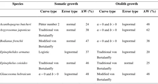
Table 3.1. Types of growth curves (and statistical distributions of errors) that, based on

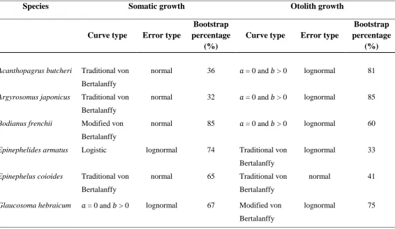
Akaike Information Criterion corrected for small sample size, best described total lengths and otolith radii at age of capture for Acanthopagrus butcheri, Argyrosomus japonicus, Bodianus frenchii, Epinephelides armatus, Epinephelus coioides and Glaucosoma hebraicum. 𝑎 and 𝑏 are parameters of the Schnute (1981) growth model. The modified von Bertalanffy curve has an oblique asymptote. AW = Akaike Weight………...p.68 Table 3.2. Types of growth curves (and statistical distributions of errors) that, based on

frequency of occurrence in bootstrap trials, best described total lengths and otolith radii at age of capture for Acanthopagrus butcheri, Argyrosomus japonicus, Bodianus frenchii,

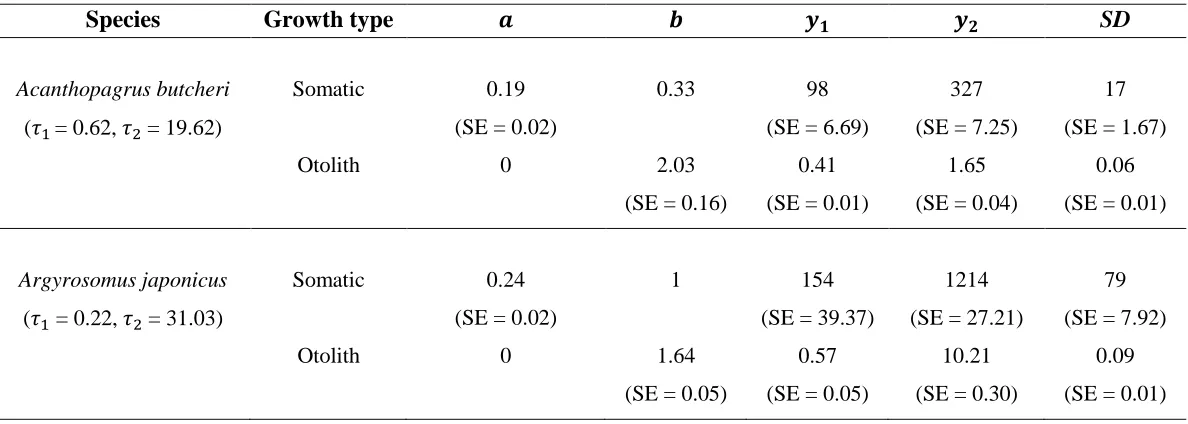
Epinephelides armatus, Epinephelus coioides and Glaucosoma hebraicum. Curve types are the same as described for Table 3.1. Bootstrap percentage = percentage of 4 000 trials for which the curve and error types were selected as best describing the bootstrap sample of lengths and ages at capture………p.69 Table 3.3. Values of parameters (𝑎, 𝑏, 𝑦₁and 𝑦₂) and standard deviations (SD) for Schnute (1981) (normal font) and modified von Bertalanffy (oblique linear asymptote, bold font) somatic and otolith growth curves of the fitted bivariate models for Acanthopagrus butcheri,

Argyrosomus japonicus, Bodianus frenchii, Epinephelides armatus, Epinephelus coioides and

Glaucosoma hebraicum. SD = estimated standard deviation of marginal distribution of deviations from the respective growth curve. Curves were the same as those of Table 3.1.

𝜏₁= first reference age (youngest fish in the sample), 𝜏₂= second reference age (oldest fish in the sample), 𝑎 and 𝑏 = parameters of growth model,𝑦₁ = size at age 𝜏₁, 𝑦₂= size at age 𝜏₂. Standard errors (SE) of the parameters and of the standard deviations are presented in

XIII Acanthopagrus butcheri, Argyrosomus japonicus, Bodianus frenchii, Epinephelides armatus,

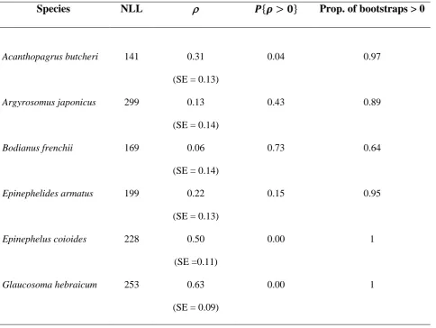
Epinephelus coioides and Glaucosoma hebraicum, together with correlation 𝜌 of the bivariate distribution of deviations from the somatic and otolith growth curves. Standard errors (SE) of the correlation are presented in parentheses. ‘𝑃{ > 0}’ = P-value of one-tailed t-test that

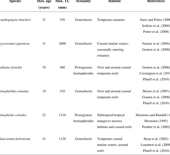
 > 0. ‘Prop. of bootstraps > 0’ = proportion of 4 000 bootstrap trials for which the point estimate of the correlation coefficient exceeded zero……….. p.72 Table S3.1. Maximum ages and total lengths (TL), sexuality, and habitats of Acanthopagrus

butcheri, Argyrosomus japonicus, Bodianus frenchii, Epinephelides armatus, Epinephelus

coioides and Glaucosoma hebraicum………..…… p.77

Table S3.2. Location and sampling regimes for Acanthopagrus butcheri, Argyrosomus japonicus, Bodianus frenchii, Epinephelides armatus, Epinephelus coioides and Glaucosoma hebraicum in estuarine and coastal waters along the western coast of Australia…………. p.79 Table S3.3. Birth dates assigned to each of Acanthopagrus butcheri, Argyrosomus japonicus,

Bodianus frenchii, Epinephelides armatus, Epinephelus coioides and Glaucosoma hebraicum

in estuarine and coastal waters along the coast of Western Australia………..… p.80 Table S3.4. The parameter space (a, b) for the Schnute (1981) growth curve was divided into nine regions such that, when fitting the model, parameters estimates could be constrained to each region. This avoided any discontinuity in derivatives that would have resulted if tests to determine whether to employ an equation with an alternative structure had been included in the Template Model Builder (TMB) code……… p.83 Table S3.5. Values of corrected Akaike Information Criteria (AICc) and Akaike Weights

XIV

assumed a normal distribution or lognormal distribution of deviations from expected lengths at age………..….. p.89 Table S3.6. Quantitatively similar somatic growth curves, i.e., curves with values of

corrected Akaike Information Criteria (AICc) lying within 2 units of the AICc (in bold font) of the best-fitting (i.e., lowest AICc) curve, for each of Acanthopagrus butcheri,

Argyrosomus japonicus, Bodianus frenchii, Epinephelides armatus, Epinephelus coioides and

Glaucosoma hebraicum………..… p.90

Table S3.7. Values of corrected Akaike Information Criteria (AICc) and Akaike Weights

(AWs) for otolith growth curves of different functional forms (i.e., a modified version of the von Bertalanffy growth equation and, for all other curve types, the versatile growth model described by Schnute (1981)) fitted to otolith radii (mm) at ages of capture for 50 individuals of Acanthopagrus butcheri collected from Wellstead Estuary in 2013, where the models assumed a normal distribution or lognormal distribution of deviations from expected radii at age……….…. p.91 Table S3.8. Quantitatively similar otolith growth curves, i.e., curves with values of corrected

Akaike Information Criteria (AICc) lying within 2 units of the AICc (in bold font) of the best-fitting (i.e., lowest AICc) curve, for each of Acanthopagrus butcheri, Argyrosomus japonicus, Bodianus frenchii, Epinephelides armatus, Epinephelus coioides and Glaucosoma

hebraicum………..……. p.92

Table S3.9. Values of adjusted coefficients of determination (𝑅_adjusted2 ) for the curves for total lengths and otolith radii at age of the fitted bivariate growth model for each of

Acanthopagrus butcheri, Argyrosomus japonicus, Bodianus frenchii, Epinephelides armatus,

XV

Table S3.10. Ranges of negative log-likelihoods (NLL) for the bivariate growth models

produced using the quantitatively similar somatic and otolith growth curves for

Acanthopagrus butcheri, Argyrosomus japonicus, Bodianus frenchii, Epinephelides armatus,

Epinephelus coioides and Glaucosoma hebraicum, together with ranges of both the

correlations (𝜌) between deviations from the growth curves for those bivariate models and the P-values, 𝑃{ > 0}, of one-tailed t-tests that those correlations exceed zero. Quantitatively similar curves were those with AICc scores lying within 2 units of the lowest score, i.e., the AICc of the fitted curve that best described the data……….… p.94

Table 4.1. Regression equations of the back-calculation approaches described by Morita and

Matsuishi (2001), Finstad (2003) and Vigliola and Meekan (2009), or derived from those equations……….…… p.128 Table 4.2. Regression equations, which pass through the biological intercept, modified (or

developed) from the equations of Morita and Matsuishi (2001), Finstad (2003) and Vigliola and Meekan (2009)……….…… p.129 Table 4.3a. Root Mean Square Error (RMSE) and mean error (ME) of total length estimates

for the bivariate growth model and models derived from the Morita and Matshuishi (2001) and Finstad (2003) models calculated using ten-fold cross-validations for samples of 50 fish for each of Acanthopagrus butcheri, Argyrosomus japonicus, Bodianus frenchii,

Epinephelides armatus, Epinephelus coioides, and Glaucosoma hebraicum. The percentages by which the RMSE of the alternative models differ from that of the bivariate growth model are presented in parentheses……….….. p.130 Table 4.3b. Root Mean Square Error (RMSE) and mean error (ME) of otolith radius

XVI

each of Acanthopagrus butcheri, Argyrosomus japonicus, Bodianus frenchii, Epinephelides armatus, Epinephelus coioides, and Glaucosoma hebraicum. The percentages by which the RMSE of the alternative models differ from that of the bivariate growth model are presented in parentheses……….…… p.131 Table 4.4a. Root Mean Square Error (RMSE) and mean error (ME) of total length estimates

for the bivariate growth model and for models derived from the Morita and Matshuishi (2001) and Finstad (2003) models calculated using holdout and ten-fold cross-validations with and without the biological intercept for samples of Acanthopagrus butcheri. The percentages by which the RMSE of the alternative models differ from that of the bivariate growth model are presented in parentheses……… p.132 Table 4.4b. Root Mean Square Error (RMSE) and mean error (ME) of total length estimates

for the bivariate growth model and the Morita and Matshuishi (2001) and the Finstad (2003) models calculated using holdout and ten-fold cross-validations with and without the

biological intercept for samples of Acanthopagrus butcheri. The percentages by which the RMSE of the alternative models differ from that of the bivariate growth model are presented in parentheses……….… p.133 Table 4.5. Mean observed total length (mm) and mean age of fish within each age class in

the 2013 sample of Acanthopagrus butcheri, together with mean back-calculated total lengths (mm) for fish at ages at zones bounding the age classes, calculated using different back-calculation approaches……….……... p.134-135

Table 5.1a. Corrected Akaike Information Criteria (AICc) for the fitted models (Eqs 1-5)

XVII

describing the relationships between the deviations, 𝑆𝑗,𝑎, at each pair of ages 𝑎1 and 𝑎2, and,

where present in the equations, the slopes (β) of those models……….…… p.163 Table 5.2. Corrected Akaike Information Criteria (AICc) for the fitted models (Eqs 6-8)

describing the relationships between the increment in otolith radius ∆𝑅𝑗,𝑡=𝑎+1 between

opaque zones a and a + 1 and the radius of the otolith at the first of these zones 𝑅_{𝑗,𝑡=𝑎}, and, where present in the equations, the intercepts (α) and slopes (β) of those relationships... p.165 Table S5.1. Akaike Weights (AWs) for the fitted models describing the relationships

between deviations, 𝑆_𝑗,𝑎, at each pair of ages 𝑎₁ and 𝑎₂ for fish j (1 ≤ 𝑗 ≤ 53) (Eqs 1-5, as shown in column headings) for 7-year-old Acanthopagrus butcheri from the Wellstead Estuary……… p.168-169 Table S5.2. Akaike Weights (AWs) for the fitted models (Eqs 6-8, as shown in column

headings) describing the relationships between the increment in otolith radius ∆𝑅_{𝑗,𝑡=𝑎+1} between opaque zones a and a + 1 for fish j (1 ≤ 𝑗 ≤ 53) and the radius of the otolith at the first of these zones 𝑅𝑗,𝑡=𝑎 for 7-year-old Acanthopagrus butcheri from the Wellstead

Estuary……….... p.170

Table 6.1. Maximum ages and total lengths (TL), sexuality, and habitats of Acanthopagrus

butcheri, Argyrosomus japonicus, Bodianus frenchii, Epinephelides armatus, Epinephelus coioides, and Glaucosoma hebraicum, the biological characteristics of which were employed in the simulation study………...… p.201 Table 6.2. Parameters from the ‘true’ somatic and otolith growth curves used to generate

simulated data for Acanthopagrus butcheri, Argyrosomus japonicus, Bodianus frenchii,

Epinephelides armatus, Epinephelus coioides, and Glaucosoma hebraicum……… p.202-203

Table 6.3. Parameters for the somatic and otolith growth curves of the bivariate growth

XVIII

employing a level of fishing mortality of F = 0.1 year-1 for Acanthopagrus butcheri,

Argyrosomus japonicus, Bodianus frenchii, Epinephelides armatus, Epinephelus coioides,

and Glaucosoma hebraicum………..…. p.204

Table 6.4. Parameters for the somatic and otolith growth curves of the bivariate growth

model fitted to samples of length and otolith size at age obtained through simulations employing a level of fishing mortality of F = 0.4 year-1 for Acanthopagrus butcheri,

Argyrosomus japonicus, Bodianus frenchii, Epinephelides armatus, Epinephelus coioides,

and Glaucosoma hebraicum………... p.205

Table 6.5. Parameters for the somatic and otolith growth curves of the bivariate growth

model fitted to samples of length and otolith size at age obtained through simulations employing a level of fishing mortality of F = 0.8 year-1 for Acanthopagrus butcheri,

Argyrosomus japonicus, Bodianus frenchii, Epinephelides armatus, Epinephelus coioides,

XIX

L

F

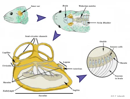
Figure 1.1. Schema of the location of the inner ear, its components and the innervation of the

otolith to the brain in teleost fish……… p.6

Figure 2.1. Sectioned otolith of a 262 mm Acanthopagrus butcheri from the Wellstead Estuary with seven opaque zones………. p.25 Figure 2.2. Left, photograph of the head of a two day-old Acanthopagrus butcheri larva, showing larval otoliths (identified by arrows); top-right, photograph of a whole

Acanthopagrus butcheri larva; bottom-right, extracted larval otolith………..…… p.28

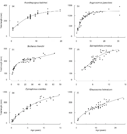
Figure 3.1. Growth curves fitted to the total lengths (mm) at ages of capture (years) for

Acanthopagrus butcheri, Argyrosomus japonicus, Bodianus frenchii, Epinephelides armatus,

Epinephelus coioides and Glaucosoma hebraicum………...…p.73

Figure 3.2. Growth curves fitted to the otolith radii (mm) at ages of capture (years) for

Acanthopagrus butcheri, Argyrosomus japonicus, Bodianus frenchii, Epinephelides armatus,

Epinephelus coioides and Glaucosoma hebraicum………..… p.74

Figure 3.3. Total lengths (mm) and otolith radii (mm) at capture for Acanthopagrus butcheri,

Argyrosomus japonicus, Bodianus frenchii, Epinephelides armatus, Epinephelus coioides and

Glaucosoma hebraicum, and the relationships formed by the pairs of values of total length and otolith radius at each age (over the range of observed ages at capture) predicted for each species using the somatic and otolith growth curves of the fitted bivariate growth model for that species……… p.75 Figure 3.4. Relative instantaneous rates of somatic and otolith growth versus age (years) at

capture for Acanthopagrus butcheri, Argyrosomus japonicus, Bodianus frenchii,

XX

represents somatic growth and dashed line (---) represents otolith growth…………..…… p.76 Figure S3.1. Quantitatively similar somatic growth curves, i.e., curves with AICc scores lying

within 2 units of the lowest score (the AICc of the best curve, in black), for Acanthopagrus butcheri, Argyrosomus japonicus, Bodianus frenchii, Epinephelides armatus, Epinephelus coioides and Glaucosoma hebraicum. Pütter = Pütter number 2, VB = traditional von Bertalanffy, ‘a=0, b>0’ = Schnute (1981) growth curve with a = 0 and b > 0, ModVB = modified von Bertalanffy, ND = normal distribution, LND = lognormal distribution…... p.95 Figure S3.2. Quantitatively similar otolith growth curves, i.e., curves with AICc scores lying

within 2 units of the lowest score (the AICc of the best curve, in black), for Acanthopagrus butcheri, Argyrosomus japonicus, Bodianus frenchii, Epinephelides armatus, Epinephelus coioides and Glaucosoma hebraicum. Pütter = Pütter number 2, VB = traditional von

Bertalanffy, GenVB = generalised von Bertalanffy, ‘a=0, b>0’ = Schnute (1981) growth curve with a = 0 and b > 0, ‘a<0, b>0’ = Schnute (1981) growth curve with a < 0 and b > 0, ModVB = modified von Bertalanffy……….… p.96 Figure S3.3. Relationships between total lengths and otolith radii at age formed by

quantitatively similar somatic and otolith growth curves for Acanthopagrus butcheri,

Argyrosomus japonicus, Bodianus frenchii, Epinephelides armatus, Epinephelus coioides and

Glaucosoma hebraicum. Black = best fitting somatic and otolith growth curves. Pütter = Pütter number 2, VB = traditional von Bertalanffy, GenVB = generalised von Bertalanffy, ‘a=0, b>0’ = Schnute (1981) growth curve with a = 0 and b > 0, ‘a<0, b>0’ = Schnute (1981) growth curve with a < 0 and b > 0, ModVB = modified von Bertalanffy, ND = normal

XXI

Figure 4.1.Comparison of mean observed total length (mm) versus mean age (years) of fish within each age class in the 2013 sample of Acanthopagrus butcheri, with the means of the total lengths (mm) at different ages at zones calculated using the different back-calculation approaches, i.e., the Bivariate Growth model (BG), the Age Effect model (AE) (i.e., the model described by Morita and Matsuishi (2001)), the Interaction Term model (IT) (i.e., model described by Finstad (2003)) and the Modified Fry model (MF) (i.e., model described by Vigliola et al. (2000)) with and without constraining the data through a biological

intercept (BI) for Acanthopagrus butcheri. 95% confidence intervals are represented as error bars. Note that data for the single fish at 21 years of age was excluded………….… p.136-137

Figure 5.1. Box and whisker plot of the deviations 𝑆_𝑗,𝑎 at each opaque zone. Mean values are given within each box, which represents the first two quartiles of data about the mean. Note that the mean is displayed rather than the more commonly used median. Standard deviations are displayed above the plotted data for each age………..… p.166 Figure 5.2. Scattergrams of the deviations for individual fish at each pair of opaque zones

(lower left triangle), histograms of deviations at each opaque zone (diagonal), and the correlations (and associated P-values) for the different pairs of opaque zones of individual fish (upper right triangle)………...… p.167

Figure 6.1. Mean ages (years) of fish within length slices (mm) at different levels of fishing

mortality (F = 0.1, 0.4 and 0.8 year-1) for Acanthopagrus butcheri, Argyrosomus japonicus,

Bodianus frenchii, Epinephelides armatus, Epinephelus coioides, and Glaucosoma

hebraicum………...… p.207

Figure 6.2. Differences between the mean ages (years) of fish within corresponding length

XXII

the sample produced for the fishing mortality F = 0.1 year-1, using a one-tailed Aspin-Welch t-test for Acanthopagrus butcheri, Argyrosomus japonicus, Bodianus frenchii, Epinephelides armatus, Epinephelus coioides, and Glaucosoma hebraicum. Solid black line represents mean ages at length for fish in the samples generated using F = 0.1 year-1, blue circles represent the comparison between mean ages at length for fish in the samples generated using F = 0.1 and 0.4 year-1, and red circles represent the comparison between mean ages at length for fish in the samples generated using F = 0.1 and 0.8 year-1. Large blue or red circles indicate the statistical significance (𝑃 < 0.05) of the comparisons……….…..… p.208-209 Figure 6.3. Mean ages (years) of fish within otolith radius slices (mm) at different levels of

fishing mortality (F = 0.1, 0.4 and 0.8 year-1) for Acanthopagrus butcheri, Argyrosomus japonicus, Bodianus frenchii, Epinephelides armatus, Epinephelus coioides, and Glaucosoma

hebraicum………...… p.210

Figure 6.4. Differences between the mean ages (years) of fish within corresponding otolith

radius (mm) classes for fishing mortalities, F = 0.4 and 0.8 year-1, and the mean age of the fish from the sample produced for the fishing mortality F = 0.1 year-1, using a one-tailed Aspin-Welch t-test for Acanthopagrus butcheri, Argyrosomus japonicus, Bodianus frenchii,

Epinephelides armatus, Epinephelus coioides, and Glaucosoma hebraicum. Solid black line represents mean ages at otolith radius for fish in the samples generated using F = 0.1 year-1, blue circles represent the comparison between mean ages at otolith radius for fish in the samples generated using F = 0.1 and 0.4 year-1, and red circles represent the comparison between mean ages at otolith radius for fish in the samples generated using F = 0.1 and 0.8 year-1. Large blue or red circles indicate the statistical significance (𝑃 < 0.05) of the

comparisons……… p.211-212 Figure 6.5. Mean otolith radius (mm) of fish within age (years) slices at increasing levels of

XXIII butcheri, Argyrosomus japonicus, Bodianus frenchii, Epinephelides armatus, Epinephelus

coioides, and Glaucosoma hebraicum………...… p.213

Figure 6.6. Mean otolith radius (mm) of fish within age (years) slices at increasing levels of

mean length at first capture (𝐿50) for a fishing mortality ofF = 0.8 year-1 for Acanthopagrus butcheri, Argyrosomus japonicus, Bodianus frenchii, Epinephelides armatus, Epinephelus

coioides, and Glaucosoma hebraicum………...…… p.214

Figure 6.7. Differences between the mean otolith radius (mm) of fish within corresponding

age (years) classes for larger values of 𝐿₅₀ and the mean otolith size of the fish from the sample produced for the smaller values of 𝐿₅₀, using a one-tailed Aspin-Welch t-test for

Acanthopagrus butcheri, Argyrosomus japonicus, Bodianus frenchii, Epinephelides armatus,

Epinephelus coioides, and Glaucosoma hebraicum at the highest fishing mortality,

F = 0.8 year-1. Solid black line represents mean otolith radii at age for fish in the samples generated using the smaller values of 𝐿50 and red circles represent the comparison between

mean otolith radii at age for fish in the samples generated using the larger and the smaller values of 𝐿₅₀. Large red circles indicate the statistical significance (𝑃 < 0.05) of the

comparisons………...……….… p.215-216 Figure 6.8. Mean length (mm) of fish within otolith radius slices (mm) at different levels of

fishing mortality (F = 0.1, 0.4 and 0.8 year-1) for Acanthopagrus butcheri, Argyrosomus japonicus, Bodianus frenchii, Epinephelides armatus, Epinephelus coioides, and Glaucosoma

hebraicum………...…… p.217

Figure 6.9. Differences between the mean length (mm) of fish within corresponding otolith

radius (mm) classes for fishing mortalities, F =0.4 and 0.8 year-1, and the mean length of the fish from the sample produced for the fishing mortality F = 0.1 year-1, using a one-tailed Aspin-Welch t-test for Acanthopagrus butcheri, Argyrosomus japonicus, Bodianus frenchii,

XXIV

represents mean lengths at otolith radius for fish in the samples generated using

F = 0.1 year-1, blue circles represent the comparison between mean lengths at otolith radius for fish in the samples generated using F = 0.1 and 0.4 year-1, and red circles represent the comparison between mean lengths at otolith radius for fish in the samples generated using

F = 0.1 and 0.8 year-1. Large blue or red circles indicate the statistical significance

(𝑃 < 0.05) of the comparisons………...…… p.218-219

Figure 6.10. Mean otolith radius (mm) of fish within length slices (mm) at different levels of

fishing mortality (F = 0.1, 0.4 and 0.8 year-1) for Acanthopagrus butcheri, Argyrosomus japonicus, Bodianus frenchii, Epinephelides armatus, Epinephelus coioides, and Glaucosoma

hebraicum………...… p.220

Figure 6.11. Differences between the mean otolith radius (mm) of fish within corresponding

length (mm) classes for fishing mortalities, F = 0.4 and 0.8 year-1, and the mean otolith radius of the fish from the sample produced for the fishing mortality F = 0.1 year-1, using a one-tailed Aspin-Welch t-test for Acanthopagrus butcheri, Argyrosomus japonicus, Bodianus frenchii, Epinephelides armatus, Epinephelus coioides, and Glaucosoma hebraicum. Solid black line represents mean otolith radii at length for fish in the samples generated using

F = 0.1 year-1, blue circles represent the comparison between mean otolith radii at length for fish in the samples generated using F = 0.1 and 0.4 year-1, and red circles represent the comparison between mean otolith radii at length for fish in the samples generated using

F = 0.1 and 0.8 year-1. Large blue or red circles indicate the statistical significance

(𝑃 < 0.05) of the comparisons………...… p.221-222

Figure 6.12. Length (mm) at age (years) calculated using the ‘true’ growth curves and

predicted using the bivariate growth model at different levels of fishing mortality (F = 0.1, 0.4 and 0.8 year-1) for Acanthopagrus butcheri, Argyrosomus japonicus, Bodianus frenchii,

XXV

Figure 6.13. Otolith radius (mm) at age (years) calculated using the ‘true’ growth curves and

predicted using the bivariate growth model at different levels of fishing mortality (F = 0.1, 0.4 and 0.8 year-1) for Acanthopagrus butcheri, Argyrosomus japonicus, Bodianus frenchii,

Epinephelides armatus, Epinephelus coioides, and Glaucosoma hebraicum……… p.224

Figure 6.14. Length (mm) at otolith radius (mm) calculated using the ‘true’ growth curves

and predicted using the bivariate growth model at different levels of fishing mortality (F = 0.1, 0.4 and 0.8 year-1) for Acanthopagrus butcheri, Argyrosomus japonicus, Bodianus frenchii, Epinephelides armatus, Epinephelus coioides, and Glaucosoma hebraicum.…. p.225

Figure 6.15. Distribution of length (mm) deviations with age (years) from the ‘true’ somatic

growth curve at the lowest level of fishing mortality, F = 0.1 year-1, for Acanthopagrus butcheri, Argyrosomus japonicus, Bodianus frenchii, Epinephelides armatus, Epinephelus

coioides, and Glaucosoma hebraicum………..….… p.226

Figure 6.16. Distribution of otolith radius (mm) deviations with age (years) from the ‘true’

otolith growth curve at the lowest level of fishing mortality, F = 0.1 year-1, for

Acanthopagrus butcheri, Argyrosomus japonicus, Bodianus frenchii, Epinephelides armatus,

Epinephelus coioides, and Glaucosoma hebraicum………...… p.227

Figure 6.17. Distribution of length (mm) deviations with age (years) from the ‘true’ somatic

growth curve at the highest level of fishing mortality, F = 0.8 year-1, for Acanthopagrus butcheri, Argyrosomus japonicus, Bodianus frenchii, Epinephelides armatus, Epinephelus

coioides, and Glaucosoma hebraicum………...…… p.228

Figure 6.18. Distribution of otolith radius (mm) deviations with age (years) from the ‘true’

otolith growth curve at the highest level of fishing mortality, F = 0.8 year-1, for

Acanthopagrus butcheri, Argyrosomus japonicus, Bodianus frenchii, Epinephelides armatus,

Epinephelus coioides, and Glaucosoma hebraicum………...… p.229

XXVI

of fishing mortality (F = 0.1, 0.4 and 0.8 year-1) for Acanthopagrus butcheri, Argyrosomus japonicus, Bodianus frenchii, Epinephelides armatus, Epinephelus coioides, and Glaucosoma

hebraicum………...… p.230

Figure S6.2. Fish length (mm) compositions of the fish in simulated samples at different

levels of fishing mortality (F = 0.1, 0.4 and 0.8 year-1) for Acanthopagrus butcheri,

Argyrosomus japonicus, Bodianus frenchii, Epinephelides armatus, Epinephelus coioides,

and Glaucosoma hebraicum………...… p.231

Figure S6.3. Otolith radius (mm) compositions of the fish in the simulated samples at

different levels of fishing mortality (F = 0.1, 0.4 and 0.8 year-1) for Acanthopagrus butcheri,

Argyrosomus japonicus, Bodianus frenchii, Epinephelides armatus, Epinephelus coioides,

and Glaucosoma hebraicum………...… p.232

Figure S6.4. Age (years) compositions of the fish in the simulated samples at two levels of

mean length at first capture (𝐿₅₀) for a fishing mortality ofF = 0.8 year-1 for Acanthopagrus butcheri, Argyrosomus japonicus, Bodianus frenchii, Epinephelides armatus, Epinephelus

coioides, and Glaucosoma hebraicum………...…… p.233

Figure S6.5. Fish length (mm) compositions of the fish in the simulated samples at two

levels of mean length at first capture (𝐿50) for a fishing mortality ofF = 0.8 year-1 for

Acanthopagrus butcheri, Argyrosomus japonicus, Bodianus frenchii, Epinephelides armatus,

Epinephelus coioides, and Glaucosoma hebraicum………...… p.234

Figure S6.6. Otolith radius (mm) compositions of the fish in the simulated samples at two

levels of mean length at first capture (𝐿₅₀) for a fishing mortality ofF = 0.8 year-1 for

Acanthopagrus butcheri, Argyrosomus japonicus, Bodianus frenchii, Epinephelides armatus,

XXVII

Figure SA. Sectioned otoliths of the six study species, showing the location of the radius (red

line) from the primordium to the outer edge of the otolith, to the right of the sulcus and perpendicular to the opaque zones. Scale bar = 1 mm………...…… p.248 Figure SB. Whole otoliths of adults and juveniles for the six study species. Scale

1

C

1

–

G

I

1.1

B

Back-calculation is an important tool in fisheries science and fish ecology for

reconstructing growth histories of individual marine organisms based on the microstructure present within calcified structures such as statoliths, vertebrae and otoliths. For teleosts, the most commonly used hard structures in back-calculation studies are their otoliths, presumably because the results of numerous fish age validation studies have shown that these structures can be used to accurately determine the ages of individual fish, and thereby also facilitate reliable determination of their growth. Although back-calculation studies also rely on an accurate description of the relationship between fish length and otolith size, the factors that can influence this relationship remain poorly understood. Furthermore, current studies of back-calculation typically provide no link between traditional somatic growth models and their relationship to otolith growth. To address this omission, I developed a growth model that describes both somatic and otolith growth using traditional forms of growth curves and, assuming a bivariate distribution of deviations from these two growth curves, also relates fish lengths at age to otolith size. The performance of this model was compared with existing approaches using data for six fish species with widely varying biological characteristics. The bivariate growth model was then extended to produce a proportionality-based

2

Finally, the effects of fishing mortality and length-dependent selectivity on mean and

predicted otolith sizes at age and on the relationship between fish length and otolith size, the basis of all back-calculation approaches, were explored.

1.2

S

Otoliths are hard calcium carbonate structures found in pairs within the heads of all teleosts, and are employed for balance, orientation and hearing (e.g., Campana and Neilson 1985; Campana 1999). The main interest that otoliths hold for biologists and fishery scientists lies in the fact that these structures store valuable information on age of fishes and the

environment within which they lived at different ages throughout life, facilitating

understanding of population dynamics, stock identity, fish systematics and evolution (Popper et al. 2005). The use of otoliths as indicators of fish age began with Reibisch’s (1899)

observations of otolith annuli in Pleuronectes platessa. Since then, interest in otolith microstructure as a metabolically-inert timekeeper and environmental recorder has grown exponentially, with close to a million fish aged each year worldwide (Campana et al. 2000; Campana and Thorrold 2001; Campana 2005).

The information related to growth and environment contained within the otolith

3

annual intervals are used to determine the ages individual fish for estimating growth, longevity, and mortality rates in fish populations (e.g., Campana 2001; Wilson and Nieland 2001; Laidig et al. 2003). This understanding of fish population biology is vital for producing reliable fish stock assessments required for determining effective management strategies to allow fish harvesting whilst ensuring that the risk of such harvesting to the long term

sustainability of the stock remains at an appropriate level (Jones 1992; Campana 2001; Begg et al. 2005).

4

includes several historical models as special cases, and which can be related to both accelerated and decelerated growth.

A prominent application of otolith microstructure examination is growth back-calculation, which involves estimating the length of individual fish at successive ages throughout life (e.g., Francis 1990; Campana and Jones 1992). Back-calculation is an invaluable analytical method widely used in fisheries science and ecology around the world for reconstructing individual growth histories of teleosts (e.g., Francis 1990; Campana 2005; Vigliola and Meekan 2009). The most common application of back-calculation is that of complementing the observations of lengths at the ages of capture with estimates of lengths at age for younger fish. Curves are then fitted to the combined set of observations and estimates to determine values of key growth parameters (e.g., the asymptotic length or the growth coefficient of the von Bertalanffy growth function) and to compare, describe or predict growth variations among individuals (e.g., Shafi and Jasim 1982; Jones 2000; Colloca et al. 2003; Lorance et al. 2003; Ballagh et al. 2011). For some species, growth histories within bony structures, such as otoliths, become particularly useful when samples sizes are small or information on life history at earlier ages is lacking (e.g., Campana 1989; Meekan et al. 1998a; Vigliola and Meekan 2009). Growth curves derived from back-calculated data have been used to compare growth rates between sexes, cohorts and populations of the same species (e.g., Frost and Kipling 1980; Thorrold and Williams 1989; Sirois et al. 1998;

5

variation of size-selective mortality on previous life history stages (e.g., Grønkjær and Schytte 1999; Good et al. 2001; Sinclair et al. 2002a).

Another common application of information from otoliths is the use of otolith microchemistry for discriminating fish stocks and understanding population connectivity (e.g., Gillanders 2002; Rooker et al. 2003; Fowler et al. 2005; Stransky et al. 2005; Thresher and Proctor 2007). Environmental histories and migration patterns and/or habitat shifts throughout the lives of individual fish have been reconstructed from otolith elemental concentrations, which change in a predictable manner with environmental variables (e.g., Elsdon and Gillanders 2004; Daverat et al. 2005; Dorval et al. 2005; Hobbs et al. 2005). Furthermore, techniques developed initially for analysing tree-ring data (i.e.,

dendrochronology) have been employed to describe the long-term relationships between trends exhibited by otolith growth and aspects of environmental variability (e.g., water temperature) (e.g., Black 2009; Neuheimer et al. 2011; Gillanders et al. 2012; Black et al. 2013). Sclerochronology, or the study of calcified structures to reconstruct the past history of living organisms, which employs these relationships to predict the effects of climate change from otolith biochronologies, is becoming an important aspect of fisheries management (e.g., Panfili et al. 2002; Matta et al. 2010; Gillanders et al. 2012).

1.3

O

,

Otoliths play the role of a mechanoreceptor (e.g., involvement with the maintenance of equilibrium, the detection of gravity and sound) in the inner ear of fish. The nerve cells in the macula (a sensory epithelium which lies close to the otolith) of the labyrinth organ are

6

the sacculus) connected by three semi-circular canals, filled with endolymph (an acellular medium similar in constitution to plasma and secreted by the inner ear epithelium) and containing one otolith each, i.e., the asteriscus, the lapillus and the sagitta (Lowenstein 1956; Enger 1964; Payan et al. 2004) (see Fig. 1.1). The sagittae, the largest of the three pairs of otoliths, are used by fish for directional hearing and frequency responses (Lu and Xu 2002), while the lapilli are predominantly involved in balance and orientation (Riley and Moorman 2000).

Figure 1.1. Schema of the location of the inner ear, its components and the innervation of the

otolith to the brain in teleost fish.1

1

The illustration, which was drawn by the author, was inspired from different sources, namely - Drawing of the left Merluccius spp. inner ear by A. Lombarte (see Morales-Nin 2000)

- ‘Sensory systems’ refer tohttp://www.snre.umich.edu/~pwebb/NRE422-BIO440/lec16.html (viewed on 16/02/2016) - ‘Illustration of the anatomy of the inner ear of fish’ by C. Iverson

7

The acellular and metabolically inert nature of otoliths enables elements or compounds to accrete onto their surface and to be permanently retained, while continued otolith growth from before hatching to death records the entire life of the fish (Campana and Neilson 1985). The general pathway of inorganic elements into the otolith is from water into the blood plasma via osmoregulation in the gills (in freshwater fish) or the intestine (in saltwater fish), then into the endolymph and, lastly, into the crystallising otolith (Olsson et al. 1998; Campana 1999).

Otolith composition is dominated by calcium carbonate (99% CaCO3 in the aragonite

form) deposited onto a non-collagenous organic matrix (e.g., Asano and Mugiya 1993; Hoff and Fuiman 1993; Campana 1999; Payan et al. 2004). The calcification process (i.e., the deposition of mineral) is mainly dependent on the composition of the endolymphatic fluid surrounding the otolith and can thus be described on the basis of physical principles, one of the key regulating factors being the pH of the endolymph (Romanek and Gauldie 1996; Payan et al. 1997, 1998, 2004; Campana 1999). The gradient of the pH, determined by the concentration of bicarbonate ions within the endolymph and resulting from high to low levels of metabolic activity, maintains the gradient in otolith calcification (Mugiya 1986; Gauldie and Nelson 1990a; Mugiya and Yoshida 1995; Payan et al. 2004). Since otolith growth is a biomineralisation process, the proteins, which represent a small percentage of the otolith and constitute the organic matrix, also play a pivotal role in the calcification process (e.g.,

Wheeler and Sikes 1984; Campana 1999). While water-insoluble otolith proteins constitute the structural framework of calcification, it is the water-soluble, calcium-binding proteins which regulate the rate of calcification and the type of calcium carbonate crystals which are formed (Wright 1991; Asano and Mugiya 1993; Campana 1999).

8

otolith, growth increments are laid down through differential deposition of calcium carbonate (translucent concentric rings) and protein (opaque concentric rings) (Campana and Neilson 1985; Mugiya 1987; Gauldie and Nelson 1988). At the endogenous level, the proteins of the organic matrix regulate the rate of calcification and thus otolith growth (Wheeler and Sikes 1984; Wright 1991; Asano and Mugiya 1993). The periodicity of increment formation follows endogenous diel rhythms, entrained by photoperiod and synchronised to periodic environmental cycles, which characterise the neural activity of most animals (Campana and Neilson 1985; Gauldie and Nelson 1988). Since Pannella’s (1971) discovery of daily growth increments, the circadian rhythm of calcium deposition has been shown to be controlled by endocrinological processes (e.g., Boeuf and Le Bail 1999; Shiao et al. 2008). Another important control and the main environmental factor affecting otolith growth rate is water temperature, which has been found to regulate the rate of calcification (e.g., Gutiérrez and Morales-Nin 1986; Mosegaard and Titus 1987;Mosegaard et al. 1988; Lombarte and Lleonart 1993; Folkvord et al. 2004). Subsequently, both the anatomy and function of the inner ear, together with environmental conditions (conveyed through physiological processes) regulate, otolith growth rates.

Note that in the present study, the term ‘otolith growth’ relates to the accretion of mineral onto the organic matrix of the otolith, rather than referring to growth in terms of cellular division.

1.4

S

9

rate of somatic growth is directly proportional to the rate of otolith growth. Such an assumption also underpins most back-calculation methods (e.g., Campana 1990; Francis 1990; Sirois et al. 1998; Vigliola et al. 2000; Morita and Matsuishi 2001).

The rate of protein synthesis in fish is associated with metabolic rate, somatic growth rate and temperature (Mommsen 2001; Pörtner et al. 2001). As somatic growth reflects the rate of net protein synthesis, the rate of formation of a proteinaceous matrix on the surface of a growing otolith is consequently highly correlated with the rate of somatic growth (Campana 1999). In an experiment on the effect of a short period of starvation between two groups of rainbow trout (Oncorhynchus mykiss), Payan et al. (1998) selected starvation as a natural physiological situation characterised by a reduction in both somatic and otolith growth. A reduction in the rate of otolith growth in a group of starved trout was directly related to an overall decline in the alkalinity of the endolymph which, in turn, is known to be dependent on the acid-base balance in teleosts (Payan et al. 1997; Payan et al. 1998). Furthermore, as ~ 10-30% of otolith carbon can be derived from metabolism, isotopic composition of otoliths can be used to trace changes in metabolic activity throughout the life of fish, with a tendency for protein synthesis and otolith growth to decline with age (Mulcahy et al. 1979; Schwarcz et al. 1998). Through this effect of metabolism on otolith growth, variation in somatic growth will be reflected, to some extent, in otolith microstructure, implying that increment width

trajectory, i.e., along a line perpendicular to the widths between successive growth zones from the centre to the outer edge of the otolith, can provide information on changes in somatic growth (e.g., Thorrold and Williams 1989; Wang and Tzeng 1999; Oozeki and Watanabe 2000; Fey 2006).

10

general theory which relates otolith growth to metabolic rate (influenced by temperature, food intake, dominance status and other activity cycles), rather than somatic growth rate (e.g., Mosegaard et al. 1988; Wright et al. 1990; Titus and Mosegaard 1991; Wright 1991; Metcalfe et al. 1992; Yamamoto et al. 1998; Folkvord et al. 2004; Fey 2005). Consequently, changes in otolith increment width may not be well linked to variation in somatic growth, and

particularly when otolith and somatic growths are affected by short-term fluctuations in temperature or food (e.g., Bradford and Geen 1992; Barber and Jenkins 2001). It is important to note, however, that otolith growth continuously scales to somatic growth in an

age-dependent manner (Secor and Dean 1992). Variations in the strength of the relationship between otolith and somatic growth may also reflect the effects of measurement error associated with differing measures of otolith size and, in linear regression analyses, reduced contrast associated with the compression of the range of fish sizes as a result of, for example, size-selective mortality (Meekan et al. 1998a, b).

11

processes involved in daily physiological cycles, i.e., an ‘age effect’ (e.g., Mosegaard et al. 1988; Gauldie and Nelson 1990a; Secor and Dean 1992; Morales-Nin 2000). Indeed, while the rate of organic matrix formation might provide threshold limits for calcification rate in otoliths, the effect of temperature may promote calcification rate within those limits (Mosegaard et al. 1988; Campana 1999). Both the age and growth effects are linked, as continued increase in otolith size can induce disproportionately larger otoliths in slow-growing individuals than those of fast-slow-growing fish of the same size (Mosegaard et al. 1988; Secor and Dean 1989; Wright et al. 1990; Fey 2006). The growth effect may also vary through time and therefore introduce curvature into otolith size trajectories for individual fish, as growth varies over time and particularly among ontogenetic stages (Campana 1990). In a simulation, Campana (1990) demonstrated that individual variability in growth rates induced bias into the fish-otolith size relationship and could thus explain Lee’s Phenomenon, i.e., back-calculated lengths are smaller than observed lengths at age at capture.

The terms ‘uncoupling’, ‘decoupling’ and other such terminologies have been poorly defined in previous studies of the relationship between somatic and otolith growth rates and are likely to be inaccurate (Secor and Dean 1992; Xiao 1996). Their continued usage seems to serve the purpose of separating the specific problem of the relationship between somatic and otolith growth from the general context of allometry and from the basic assumptions of back-calculation (Hare and Cowen 1995). In this thesis, and as suggested by Xiao (1996), the relationships between somatic and otolith growth rates will be described through the life of fish.

1.5

B

-

12

the otolith edge, to deduce body lengths for an individual fish at ages prior to capture, while assuming that there is a relationship between the length and otolith size at capture and the measured sizes (Carlander 1981; Campana 1990; Hare and Cowen 1995; Sirois et al. 1998; Vigliola et al. 2000; Morita and Matsuishi 2001; Vigliola and Meekan 2009).

Back-calculation requires 1) that the periodic deposition rate of increments is constant within the otolith (Geffen 1992); 2) that these increments can be read with accuracy and precision (Campana 1992); and 3) that there is a relationship between somatic and otolith growth of fish, which is derived from strong correlations between body size of fish and otolith size (Francis 1990; Vigliola and Meekan 2009). Field and experimental evidence as to partial “uncoupling” between somatic and otolith growth rates (e.g., Mosegaard et al. 1988; Secor and Dean 1989; Wright et al. 1990; Fey 2006) may thus directly challenge the capability of back-calculation to produce reliable estimates of fish length. Indeed, because the effects of age and growth are not mutually exclusive (Morita and Matsuishi 2001), both factors can introduce biases into the fish length-otolith relationship and thus invalidate back-calculation. To avoid potential bias associated with back-calculation, rather than predicting lengths at age of young fish using this approach, some authors employ otolith radius at age as a proxy for length at age when studying growth (Hare and Cowen 1995). Such an approach would avoid bias due to the effect of size-selective mortality on the fish-otolith size relationship (Ricker 1969; Gleason and Bengtson 1996; Grimes and Isely 1996). Recent experimental and theoretical findings, however, have strongly refuted this approach and results demonstrated that, for some species, back-calculated size at age is a better proxy of fish length at age than otolith radius at age (Wilson et al. 2009).