The Green tensor of Mindlin’s anisotropic first strain gradient elasticity

O R I G I N A L A R T I C L E

Open Access

The Green tensor of Mindlin’s

anisotropic first strain gradient elasticity

Giacomo Po

, Nikhil Chandra Admal

and Markus Lazar

*Correspondence:gpo@ucla.edu 1_{Department of Mechanical and} Aerospace Engineering, University of California Los Angeles, Los Angeles 90095, CA, USA 2_{Department of Mechanical and} Aerospace Engineering, University of Miami, Coral Gables 33146, FL, USA

Full list of author information is available at the end of the article

Abstract

We derive the Green tensor of Mindlin’s anisotropic first strain gradient elasticity. The Green tensor is valid for arbitrary anisotropic materials, with up to 21 elastic constants and 171 gradient elastic constants in the general case of triclinic media. In contrast to its classical counterpart, the Green tensor is non-singular at the origin, and it converges to the classical tensor a few characteristic lengths away from the origin. Therefore, the Green tensor of Mindlin’s first strain gradient elasticity can be regarded as a physical regularization of the classical anisotropic Green tensor. The isotropic Green tensor and other special cases are recovered as particular instances of the general anisotropic result. The Green tensor is implemented numerically and applied to the Kelvin problem with elastic constants determined from interatomic potentials. Results are compared to molecular statics calculations carried out with the same potentials.

Keywords: Green tensor, Gradient elasticity, Anisotropy, Non-singularity, Kelvin problem

Introduction

Green functions are objects of fundamental importance in field theories, since they rep-resent the fundamental solution of linear inhomogeneous partial differential equations (PDEs) from which any particular solution can be obtained via convolution with the source term (Green1828). Moreover, Green functions are the basis of important numeri-cal methods for boundary value problems, such as the boundary element method (Becker 1992), and they provide “flexible" boundary conditions for atomistic simulations (Trinkle 2008). In the context of linear elasticity, the Green function is a tensor-valued function of rank two, also known as the Green tensor. When contracted with a concentrated force acting at the origin, the Green tensor yields the displacement field in an infinite elastic medium. Kelvin (1882) first derived the closed-form expression of the classical Green ten-sor for isotropic materials. For anisotropic materials, Lifshitz and Rosenzweig (1947) and Synge (1957) were able to derive the Green tensor in terms of an integral expression over the equatorial circle of the unit sphere in Fourier space. Barnett (1972) extended this result to the first two derivatives of the Green tensor, and showed that the line-integral repre-sentation is well suited for numerical integration (see also Bacon et al. (1979); Teodosiu (1982)).

The Green tensor and its derivatives are singular at the origin, ultimately as a con-sequence of the lack of intrinsic length scales in the classical theory of elasticity. The

unphysical singularities in the elastic fields derived from the Green tensor hinder their applicability in nano-mechanics, including the elastic theory of defects such as cracks, dislocations and inclusions (Mura 1987; Askes and Aifantis 2011). Generalized elastic field theories with intrinsic length scales have been proposed in the context of micro-continuum theories (Eringen 1999), non-local theories (Eringen 2002), and gradient theories (Kröner1963; Mindlin1964; 1968b; 1972; Mindlin and Eshel1968a). In par-ticular, Mindlin’s anisotropic strain gradient elasticity has received renewed attention as a tool to solve engineering problems at the micro- and nano-scales for realistic materi-als (Polizzotto2018). Only recently, the structure of the gradient-elastic tensor has been rationalized for different material symmetry classes (Auffray et al.2013), and its atom-istic representation and ensuing determination from interatomic potentials has become available (Admal et al.2016).

The number of independent strain gradient elastic moduli ranges from 5 for isotropic materials, to 171 in the general case of triclinic materials. While simple expressions of the Green tensor exist for the isotropic case (Rogula 1973; Lazar and Po 2018), and for simplified anisotropic theories (Lazar and Po 2015a, b), the Green tensor of the fully anisotropic theory of Mindlin’s strain gradient elasticity has remained so far a rather elusive object. Rogula (1973) provided an expression for the Green tensor in gradient elasticity of arbitrary order, which involves a sum of terms associated with the roots of a certain characteristic polynomial. However, such representation renders its numerical implementation rather impractical, and it con-ceals the mathematical structure of the Green tensor in relationship to its classical counterpart.

The objective of this paper is to derive a simple representation of the Green tensor of Mindlin’s anisotropic first strain gradient elasticity, whose integral kernel involves only matrix operations suitable for efficient numerical implementation. Following a brief summary of Mindlin’s anisotropic first strain gradient elasticity, we derive the matrix representation of the Green tensor. It is shown that the Green tensor is non-singular at the origin, while its first gradient is finite but discontinuous at the origin. The classical tail of the Green tensor, as well as its classical limit for vanishing gra-dient parameters are easily recovered from the non-singular expression. We demon-strate that the Green tensor generalizes other expressions found in the literature, and finally consider the Kelvin problem where the Green tensor is compared to atomistic calculations.

Mindlin’s anisotropic gradient elasticity

Let us consider an infinite elastic body in three-dimensional space and assume that the gradient of the displacement fielduis additively decomposed into an elastic distortion tensorβand an inelastic1eigen-distortion tensorβ∗:

∂jui=βij+βij∗. (1)

W(e,∇e)= 1

2Cijkleijekl+ 1

2Dijmkln∂meij∂nekl. (2)

The strain energy density (2) is a function of the infinitesimal elastic strain tensor

eij=

1 2

βij+βji, (3)

and of its gradienteij,m. The tensorCis the standard rank-four tensor of elastic constants.

By virtue of the symmetries

Cijkl =Cjikl=Cijlk =Cklij, (4)

it possesses up to 21 independent constants with units of eV/Å3. The tensor Dis the rank-six tensor of strain gradient elastic constants, with symmetries

Dijmkln=Djimkln=Dijmlkn=Dklnijm. (5)

It has units of eV/Å. In the general case of triclinic materials the number of independent constants in the tensorDis equal to 171 (Auffray et al.2013).

The quantities conjugate to the elastic strain tensor and its gradient are the Cauchy stress tensorσand the double stress tensorτ, respectively. These are defined as:

σij= ∂_∂W

eij =Cijkl

ekl, (6)

τijm= ∂W

∂(∂meij) = Dijmkln

ekl,n. (7)

In the presence of a body forces densityb, the static Lagrangian density of the system becomes:

L= −W−V= −1 2

Cijklβijβkl+Dijmklnβij,mβkl,n

+uibi, (8)

where

V= −uibi (9)

is the potential of the body force. The condition of static equilibrium is expressed by the Euler-Lagrange equation

δL δui =

∂L ∂ui −∂j

∂L

∂(∂jui) +∂k∂j ∂L ∂(∂k∂jui) =

0 . (10)

In terms of the Cauchy and double stress tensors, Eq. (10) takes the following form (Mindlin1964):

∂j

σij−∂mτijm

+bi=0 . (11)

Using Eqs. (1) (6) (7), Eq. (11) can be cast in the following equation for displacements:

LM_ikuk+fi=0 . (12)

In Eq. (12),LM_ik denotes the differential operator of Mindlin’s anisotropic first strain gradient elasticity

LM_ik =Cijkl∂j∂l−Dijmkln∂j∂l∂m∂n, (13)

while

fi=bi−

Cijkl∂j−Dijmkln∂j∂m∂n

β_kl∗ (14)

of material defects, such as inclusions, cracks, and dislocations. This term is the gradient version of the internal force in Mura’s eigen-strain theory (Mura1987).

The Green tensor of Mindlin’s first strain gradient elasticity

In this section, we derive the three-dimensional Green tensor of the operator (13). To this end, we seek the solution to Eq. (12) in the form

uk =Gkj∗fj, (15)

where the symbol∗indicates convolution over the three-dimensional space, andGis the Green tensor of Mindlin’s anisotropic differential operatorLM. Substituting Eq. (15) into Eq. (12), one finds thatGsatisfies the following inhomogeneous PDE:

Cijkl∂j∂l−Dijmkln∂j∂l∂m∂n

Gkm+δimδ=0 . (16)

In Eq. (16), δij is the Kronecker symbol, while δ is the three-dimensional Dirac δ-distribution.

Taking the Fourier transform3of Eq. (16), we obtain the following algebraic equation for the Green tensorGˆkj(k)in Fourier space

[Cik(k)+Dik(k)]Gˆkj(k)=δij, (17)

where

Cik(k)=Cijklkjkl, (18)

Dik(k)=Dijmklnkjklkmkn (19)

are symmetric matrices. If we further define the unit vector in Fourier space

κ = k

k, k=

kiki, κ2=1 , (20)

then (17) becomes:

k2Cik(κ)+k2Dik(κ) _ˆ

Gkj(k)=δij, (21)

or equivalently, in matrix notation,

k2C(κ)+k2D(κ)Gˆ(k)=I. (22) Stability of the differential operatorLMrequires that the matrixC(κ)+k2_D(κ)be pos-itive definite. Since this requirement must hold for allk andκ, then the matricesC(κ) andD(κ) must be individually positive definite. Under the assumption thatC(κ)and

D(κ)are symmetric positive definite (SPD) matrices, the solution of (22) in Fourier space clearly reads:

ˆ

G(k)=

C(κ)+k2D(κ)−1

k2 . (23)

The three-dimensional Green tensor in real space is obtained by inverse Fourier transform of Eq. (23). It reads:

G(x)= 1 8π3

R3

C(κ)+k2D(κ)−1

k2 cos(k·x) dVˆ

= 1 8π3

S

∞

0

In Eq. (24), dVˆ =k2dkdωindicates the volume element in Fourier space, and dωis an elementary solid angle on the unit sphereS. Our objective now is to obtain an alternative expression of the matrix inverse [C(κ)+k2D(κ)]−1which allows us to carry out the the

k-integral analytically. By doing so, the non-singular nature of the Green tensor at the origin is revealed. We start by observing that, by virtue of its SPD character, the matrix

C(κ)admits the following eigen-decomposition

C(κ)=R(κ)V2(κ)RT(κ), (25)

where R(κ) is the orthogonal matrix of the eigenvectors of C(κ), while V2(κ) is the diagonal matrix of positive eigenvalues ofC(κ). Moreover, the matrix

C12 =_R(κ)_V(κ)_RT(κ) (26)

is also SPD. Using (26), let us consider the following identity:

C+k2D(κ)=C12_I+_k22(κ)C12_{, (27)} where

2_(κ)=C−1_2(κ)D(κ)C−1_{2(κ) (28)}

is a SPD matrix with units of length squared. With this decomposition, the Green tensor in Fourier space becomes

ˆ

G(k)=C−12(κ)

I+k22(κ)−1 k2 C

−1

2(κ)_{, (29)}

while in real space we obtain

G(x)= 1 8π3

SC

−1 2(κ)

_∞

0

I+k22(κ)−1cos(kκ·x)dkC−12(κ)dω. (30) In order to carry out thek-integral, we make use of the following matrix identity:4

_∞

0

I+k22(κ)−1cos(kκ·x)dk= π

2 exp

−|κ·x|−1(κ)−1(κ). (31)

With this identity, the Green tensor takes the form

G(x)= 1 16π2

SC

−1

2(κ)_exp−|κ·_x|−1(κ) −1(κ)C−12(κ)_dω_{. (32)}

Next, Eq. (32) is further simplified noting that the integration kernel is an even function ofκ. Therefore, the integral over the unit sphereSis twice the integral over a hemisphere. At the origin, any arbitrary hemisphereHcan be chosen, and the Green tensor assumes the value

G(0)= 1 8π2

HC

−1

2(κ)−1(κ)C−12(κ)_dω_{. (33)}

This noteworthy result shows that the Green tensor is non-singular at the origin, in contrast to classical elasticity.

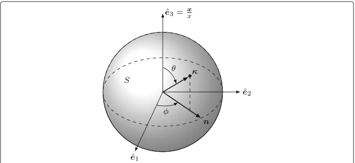
Away from the origin, we can choose the hemisphere having the directionx as the zenith. This is a convenient choice because all points κ on such a hemisphere satisfy the conditionκ·x≥0. This hemisphere can be parameterized by the zenith angleθand the azimuth angleφ, as shown in Fig.1. In this reference system, the unit vectorκcan be expressed as

Fig. 1The unit sphere in Fourier space. The unit vectorκ(θ,φ)is defined by the azimuth angleφ, and the zenith angleθmeasured from the axiseˆ3=x/x

wheree3ˆ =x/x. Finally, lettingq=cosθ, the elementary solid angle becomes

dω=sinθdθdφ= −dqdφ, (35)

and

κ(q,φ)=

1−q2_{cosφe1ˆ +}

1−q2_{sinφˆe2+qe3ˆ . (36)}

Therefore the Green tensor of the anisotropic Mindlin differential operator of first order finally becomes

G(x)= 1 8π2

2π

0

1

0 C −1

2(κ)_exp−_qx−1(κ) −1(κ)C−12(κ)_dqdφ_{. (37)}

The first two gradients of the Green tensor

The first two gradients of the Green tensor are computed directly by differentiation of (32). The first gradient reads

∇G(x)= − 1 16π2

SC

−1

2(κ)_exp−|κ·_x|−1(κ) −2(κ)

×C−12(κ)⊗κ_sign(κ·_x)_dω_{. (38)}

In components this is:

Gij,m(x)= −

1 16π2

S

C−12(κ)_exp−|κ·_x|−1(κ) −2(κ)

×C−12(κ)

ijκmsign(κ·x)dω. (39)

con-venient to express this result in reference system of Fig.1. Doing so we find the alternative representation

Gij,m(x)= −

1 8π2

2π

0

1

0

C−12(κ)_exp−|κ·_x|−1(κ) −2(κ)

×C−12(κ)

ijκmdq dφ. (40)

The second gradient of the Green tensor reads

∇∇G(x)= 1 16π2

S

C−1

2(κ)_exp−|κ·_x|−1(κ)

×−3_(κ)C−1

2(κ)⊗κ⊗κ

−C−1

2(κ)−2(κ)C−21(κ)⊗κ⊗κδ(κ·_x)

dω. (41)

Lettingn(φ)= κ(π/2,φ)be a unit vector on the equatorial planeκ·x= 0, we finally obtain

∇∇G(x)= 1 16π2

SC

−1

2(κ)exp−|κ·_x|−1(κ)

×−3_(κ)C−1

2(κ)⊗κ⊗κ_dω

− 1 8π2_x

2π

0

C−1

2(_n)−2(_n)C−12(_n)⊗_n⊗_ndφ_{. (42)}

Note that the second gradient of the Green tensor is singular at the origin.

The classical limit

It is now shown that Green tensor (32) converges to the classical Green tensorG0(Lifshitz and Rosenzweig1947; Synge1957) when the field pointxis sufficiently far from the origin compared to the characteristic length scales, that is when

|κ·x|/λi1, (43)

whereλiis an eigenvalue of, andi=1, 2, 3. This important property guarantees that the

non-singular Green tensor (37) regularizes the classical anisotropic Green tensor in the far field. Moreover, as a special case satisfying condition (43), the classical Green tensor G0is also recovered in the limit of vanishing tensor of strain gradient coefficientsD. The classical Green tensorG0is readily recovered if we consider the limit5

lim |κ·x|/λi→∞

exp−|κ·x|−1(κ) −1(κ)= 2I

x δ(κ· ˆx), (44)

wherexˆ=x/xandIis the identity tensor. In fact, the substitution of (44) into (32) yields

G(x)→G0(x)= 1 8π2_x

SC

−1_{(κ) δ(κ·x)dω=} 1 8π2_x

2π

0 C

−1_{(n)dφ. (45)}

Special cases

In this section we show that the Green tensor (32) generalizes other results obtained in the literature.

The weakly non-local Green tensorGNL

Lazar and Po (2015b) have considered a simplified strain gradient elasticity theory under the assumption

Dijmkln=CijklLmn, (46)

a framework which was named Mindlin’s strain gradient elasticity with weak non-locality because of its relation to non-local theories (Lazar, M et al.: Nonlocal anisotropic elasticity: fundamentals and application to three-dimensional dislocation problems, sub-mitted for publication) (Lazar and Agiasofitou2011). The Green tensor (32) recovers our previous result as a special case. In fact, under the previous assumption, we have

(κ)=IκT_{Lκ, (47)}

and

exp−|κ·x|−1(κ) −1(κ)=I exp

−_√|κ·x| κT_Lκ

√

κT_Lκ .

Therefore the Green tensor becomes

GNL(R)= 1 16π2

SC

−1_(κ)exp

−_√|κ·x| κT_Lκ

√

κT_Lκ dω, (48)

which is the expression given in Lazar and Po (2015b).

The Green tensor of anisotropic gradient elasticity of Helmholtz typeGH

An even simpler theory, named Mindlin’s gradient elasticity of Helmholtz type, has been proposed by Lazar and Po (2015a). The theory is characterized by only one gradient length scale parameter, which renders the tensorLdiagonal:

L=2I. (49)

The non-singular Green tensor of this theory is obtained by substituting (49) in (48), thus yielding

GH(R)= 1 16π2

SC

−1_(κ)exp

−|κ·x|

dω, (50)

which coincides with the expression given in Lazar and Po (2015a).

The isotropic Green tensorGI

Cijkl =λδijδkl+μ

δikδjl+δilδjk

, (51)

whereλandμare the Lamé constants. On the other hand, the isotropic tensorDreads

Dijmkln=

a1 2

δijδkmδln+δijδknδlm+δklδimδjn+δklδinδjm

+ a3 2

δjkδimδkl+δikδjmδnl+δilδjmδkn+δjlδimδkn

+ a5 2

δjkδinδlm+δikδjnδlm+δjlδkmδin+δilδkmδjn

+2a2δijδklδmn+a4

δilδjkδmn+δikδjlδmn

, (52)

wherea1,a2,a3,a4,a5are the gradient parameters in isotropic Mindlin’s first strain gra-dient elasticity theory (Mindlin1964) (see also Mindlin (1968b), Lazar and Po (2016)). Therefore, the matricesC(κ)andD(κ)become, respectively

Cik(κ)=(λ+2μ)κiκk+μ

δik−κiκk

, (53)

Dik(κ)=2(a1+a2+a3+a4+a5)κiκk

+ 1

2(a3+2a4+a5)

δik−κiκk

=(λ+2μ) 2₁κiκk+μ 22

δik−κiκk

. (54)

The two characteristic lengths1and2introduced above are defined as

2 1=

2(a1+a2+a3+a4+a5)

λ+2μ , (55)

2 2=

a3+2a4+a5

2μ . (56)

Owing to the special structure6 of C(κ) and D(κ), the following results are easily obtained:

C−12

ij (κ)=

1

√_μδij−κiκj

− √ 1

λ+2μκiκj (57)

−1

ij (κ)=

1

2

δij−κiκj

+ 1

1κiκj

. (58)

The matrix−1 admits the eigenvalue 1/1, corresponding to the eigenvector v1ˆ = κ. The degenerate eigenvalue 1/2has multiplicity two, corresponding to two arbitrary eigenvectorsv2ˆ andv3ˆ perpendicular toκ. Choosing such eigenvectors to be mutually orthogonal, the matrix−1admits the eigen decomposition−1=QD−1QT. Here

Q=[v1ˆ v2ˆ v3ˆ ] (59)

is an orthogonal matrix whose columns are the eigenvectors of−1, and

D−1=diag

1

1 , 1

2 , 1

2

(60)

C−1

2_Q=_Qdiag

−√_λ+1 2μ,

1 √_μ, _√1

μ

. (61)

Using these results in (32), we obtain

GI(x)= 1 16π2

SC

−1

2_Qexp−|κ·_x|_D−1 _D−1_QTC−12_dω

= 1 16π2

SQdiag ⎧ ⎨ ⎩

e−|κ₁·x| 1(λ+2μ)

, e −|κ·x|

₂

2μ , e

−|κ·x|

₂

2μ ⎫ ⎬ ⎭QTdω

= 1 16π2

S

e−|κ₁·x| (λ+2μ)1ˆ

v1⊗ ˆv1dω

+ 1 16π2

S

e−|κ2·x|

μ2

ˆ

v2⊗ ˆv2+ ˆv3⊗ ˆv3

dω. (62)

Because they form an orthonormal basis, the three eigenvectors satisfy the identityv1ˆ ⊗

ˆ

v1+ ˆv2⊗ ˆv2+ ˆv3⊗ ˆv3=I, hence we have

GI(x)= 1 16π2

S ⎡

⎣ e

−|κ·x|

1

(λ+2μ)1κ⊗κ+

e−|κ2·x|

μ2 (

I−κ⊗κ) ⎤

⎦dω. (63)

The integral over the unit sphere is carried out using the relation

S

e−|κ·x|

κiκjdω=2π ∂i∂jA(x,), (64)

where the scalar functionA(x,)is

A(x,)=x+ 2

2

x −

22

x e

−x/_{. (65)}

The scalar functionA(x,)can be regarded as a regularized distance function in the sense thatA(x,)tends toxwhenx/1, while it smoothly approaches 2for smallx, as shown in Fig.2. By sake of (64), the Green tensor finally becomes:

Gij(x)=

1 8πμ

_μ

λ+2μ∂i∂jA(x,1)+

δij−∂i∂j

A(x,2)

. (66)

This result can also be obtained by direct inverse Fourier transform of (23), as shown in Appendix1. A more detailed analysis of the isotropic Green tensor (66) can be found in Lazar and Po (2018).

A comparison with molecular statics: The Kelvin problem

Fig. 2Plot of the regularized distance functionA(x,)

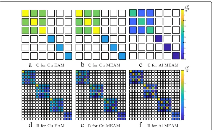
We choose face-centered-cubic Aluminum and Copper for this comparison, and con-sider the following two interatomic potentials: the modified-embedded-atom-method (MEAM) by Lee et al. (2001), and the embedded-atom-potential by Mendelev et al. (2008), which are archived in the OpenKIM repository. Elastic and gradient-elastic con-stants for these potentials were computed using the method described in Admal et al. (2016), and they are available on the KIM repository (Lee2014; Mendelev2014). For con-venience, the values of the independent elastic and gradient-elastic constants are reported in Table1. These components are used to populate the elastic tensorsCandD(Admal et al.2016; Auffray et al.2013). The Voigt structure of the resulting tensorsCandDis shown in Fig.3.

The atomistic system is constructed by stacking together 15×15×15 unit cells resulting in 13500 atoms. A force of 0.0116 eV/Å in thex1 direction is imposed on the central

Table 1Elastic and gradient-elastic constants obtained from the interatomic potentials Lee (2014) and Mendelev (2014)

Cu EAM Cu MEAM Al MEAM

C1,1[ eV/Å3] 1.0868 1.0994 7.1366·10−1 C1,2[ eV/Å3] 7.9386·10−1 7.7973·10−1 3.8649·10−1 C4,4[ eV/Å3] 5.2252·10−1 5.1043·10−1 1.9704·10−1

a

b

c

d

e

f

Fig. 3Voigt representation of the elastic tensorsCand gradient-elastic tensorDfor fcc Al and Cu, computed from the interatomic potentials Lee (2014) and Mendelev (2014).aanddCu for EAM potential (Mendelev

2014).bandeCu for MEAM potential (Lee2014).candfAl for MEAM potential (Lee2014)

atom of the system, and displacement boundary conditions are imposed on five layers of atoms close to the boundary using the classical solution given in Eq. (45). The padding atoms thickness is 0.15 times the size of the box. A MS simulation is carried out using the above-mentioned boundary conditions resulting in a deformed crystal. The resulting displacement field normalized with respect to the force on the central atom yields the atomistic Green tensor component fields.

Simulation results are shown in Fig.4, where we compare the Green tensor compo-nents G11(x1, 0, 0) andG22(x1, 0, 0). Despite the fact that these potentials were never fitted to gradient-elastic constants, it can be observed that the analytical predictions are in good agreement with MS calculations, with a maximum error at the origin in the order of 5-30%, depending on the potential used. It should be noted that, compared to the EAM potential, the MEAM potential better compares to the analytical results, pos-sibly as a result of artifacts in gradient-elastic constants evaluated by EAM potentials (Admal et al.2016).

Summary and conclusions

a

b

c

d

e

f

Fig. 4Components of the Green tensor for fcc Al and Cu, and comparison to atomistic calculations obtained from the interatomic potentials Lee (2014) and Mendelev (2014).a-bCu for EAM potential (Mendelev2014). c-eCu for MEAM potential (Lee2014).e-fAl for MEAM potential (Lee2014)

Endnotes

1_{The inelastic distortion comprises plastic effects, and is typically an incompatible field.}

When the inelastic distortion is absent the elastic distortion is compatible.

2_{Due to the centrosymmetry, there is no coupling betweene}

ijand∂mekl.

3_{The Fourier transform and its inverse are defined as, respectively (Vladimirov1971):}

ˆ

f(k)=

R3f(x)e

−ik·x_{dV, (67)}

f(x)= 1 (2π)3

R3 ˆ

f(k)eik·xdVˆ . (68) For a real-valued function, the inverse Fourier transform is

f(x)= 1 (2π)3

R3 ˆ

f(k) cos(k·x)dVˆ . (69)

4_{The proof of (31) descends from the fact that}2_{(κ)is a real SPD matrix, and therefore}

it admits the eigen-decomposition

2_(κ)=Q(κ)D2_(κ)QT_{(κ), (70)}

where D2(κ) = diagλ2_i(κ) is the diagonal matrix of the positive eigenvalues of 2_{(κ), andQ(κ)is the orthogonal matrix of its eigenvectors. With this observation, we} immediately obtain

_∞

0

I+k22(κ)−1 cos(kκ·x)dk=

_∞

0

Q(κ)I+k2D2(κ)QT(κ)−1cos(kκ·x)dk

=Q(κ)

_∞

0 diag

cos(kκ·x) 1+k2_λ2

i(κ)

dkQT(κ). With the help of the definite integral 3.767 in Gradshteyn and Ryzhik (2007), we obtain

_∞

0

I+k22(κ)−1cos(kκ·x)dk= π

2 Q(κ)diag

e−|κ·x|/λi(κ)

λi(κ)

QT(κ)

= π

2 Q(κ)diag

e−|κ·x|/λi(κ) _D−1(κ)_QT(κ)

= π

2 Q(κ) exp

−|κ·x|D−1(κ) QT(κ)−1(κ)

= π 2 exp

−|κ·x|−1(κ) −1(κ).

In the last step we have used the property that the matrix exponential is an isotropic tensor-valued function of its argument.

5_{Using the eigen-decomposition (70):}

lim |κ·x|/λi→∞

exp−|κ·x|−1(κ) −1(κ)

= lim |κ·x|/λi→∞

Q(κ)exp−|κ·x|D−1(κ) D−1(κ)QT(κ)

= lim |κ·x|/λi→∞

Q(κ)diag

exp{−|κ·x|/λi(κ)} λi(κ)

QT(κ)

=Q(κ)2I

x δ(κ· ˆx)Q

T_(κ)= 2I

x δ(κ· ˆx).

6_{Consider a matrixAwith structure}

Ifa>b>0, then the matrix is SPD, and a unique SPD square root ofAijexists with form A 1 2 ij = √

aκiκj+

√

b(δij+κiκj). (72)

Moreover, the inverse ofAijreads

A−_ij1= 1 aκiκj+

1

b(δij−κiκj). (73)

Appendix 1: Direct derivation of Mindlin’s isotropic strain gradient elasticity of form II

Plugging (53) and (54) into (23) we have

G(k)=

(λ+2μ)1+k22₁κ⊗κ+μ1+k22₂(I−κ⊗κ)−1

k2 . (74)

Owing to its special structure (see footnote6), the matrix in the numerator can be easily inverted. In index notation the result is

Gij(k)= κiκj

(λ+2μ)k2_1+k22 1

+ δij−κiκj

μk2_1+k22 1

= kikj

(λ+2μ)k4_1+k22 1

+ k2δij−kikj

μk4_1+k22 1

. (75)

Using the general form of the Fourier transform of the derivative, the Green tensor in real space is obtained as

Gij(x)= −_λ∂₊i∂j

2μF −1

! 1

k4_1+k22 1

"

−δij_μ−∂i∂jF−1 !

1

k4_1+k22 1

" . (76)

Now consider the identity

F−1 !

1

k4_1+k22 "

=F−1 !

1

k4− 2

k2 + 4 1+k22

1 "

= − 1 8π

x+ 2

2

x −

22

x e

−x/

= − 1

8πA(x,). (77)

Using (77) in (76), the Green tensor (66) is readily recovered.

Abbreviations

API: Application programming interface; EAM: Embedded atom method; KIM: Open Knowledgebase of interatomic models; MEAM: Modified embedded atom method; PDE: Partial differential equation; SPD: Symmetric positive definite

Funding

G.P. acknowledges the support of the U.S. Department of Energy, Office of Fusion Energy, through the DOE award number DE-SC0018410, the Air Force Office of Scientific Research (AFOSR), through award number FA9550-16-1-0444, and the National Science Foundation, Division of Civil, Mechanical and Manufacturing Innovation (CMMI), through award number 1563427 with UCLA. N.A. acknowledges the support of the US Department of Energy’s Office of Fusion Energy Sciences, Grant No. DE-SC0012774:0001. M.L. gratefully acknowledges a grant from the Deutsche

Forschungsgemeinschaft (Grant No. La1974/4-1).

Availability of data and materials

Elastic and gradient-elastic material constants used to obtain the results in “A comparison with Molecular Statics: The Kelvin problem” section are freely available as part of the Open Knowledgebase of Interatomic Models (KIM).

Authors’ contributions

G.P. and M.L. obtained the expression of the Green Tensor. N.A. and G.P. carried out the numerical analysis. All authors read and approved the final manuscript.

Competing interests

Publisher’s Note

Springer Nature remains neutral with regard to jurisdictional claims in published maps and institutional affiliations.

Author details

1_{Department of Mechanical and Aerospace Engineering, University of California Los Angeles, Los Angeles 90095, CA,} USA.2_{Department of Mechanical and Aerospace Engineering, University of Miami, Coral Gables 33146, FL, USA.} 3_{Department of Materials Science and Engineering, University of California Los Angeles, Los Angeles 90095, CA, USA.} 4_{Department of Physics, Darmstadt University of Technology, Hochschulstr. 6, 64289 Darmstadt, Germany.}5_Department of Mechanical Science and Engineering University of Illinois Urbana–Champaign, Illinois, USA.

Received: 15 November 2018 Accepted: 18 February 2019

References

N. C. Admal, J. Marian, G. Po, The atomistic representation of first strain gradient elastic tensors. J. Mech. Phys. Solids.99, 93–115 (2016)

H. Askes, E. C. Aifantis, Gradient elasticity in statics and dynamics: an overview of formul‘ations, length scale identification procedures, finite element implementations and new results. Int. J. Solids Struct.48(13), 1962–1990 (2011) N. Auffray, H. Le Quang, Q. C. He, Matrix representations for 3D strain gradient elasticity. J. Mech. Phys. Solids.61,

1202–1223 (2013)

D. J. Bacon, D. M. Barnett, R. O. Scattergood, Anisotropic continuum theory of defects. Prog. Mater. Sci.23, 51–262 (1979) D. M. Barnett, The precise evaluation of derivatives of the anisotropic elastic Green functions. Phys. Stat. Sol. (B).49,

741–748 (1972)

A. A. Becker,The Boundary Element Method in Engineering: A Complete Course. (Mcgraw-Hill, 1992)

A. C. Eringen,Microcontinuum field theories: I. Foundations and solids. (Springer Science & Business Media, 1999) A. C. Eringen,Nonlocal continuum field theories. (Springer Science & Business Media, 2002)

I. S. Gradshteyn, I. M. Ryzhik,Table of Integrals, Series, and Products, 7th ed. (Academic Press, 2007)

G. Green,An Essay on the Application of Mathematical Analysis to the Theories of Electricity and Magnetism. (Nottingham (the author), 1828)

L. Kelvin,Mathematical and Physical Papers, Vol. 1. (Cambridge University Press, Cambridge, 1882), p. 97 E. Kröner, On the physical reality of torque stresses in continuum mechanics. Int. J. Engng. Sci.1, 261–278 (1963) M. Lazar, Irreducible decomposition of strain gradient tensor in isotropic strain gradient elasticity. Z. Angew. Math. Mech.

96, 1291–1305 (2016)

M. Lazar, E. Agiasofitou, Screw dislocation in nonlocal anisotropic elasticity. Int. J. Eng. Sci.49, 1404–1414 (2011) M. Lazar, G. Po, On Mindlin’s isotropic strain gradient elasticity: Green tensors, regularization, and operator-split. J.

Micromech. Mol. Phys., 1840008 (2018)

M. Lazar, G. Po, The non-singular Green tensor of gradient anisotropic elasticity of Helmholtz type. Eur. J. Mech. A Solids. 50, 152–162 (2015a)

M. Lazar, G. Po, The non-singular Green tensor of Mindlin’s anisotropic gradient elasticity with separable weak non-locality. Phys. Lett. A.379, 1538–1543 (2015b)

B.-J. Lee, Second nearest-neighbor modified embedded-atom-method (2NN MEAM) (2014).https://openkim.org/cite/ MD_111291751625_001

B.-J. Lee, M. I. Baskes, H. Kim, Y. Koo Cho, Second nearest-neighbor modified embedded atom method potentials for bcc transition metals. Phys. Rev. B.64, 184102 (2001)

I. M. Lifshitz, L. N. Rosenzweig, On the construction of the Green tensor for the basic equation of the theory of elasticity of an anisotropic medium. Zh. Eksper. Teor. Fiz.17, 783–791 (1947)

M. I. Mendelev, M. J. Kramer, C. A. Becker, M. Asta, Analysis of semi-empirical interatomic potentials appropriate for simulation of crystalline and liquid Al and Cu. Phil. Mag.88, 1723–1750 (2008)

M. I. Mendelev, FS potential for Al (2014).https://openkim.org/cite/MO_106969701023_001 R. D. Mindlin, Micro-structure in linear elasticity. Arch. Rational. Mech. Anal.16, 51–78 (1964)

R. D. Mindlin, N. N. Eshel, On first strain gradient theories in linear elasticity. Int. J. Solids Struct.4, 109–124 (1968a) R. D. Mindlin, inMechanics of Generalized Continua, IUTAM Symposium. ed. by E. Kröner, Theories of elastic continua and

crystal lattice theories (Springer, Berlin, 1968b), pp. 312–320

R. D. Mindlin, Elasticity, piezoelectricity and crystal lattice dynamics. J. Elast.2, 217–282 (1972) T. Mura,Micromechanics of Defects in Solids, 2nd edn, (Martinus Nijhoff, Dordrecht, 1987)

C. Polizzotto, Anisotropy in strain gradient elasticity: Simplified models with different forms of internal length and moduli tensors. Eur. J. Mech.-A/Solids.71, 51–63 (2018)

D. Rogula, Some basic solutions in strain gradient elasticity theory of an arbitrary order. Arch. Mech.25, 43–68 (1973) E. B. Tadmor, R. S. Elliott, J. P. Sethna, R. E. Miller, C. A. Becker, The potential of atomistic simulations and the

Knowledgebase of Interatomic Models. JOM.63, 17–17 (2011)

E. B. Tadmor, R. S. Elliott, S. R. Phillpot, S. B. Sinnott, NSF cyberinfrastructures: a new paradigm for advancing materials simulation. Curr. Opin. Solid State Mater. Sci.17(6), 298–304 (2013)

E. B. Tadmor, R. E. Miller,Modeling materials: continuum, atomistic and multiscale techniques. (Cambridge University Press, 2011)

J. L. Synge,The Hypercircle in Mathematical Physics. (Cambridge University Press, Cambridge, 1957) C. Teodosiu,Elastic Models of Crystal Defects. (Springer, Berlin, 1982)

D. R. Trinkle, Lattice Green function for extended defect calculations: Computation and error estimation with long-range forces. Phys. Rev. B.78, 014110 (2008)