Monolithic and partitioned Rosenbrock-based time integration methods for dynamic substructure tests

(1)

University of Trento University of Brescia University of Padova University of Trieste University of Udine University IUAV of Venezia

Jia Chuanguo (Ph.D. Student)

MONOLITHIC AND PARTITIONED

ROSENBROCK-BASED TIME INTEGRATION METHODS FOR

DYNAMIC SUBSTRUCTURE TESTS

Prof. Oreste S. Bursi (Tutor)

(2)

UNIVERSITY OF TRENTO

Structural Engineering - Modelling, Preservation and Control of Materials and Structures

Cycle: XXII

Head of the Doctoral School: Prof. Davide Bigoni

Final Examination 19 / 04 / 2010

Board of Examiners

Prof. Mauro Da Lio (Università di Trento)

Prof. Alain Molinari (Università Paul Verlaine-Metz)

(3)

SUMMARY

Real-time testing with dynamic substructuring provides an efficient way to simulate the nonlinear dynamic behaviour of civil structures or mechanical facilities. In this technique, the test structure is divided onto two substructures: the relatively crucial substructure is tested physically and the other is modelled numerically in the computer. The key challenge is to ensure that both substructures interact in real-time, in order to simulate the behaviour of the emulated structure. This has special demands on the utilized integration methods and their implementations. Researchers have devoted significant effort to implement second-order integrators, such as Newmark integration methods, in a monolithic way where both substructures are integrated altogether. However, in view of large and complex structures, time integration methods are required to advance large-scale systems hence endowed with high-frequency components of the response or mixed first- and second- order systems like in the case of controlled systems. In this case, the monolithic implementation of a second-order time integration method becomes inefficient or inaccurate.

With these promises, the thesis adopts the Rosenbrock-based time integration methods for both dynamic simulations of complex systems and substructure tests, and in particular, focuses on the development of monolithic schemes with subcycling strategies for nonlinear cases and partitioned methods with staggered and parallel solution procedures for linear and nonlinear cases.

(4)

(5)

(6)

ACKNOWLEDGEMENTS

First of all, I want to express my gratitude to my supervisor Prof. Oreste S. Bursi for his constant encouragement and illuminating instruction in all the time of the research. I am heartily thankful to him for all his help in my life.

I would like to thank Dr. Alessio Bonelli, Dr. Leonardo Vulcan and Dr. Leqia He who helped me a lot on time integration methods and gave me valuable advice. I also

owe my sincere gratitude to Alessandro Zambonin for his contribution to the partitioned time integration methods. Moreover, I want to thank Iker.Elorza and Wang Zhen for collaborating in design the TT1 test-rig.

I want to thank the University of Trento for giving me the Ph.D. fellowship to commence this thesis and to do the necessary research work. Meanwhile, the research has benefited from the financial support of the SERIES project.

I have also enjoyed a lot of support from many people around me. For this I think the entire DIMS group of the UNITN. I owe special thanks to all of my colleagues along the way: Dr. Marco Molinari, Dr. Fabio Ferrario, Li Gu, Alireza Savadkoohi, Seema, Wu Huayong, Nicola Tondini, Md Shahin Reza and Yue Yanchao.

(7)

C

ONTENTS

1 Introduction 1

1.1 Context . . . 1

1.2 Motivation of the research . . . 3

1.3 Thesis organization . . . 7

2 State of the art 11 2.1 Introduction . . . 11

2.2 Experimental dynamic tests . . . 11

2.2.1 Quasi-static testing method . . . 12

2.2.2 Shaking table testing method . . . 12

2.2.3 Pseudo-dynamic testing method . . . 13

2.2.4 PsD testing method with dynamic substructuring . . . 15

2.2.5 Real-time testing with dynamic substructuring . . . 16

2.3 Integration methods for RTDS testing . . . 18

2.3.1 Central difference method . . . 20

2.3.2 Explicit Newmark method . . . 21

2.3.3 Constant average acceleration method . . . 23

2.3.4 Generalized-αmethod . . . 24

2.3.5 Newmark-Chang method . . . 25

2.3.6 The CR method . . . 26

2.3.7 Summary . . . 27

2.4 Partitioned time integration methods . . . 27

2.4.1 Introduction to domain decomposition methods . . . 28

(8)

2.4.3 Introduction to the GC method . . . 32

2.4.4 The interfield parallel method - the PM method . . . 35

2.5 Summary . . . 38

3 Analysis of L-stable real time compatible algorithms 39 3.1 Introduction . . . 39

3.2 Rosenbrock based algorithms . . . 40

3.2.1 L-stable real-time one-stage (LSRT1) method . . . 41

3.2.2 L-stable real-time two-stage (LSRT2) method . . . 42

3.2.3 L-stable real-time three-stage (LSRT3) method . . . 42

3.3 Accuracy analysis . . . 43

3.3.1 Local truncation error analysis for the LSRT1 algorithm . . . . 44

3.3.2 Local truncation error analysis for the LSRT2 algorithm . . . . 45

3.3.3 Global error analysis for the LSRT algorithm . . . 46

3.4 Stability analysis via the energy method . . . 47

3.4.1 Stability analysis for the LSRT1 algorithm . . . 48

3.4.2 Stability analysis for the LSRT2 algorithm . . . 49

3.5 Numerical experiments on a spring-pendulum oscillator . . . 52

3.5.1 Governing equations . . . 53

3.5.2 Static analysis . . . 55

3.5.3 Numerical integration . . . 58

3.5.3.1 Implementation . . . 59

3.5.3.2 Absolute stability analysis . . . 60

3.5.3.3 Accuracy analysis . . . 61

3.5.3.4 Numerical simulation . . . 63

3.6 Conclusions . . . 63

4 Monolithic time integration methods for real-time substructure tests 65 4.1 Introduction . . . 65

4.2 Substructuring strategy . . . 68

4.2.1 Partitioning and coupling . . . 68

(9)

4.3.1 Subcycling strategies for the LSRT algorithms . . . 71

4.3.2 Subcycling strategies for the Explicit Newmark method and the Newmark-Chang method . . . 73

4.4 Numerical application on a coupled spring-pendulum system . . . 74

4.4.1 Zero Stability analysis . . . 74

4.4.2 Numerical simulations . . . 76

4.4.3 Accuracy analysis . . . 77

4.5 Application tests . . . 80

4.5.1 The Bouc-Wen model . . . 80

4.5.2 Heterogeneous tests . . . 81

5 Partitioned time integration methods based on acceleration continuity 87 5.1 Introduction . . . 87

5.2 Derivation of an explicit Lagrange multiplier . . . 89

5.3 Formulations of the partitioned time integration methods . . . 92

5.3.1 A parallel solution procedure with no subcycling and based on the LSRT1 integrator (APNR1) . . . 93

5.3.2 A parallel solution procedure with no subcycling and based on the LSRT2 integrator (APNR2) . . . 94

5.4.1 Local truncation error analysis of theAPNR1method . . . 97

5.4.2 Local truncation error analysis of theAPNR2method . . . 98

5.4.3 Global error estimates . . . 100

5.5 Stability analysis . . . 100

5.5.1 Stability analysis for theAPNR1method . . . 101

5.5.2 Stability analysis for theAPNR2method . . . 102

6 Partitioned time integration methods with a staggered solution proce-dure 107 6.1 Introduction . . . 107

(10)

6.2.1 A staggered solution procedure with subcycling and based on

the LSRT1 integrator (ASSR1) . . . 109

6.2.2 A staggered solution procedure with subcycling and based on the LSRT2 integrator (ASSR2) . . . 110

6.3.1 Local truncation error analysis of theASSR1method . . . 114

6.3.2 Local truncation error analysis of theASSR2method . . . 115

6.3.3 Local truncation error analysis for the GC method . . . 120

6.4 Numerical analysis and simulations of a Single-DoF split mass system 123 6.4.1 The Single-DoF split mass system . . . 123

6.4.2 Spectral stability analysis . . . 124

6.4.3 Investigation of the principal eigenvalues . . . 135

6.4.4 Investigation of spurious eigenvalues . . . 136

6.4.5 Numerical convergence analysis . . . 140

6.5 Numerical simulation of partitioned Multiple-DoF linear systems . . . . 144

6.5.1 Partitioned Multiple-DoF systems . . . 144

6.5.2 Spectral stability analysis for the Multiple-DoF systems . . . . 146

6.5.3 Drift analysis . . . 149

6.5.4 Simulations . . . 153

7 Partitioned time integration methods with an interfield parallel solution procedure 159 7.1 Introduction . . . 159

7.2 Formulations of parallel partitioned methods . . . 160

7.2.1 An interfield parallel solution procedure based on the LSRT1 time-stepping method (APSR1) . . . 160

7.2.2 An interfield parallel solution procedure based on the LSRT2 time-stepping method (APSR2) . . . 162

(11)

7.4.3 Numerical simulation . . . 174

7.5 Numerical analysis and simulations for Multiple-DoF split mass systems179 7.5.1 Spectral stability analysis . . . 179

8 Partitioned time integration methods based on projection methods 187 8.1 Introduction . . . 187

8.2 Formulation of the projection methods . . . 188

8.2.1 Derivation of the LSRT1-based projection method (VPNR1) . . 188

8.2.2 Derivation of the LSRT2-based projection method (VPNR2) . . 189

8.3.1 Local truncation error analysis for the LSRT1-based projection method . . . 190

8.3.2 Local truncation error analysis for the LSRT2-based projection method . . . 193

8.4 Stability analysis . . . 197

8.5 Numerical analysis and simulations of a Single-DoF split mass system 202 8.5.1 Spectral stability analysis . . . 202

8.6 Numerical simulation of Multiple-DoF systems . . . 213

9 Experimental validation and real-time implementation 221 9.1 Introduction . . . 221

9.2 General test rig design . . . 221

9.3 Detailed experimental equipment . . . 223

9.3.1 The masses and the bearings . . . 225

9.3.2 Springs and damping devices . . . 227

9.3.3 Electro-thrust actuators . . . 228

(12)

9.3.5 Instrumentation package . . . 230

9.4 Different test configurations . . . 231

10 Conclusions and future perspectives 235

10.1 Summary . . . 235

(13)

L

IST OF

F

IGURES

1.1 Block diagram representation including delay for RTDS tests . . . 5

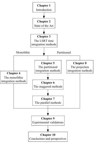
1.2 Organization of the thesis . . . 8

2.1 Flow of the PsD testing method . . . 14

2.2 Control loop of the RTDS testing method . . . 17

2.3 (a) Overlapping domain decomposition method; (b) Non-overlapping domain decomposition method . . . 28

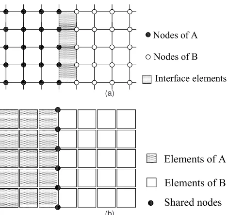
2.4 The partitioning approach: (a) Node partitioning; (b) element partitioning 29 2.5 The solution procedure of the GC method . . . 32

2.6 The solution procedure of the PM method . . . 35

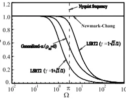
3.1 Spectral radiiρof the LSRT2 method with respect to the Generalized-αmethod and Newmark-Chang method vs. the non-dimensional fre-quencyΩ . . . 42

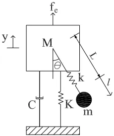
3.2 Schematic representation of a spring-pendulum system . . . 53

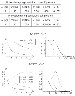
3.3 Spectral radii of the LSRT methods applied to the uncoupled spring-pendulum oscillator linearized aroundθ= 0: a) the LSRT2 method; b) the LSRT3 method. . . 61

(14)

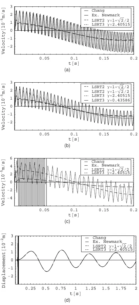
3.5 Numerical simulations for the uncoupled spring-pendulum stiff problem

summarized in Table 3.1: (a) velocity ˙l obtained with different methods

and∆t0 = 1/3ms; (b) velocity ˙l provided by different LSRT algorithms and∆t0= 1/3ms; (c) velocity ˙l with∆t0= 2ms; (d) displacement y with ∆t0= 2ms. . . 64

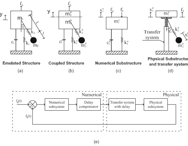
4.1 (a)-(d) Schematic representation of a substructured spring-pendulum

oscillator; (e) block diagram representation including delay . . . 69

4.2 Coupled integration in real time: (a) force-displacement(mixed)

cou-pling strategy; and (b) mixed strategy with algebraic coucou-pling conditions 70

4.3 Solution sequence of the time integration of a coupled system with

the LSRT3 algorithm: (a) single step strategy; (b) multiple step strategy with equilibrium-based interpolation; (c) multiple

time-step strategy with differentiation-based interpolation. . . 72

4.4 Numerical simulations for the coupled spring-pendulum stiff problem

summarized in Table 3.1: (a) velocity ˙x2p obtained with different meth-ods and∆t0= 1/3ms; (b) velocity ˙x2pprovided by different LSRT algo-rithms and ∆t0 = 1/3ms; (c) velocity ˙x₂p with∆t0 = 2ms; (d) displace-ment x₁pwith∆t0= 2ms. . . 78

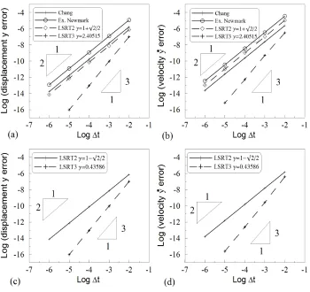
4.5 Convergence of displacement and velocity for the coupled spring-pendulum

nonstiff problem summarized in Table 3.1: (a) displacement x1 error without subcycling; (b) velocity ˙x1error without subcycling; (c)

displace-ment x2error with equilibrium-based interpolation; (d) displacement x2

error with differentiation-based interpolation. . . 79

4.6 Real-time test on an SDoF system with a nonlinear NS excited by an external sinusoidal force with f = 1.5 Hz and A = 12 N: (a) PS and

set-up; (b) experimental results. . . 82

4.7 Real-time test on a spring-pendulum system with a linear NS excited

by an external sinusoidal force with f = 2.2 Hz and A = 12 N: (a) PS

and set-up; (b) experimental results. . . 83

4.8 Real-time test on a spring-pendulum system with nonlinear Numerical

Substructure excited by an external sinusoidal force with f = 1.2 Hz and

(15)

5.1 The staggered solution procedure of the LSRT1-based partitioned method

with ss = 1 . . . 93

with ss = 1 . . . 95

with ss>1 . . . 111

with ss>1 . . . 113

6.3 Representation of the linear interpolation in the GC method and its equivalent solution procedure . . . 122

6.4 A Single-DoF split mass system . . . 124

6.5 |λi |for the partitioned method integrated with LSRT1 and ss = 1: (a)

b1= 2and (b) b1= 10. . . 126

b1= 0.1, (b) b1= 1, (c) b1= 2, and (d) b1= 10 . . . 127

6.8 | λi | for the partitioned method integrated by LSRT2 with γA = γB =

1−√2

2 and ss = 1: (a) b1= 2and (b) b1= 10 . . . 127 6.9 | λi | for the partitioned method integrated by LSRT2 with γA = γB =

1 +√2

2 and ss = 1: (a) b1= 2and (b) b1= 10 . . . 127 6.10| λi | for the partitioned method integrated by LSRT2 with γA = 1−

√ 2

2 ,γB = 1 + √

2

2 and ss = 1: (a) b1= 2and (b) b1= 10 . . . 128 6.11| λi | for the partitioned method integrated by LSRT2 withγA = 1 +

√ 2

2 ,γB = 1− √

2

2 and ss = 1: (a) b1= 2and (b) b1= 10 . . . 128 6.12| λi | for the partitioned method integrated by LSRT2 with γA = γB =

1−√2

1 + √

2

2 and ss = 2: (a) b1= 2and (b) b1= 10 . . . 129 6.14| λi | for the partitioned method integrated by LSRT2 with γA = 1−

√ 2

2 ,γB = 1 + √

2

(16)

6.15| λi | for the partitioned method integrated by LSRT2 with γA = 1 +

√ 2

2 ,γB = 1− √

2

1−√2

2 and ss = 10: (a) b1= 0.1, (b) b1= 1, (c) b1= 2, and (d) b1= 10 . 130 6.17| λi | for the partitioned method integrated by LSRT2 with γA = γB =

1 + √

2

2 and ss = 10: (a) b1= 0.1, (b) b1= 1, (c) b1= 2, and (d) b1= 10 . 130 6.18| λi | for the partitioned method integrated by LSRT2 with γA = 1−

√ 2

2 ,γB = 1 + √

2

2 and ss = 10: (a) b1= 0.1, (b) b1= 1, (c) b1= 2, and (d) b1= 10 . . . 131

6.19| λi | for the partitioned method integrated by LSRT2 with γA = 1 +

√ 2

2 ,γB = 1− √

2

2 and ss = 10: (a) b1= 0.1, (b) b1= 1, (c) b1= 2, and (d) b1= 10 . . . 131

6.20| λi |for the partitioned method integrated by two-stage Rosenbrock

method withγ= 1/4and ss = 1: (a) b1= 2and (b) b1= 10 . . . 132

method withγ= 1/2and ss = 1: (a) b1= 2and (b) b1= 10 . . . 133

method with γ = 1/4and ss = 10: (a) b1 = 0.1, (b) b1 = 1, (c) b1 = 2, and (d) b1= 10 . . . 133

method with γ = 1/2and ss = 10: (a) b1 = 0.1, (b) b1 = 1, (c) b1 = 2,

and (d) b1= 10 . . . 134

6.24 Numerical damping ratio and relative frequency error for the staggered

procedure: (a), (b) ss=1; (c), (d) ss=10. . . 135

6.25| λi | for the partitioned method using dual Lagrange multipliers and

integrated with LSRT2 and ss = 10: (a) b1= 1and (b) b1= 5 . . . 139

6.26 Global error of the partitioned methods with b1 = 10 and integrated

by: (a) LSRT1 and ss = 1, (b) LSRT1 and ss = 10, (c) LSRT2 with

γ= 1−√2

2 and ss = 1; (d) LSRT2 withγ= 1 + √

2

2 and ss = 1; (e) LSRT2 withγ= 1−√2

2 and ss = 10; and (f) LSRT2 withγ= 1 + √

2

(17)

6.27 The displacement and velocity responses in free vibration of the

Single-DoF system with b1 = 10 integrated by the partitioned method with

ss = 1and∆t = 0.01: (a), (b) LSRT2 withγ = 1−√2

2 ; (c), (d) LSRT2 withγ= 1 +

√ 2

2 . . . 142

6.28 The displacement and velocity responses in free vibration of the Single-DoF system with b1 = 10 integrated by the partitioned method with ss = 10and∆t = 0.01: (a), (b) LSRT2 withγ = 1−√2 2 ; (c), (d) LSRT2 withγ= 1 + √ 2 2 . . . 143

6.29 Partitioned Two-DoF system 1 with two subdomains . . . 144

6.30 Partitioned Two-DoF system 2 with three subdomains . . . 144

6.31 Partitioned Three-DoF system with two DoFs at interface . . . 145

6.32 Partitioned Four-DoF system 1 with one interface . . . 146

6.33| λi | for the partitioned method applied to the partitioned Two-DoF system 1 with LSRT2, ss = 1 and b1 = 10: (a) γ = 1− √2 2 and (b) γ= 1 + √ 2 2 . . . 146

6.34| λi | for the partitioned method applied to the partitioned Two-DoF system 1 with LSRT2, ss = 10 andγ= 1−√2 2 : (a) b1= 0.1and (b) b1= 10147 6.35| λi | for the partitioned method applied to the partitioned Two-DoF system 1 with LSRT2, ss = 10 andγ= 1 + √ 2 2 : (a) b1= 0.1and (b) b1= 10147 6.36| λi | for the partitioned method applied to the partitioned Two-DoF system 2 with LSRT2, ss = 1 (a)γ= 1−√2 2 and (b)γ= 1 + √ 2 2 . . . 147

6.37| λi |for the partitioned method applied to the partitioned Three-DoF system with LSRT2, ss = 1 and r = 2: (a)γ= 1−√2 2 and (b)γ= 1 + √ 2 2 148 6.38| λi | for the partitioned method applied to: (a) the partitioned Three-DoF system with LSRT2, ss = 10, r = 2 and γ = 1− √2 2 , (b) the partitioned Four-DoF system with LSRT2, ss = 1 andγ= 1−√2 2 (c) the partitioned Four-DoF system with LSRT2, ss = 1 andγ = 1 + √ 2 2 and (b) the partitioned Four-DoF system with LSRT2, ss = 10 andγ= 1 +√2 2 148 6.39 Partitioned Four-DoF system 2 with two subdomains . . . 150

(18)

6.41 Drift analysis for the partitioned methods with LSRT2 for different

sys-tems: (a),(b) displacement drift and velocity drift at the interface of the

partitioned Single DoF system with b1 = 10; (c), (d) displacement drift

and velocity drift at the interface of the partitioned Single-DoF system

with b1= 10and kB= 0. . . 151

6.42 Drift analysis for the partitioned methods with LSRT2 for different

sys-tems: (a) drifts at the first interface of the partitioned Four-DoF system

with two interfaces; (b) drifts at the second interface of the partitioned

Four-DoF system with two interfaces; (c) drifts at the first interface of

the partitioned Four-DoF system with three interfaces; (d) drifts at the

second interface of the partitioned Four-DoF system with three

inter-faces. . . 152

6.43 Numerical simulations for the partitioned Two-DoF system with one

in-terface: (a) displacements at the interface obtained with ss = 1 and

γ= 1−√2

2 ; (b) displacements at the interface obtained with ss = 1 and

γ= 1 +√2

2 ; (c) displacements at the interface obtained with ss = 10 and

γ = 1− √2

2 ; (d) displacements at the interface obtained with ss = 10 andγ= 1 +

√ 2

2 . . . 154

6.44 Numerical simulations for the partitioned Three-DoF system with one interface: (a) velocities of the translational DoF at the interface

ob-tained with ss = 1 and γ = 1− √2

2 ; (b) velocities of the translational DoF at the interface obtained with ss = 1 and γ = 1 +

√ 2

2 ; (c) veloci-ties of the translational DoF at the interface obtained with ss = 10 and

γ = 1−√2

2 ; (d) velocities of the translational DoF at the interface ob-tained with ss = 10 andγ= 1 +

√ 2

2 . . . 155

6.45 Numerical simulations for the partitioned spring-pendulum stiff system

with one interface: (a) extensional velocities of the pendulum obtained

with ss = 1 and γ = 1−√2

2 ; (b) extensional velocities of the pendu-lum obtained with ss = 1 andγ = 1 +

√ 2

2 ; (c) extensional velocities of the pendulum obtained with ss = 10 andγ = 1−√2

2 ; (d) extensional velocities of the pendulum obtained with ss = 10 andγ= 1 +√2

(19)

7.1 The interfield parallel solution procedure of the LSRT1-based

parti-tioned method . . . 160

7.2 Flowchart for the interfield parallel solution procedure of the LSRT1-based partitioned method . . . 161

7.3 The interfield parallel solution procedure of the LSRT2-based

parti-tioned method . . . 163

7.4 Flowchart for the interfield parallel solution procedure of the

LSRT2-based partitioned method . . . 163

7.5 The input and output representation of the integration loop for the

inter-field parallel solution procedure of the LSRT2-based partitioned method168

7.6 |λi |for the parallel partitioned method integrated by LSRT2 with b1=

0.1andγ= 1−√2

2 : (a) ss = 2; (b) ss = 5; (c) ss = 10; (d)ss = 50 . . . . 169 7.7 |λi |for the parallel partitioned method integrated by LSRT2 with ss =

10andγ= 1−√2

2 : (a) b1= 0.1; (b) b1= 0.5; (c) b1= 1; (d)b1= 10 . . . 169 7.8 |λi |for the parallel partitioned method integrated by LSRT2 with ss =

10andγ= 1 +√2

2 : (a) b1= 0.1; (b) b1= 0.5; (c) b1= 1; (d)b1= 10 . . . 170 7.9 |λi |for the parallel partitioned method integrated by LSRT2 with ss =

10andγ= 1/4: (a) b1= 0.1; (b) b1= 0.5; (c) b1= 1; (d)b1= 10 . . . 170

7.10|λi |for the parallel partitioned method integrated by LSRT2 with ss =

10andγ= 1/2: (a) b1= 0.1; (b) b1= 0.5; (c) b1= 1; (d)b1= 10 . . . 171

7.11 Global error of the Single-DoF system for the parallel partitioned method

integrated by LSRT2 with ss = 10: (a) b1 = 0.1and γ = 1− √2 2 ; (b) b1 = 10 andγ = 1− √2

2 ; (c) b1 = 0.1andγ = 1 + √

2

2 ; (d)b1 = 10 and

γ= 1 +√2

2 . . . 173 7.12 Global error of the Single-DoF system for the parallel partitioned method

integrated by LSRT2 with ss = 10: (a) b1= 0.1andγ= 1/4; (b) b1= 10

andγ= 1/4; (c) b1= 0.1andγ= 1/2; (d)b1= 10andγ= 1/2 . . . 174

7.13 The numerical simulations the Single-DoF system integrated by the

parallel method with ss = 10, ∆t = 0.01 andγ = 1 + √

2

2 : (a), (b) the displacement and velocity responses with b1 = 0.1; (c), (d) the

dis-placement and velocity responses with b1= 1; (e), (f) the displacement

(20)

parallel method with ss = 10,∆t = 0.01andγ= 1−√2

2 : (a), (b) the dis-placement and velocity responses with b1 = 0.1; (c) the displacement

response with b1= 1; (d) the displacement response with b1= 10 . . . 176

parallel method with ss = 10 and∆t = 0.01: (a)the displacement re-sponse with b1= 0.1andγ= 1/4; (b) the displacement response with

b1= 10andγ = 1/4; (c) the displacement response with b1= 0.1and

γ= 1/2; (d) the displacement response with b1= 10andγ= 1/2 . . . 177

7.16|λi |for the parallel method appled to the paritioned Two-DoF system

1 with LSRT2 and ss = 10: (a) b1= 0.1andγ= 1−√2

2 ; (b) b1= 10and

γ= 1−√2

2 ; (c) b1= 0.1andγ= 1 + √

2

2 ; (d) b1= 10andγ= 1 + √

2

2 . . . 180 7.17 The displacement responses of the partitioned Two-DoF system 1

in-tegrated with: (a) the GC method; (b) the PM method; (c) the

LSRT2-based staggered method; and the LSRT2-LSRT2-based parallel method . . . 181

7.18 The velocity responses of the partitioned Two-DoF system 1 integrated

with: (a) the GC method; (b) the PM method; (c) the LSRT2-based

staggered method; and the LSRT2-based parallel method . . . 182

7.19 The displacement and velocity responses of the partitioned

Three-DoF system integrated with: (a) and (b) the LSRT2-based staggered

method; (c) and (d) the LSRT2-based parallel method . . . 183

7.20 The displacement and velocity responses of the coupled spring-pendulum

system integrated by the LSRT2-based parallel method with: (a) and

(b)γ= 1−√2

2 ; (c) and (d)γ= 1 + √

2

2 . . . 184

8.1 |λi |for the LSRT1-based projection method integrated without

subcy-cling: (a) b1= 2andγ= 1; (b) b1= 10andγ= 1; (c) b1= 100andγ= 1;

(b) b1= 10andγ= 1/2. . . 203

8.2 Numerical damping ratio and relative frequency error for the

LSRT1-based projection methods: (a) numerical damping ratio; (b) relative

(21)

8.3 |λi |for the LSRT2-based projection method integrated without

subcy-cling: (a) b1= 2andγ= 1−√2

2 ; (b) b1= 10andγ= 1− √

2

2 ; (c) b1= 2 andγ= 1 +

√ 2

2 ; (b) b1= 10andγ= 1 + √

2

2 . . . 205 8.4 |λi |for the projection method integrated with conservative integrators:

(a) b1= 2andγ= 1/4; (b) b1= 10andγ= 1/4; (c) b1= 2andγ= 1/2;

(b) b1= 10andγ= 1/2. . . 206

8.5 | λi |for the LSRT2-based projection method integrated withγA = 1−

√ 2

2 andγB = 1 + √

2

2 : (a) b1= 0.1; (b) b1= 0.5; (c) b1= 2; (b) b1= 10. . . 207 8.6 Numerical damping ratio and relative frequency error for the

LSRT2-based projection methods with: (a), (b) L-stable integrator; (c), (d)

con-servative integrator. . . 208

8.7 Global error of the Partitioned Single-DoF system emulated with the

LSRT1-based projection method: (a)γ= 1; (b)γ= 1/2. . . 209

8.8 Global error of the Partitioned Single-DoF system emulated with the

LSRT2-based projection method: (a) γ = 1− √2

2 ; (b)γ = 1 + √

2 2 ; (c)

γ= 1/4; (d)γ= 1/2. . . 209

8.9 The displacement responses of the LSRT1-based projection method

applied to the Partitioned Single-DoF system emulated with : (a)γ= 1;

(b)γ= 1/2. . . 210

applied to the partitioned Single-DoF system with b1 = 10: (a) γ =

1−√2

2 ; (b)γ= 1 + √

2

2 ; (c)γ= 1/4; (d)γ= 1/2 . . . 211 8.11 The displacement responses of the LSRT2-based projection method

applied to the partitioned Single-DoF system with b1 = 10: (a) γ =

1−√2

2 ; (b)γ= 1 + √

2

applied to the partitioned Two-DoF system 1 with b1 = 10: (a) γ =

1−√2

2 ; (b)γ= 1 + √

2

applied to the partitioned Two-DoF system 2 with b1 = 10: (a) γ =

1−√2

2 ; (b)γ= 1 + √

2

(22)

applied to the partitioned Three-DoF system with r = 2: (a)γ= 1−√2 2 ; (b)γ= 1 +

√ 2

2 ; (c)γ= 1/4; (d)γ= 1/2 . . . 216 8.15 The displacement and velocity responses of the LSRT2-based

projec-tion method applied to the coupled spring-pendulum stiff problem with:

(a), (b)γ= 1−√2

2 ; (c), (d)γ= 1 + √

2

2 . . . 218 8.16 The elongational velocity responses of the LSRT2-based projection

method applied to the partitioned Three-DoF system 1 with b1 = 10: (a)γ= 1−√2

2 ; (b)γ= 1 + √

2

2 ; (c)γ= 1/4; (d)γ= 1/2 . . . 218

9.1 Test set-up . . . 223

9.2 Schematic representation of the rotation of the mass . . . 224

9.3 Schematic representation of the emulated four-DoF system . . . 225

9.4 Numerical simulations for the four-DoF system as shown in Fig. 9.3

using the LSRT2 time integration method withγ= 1−√2

2 : (a) transla-tional displacements h1and h2; (b) rotational displacementsθ1andθ2; (c) translational velocities ˙h1and ˙h2; (b) rotational velocities ˙θ1and ˙θ2; 226 9.5 Main configurations of the masses and the bearings . . . 227

9.6 (a) A coil spring and its configurations with continuous and

discontinu-ous supports; (b) detail of mounting spring; and (c) dampers . . . 228

9.7 (a) Electro-thrust actuators; (b) AC890 units . . . 229

9.8 (a) PPC 1103 unit and its connector panel; (b) detail of optical fiber

connection to PC . . . 230

9.9 Laser sensor mounted on actuator for measurement of displacement.. 231

9.10 Schematic test configuration with single physical and two numerical

substructures. . . 232

9.11 Schematic test configuration with two physical and single numerical

(23)

C

HAPTER

1

I

NTRODUCTION

1.1 Context

With the higher-rise, longer-span and smarter-material tendencies of structural

sys-tems and the higher requirements of safety and reliability, structural dynamic testing is

becoming more and more important. As structures become higher and/or longer, their

mathematical models and failure modes turn out to be more unpredictable with purely

analytical techniques and their responses under dynamic loads, such as earthquake or wind, require advanced dynamic testing techniques. Also, with more efficient

intro-duction of smart materials and devices to structures, their applications reduces the

robustness and applicabilities of the existing design codes and need specific dynamic

tests. Meanwhile, the introduction of new design concepts, such as

performance-based seismic design, requires experimental techniques to validate their suitabilities.

Current dynamic testing includes a various methods: Free-vibration tests;

Monitor-ing of ambient vibrations; Harmonic excitation tests; ShakMonitor-ing table tests; Quasi-static

tests; Pseudodynamic tests and Real-time substructure tests (Negro and Magonette,

1998). To evaluate the dynamic performance of structures and components subjected

to complex dynamic loading, such as earthquake, two basic experimental methods

co-existed for a long time: the shaking table testing which frequently allows full

time-scale but reduced space-time-scale; the Pseudodynamic testing which usually permits full

space-scale but expanded time-scale. In a word, they both have inherent predomi-nances but limitations (Williams and Blakeborough, 2001).

(24)

the shaking table testing and the Pseudodynamic (PsD) testing, Real-time Testing

with Dynamic substructuring (RTDS) was developed in the early 1990s (Nakashima

et al., 1992) and, since then, it was used and advanced by researchers worldwide

for seismic simulation studies (Nakashima and Masaoka, 1999; Dimig et al., 1999;

Horiuchi et al., 1999; Darby et al., 1999; Williams, 2000; Bonnet, 2006; Bursi, 2007;

Chen et al., 2007). The RTDS test method involves the combination of the

real-time dynamic testing of a Physical Substructure (PS), that contains the key regions of

interest, with the analytical simulation of a Numerical Substructure (NS), that contains the remainder of the emulated structure. The interaction of both substructures is

achieved by imposing compatibility and equilibrium conditions at the interface.

The increasing interest of the RTDS method is motivated by two major features of this method: i) compared to the shaking table testing method, critical structural

com-ponents of interest, such as portions with nonlinear behaviour or more prone to

dam-age under dynamic loading, can be tested at full scale while the remainder is

mod-elled numerically, which to some extent leads to significant cost savings and makes it

possible to conduct full-scale test; ii) with respect to the PsD testing method,

velocity-dependent phenomena can be taken into account, moreover, distributed-mass

sys-tems can be considered. Because of those two advantages, RTDS method is thus

an desirable approach for earthquake engineering. However, those advantages are

offset by the complexities of implementation (Nakashima, 2001; Blakeborough et al.,

2001). The key challenge of the applications of the RTDS method to large or complex structures is to ensure that the PS and the NS interact in real-time. To confront this

challenge, current RTDS research focuses both on the development of sophisticated

control strategies (Horiuchi and Konno, 2001; Darby et al., 2001, 2002; Wallace et al.,

2005; Neild et al., 2005; Gawthrop et al., 2009) and on the development of efficient

numerical integration schemes (Bursi, 2007; Bonnet et al., 2007; Sajeeb et al., 2007;

Shing, 2008; Bonnet et al., 2008). The research proposed herein is mainly related to

numerical integration issues of the RTDS method.

Although the field of RTDS method is the main target of this thesis, both

numeri-cal strategies and methods developed for time-stepping schemes herein can also be

applied to PsD testing with dynamic substructuring and pure numerical simulations.

(25)

(Der-mitzakis and Mahin, 1985) is scaling effects which extends the application to large

structures. Likewise, with this method, the structure can be divided into two

substruc-tures: one is numerically simulated in computer in that it has a simple behaviour or

it is not considered to be critical for the emulated structure; the remainder requires

physical replication with PsD technique because it contains nonlinear behaviour or

it is critical to the performance of the structure concerned (Pegon and Pinto, 2000).

In the test, both substructures are solved monolithically with a direct time integration

method (Bursi and Shing, 1996) or separately by using a partitioned time integration scheme (Pegon and Magonette, 2002). Differently from the conventional PsD testing

methods and the direct integration algorithms, in the substructuring test the restoring

forces in the NS are numerically modelled while the restoring forces in the PS are

not numerically modelled but are measured from a test conducted in parallel with the

direct/partitioned time integration (Williams and Blakeborough, 2001).

In this document, the time integration methods are developed for solving

second-order systems, i.e. structural dynamics. But the utilized integrators are expressed in the first-order form. Besides the field of structural dynamics, it is believed that

the time integration methods proposed, in particular the partitioned methods, can be

implemented on both first- and second-order coupled problems in different fields of

engineering or science (Nakshatrala et al., 2008; Felippa et al., 2001; Prakash and

Hjelmstad, 2004).

1.2 Motivation of the research

A brief review of dynamic testing was given within the context of earthquake

en-gineering in the previous section. Real time testing with dynamic substructuring

was described and its limitations, especially its complexities of implementation, were

pointed out. Moreover, the PsD testing with dynamic substructuring was introduced

as well as its computational limitation. These limitations as well as the implementation

difficulties of both hybrid testing methods, to some extent, reflect the high requirement

(26)

follow these requirements.

As underlined above, RTDS is efficient for modeling structures exhibiting complex

nonlinear behaviour, especially if the nonlinearity is concentrated in specific regions

of the structure. However, if a large structure is considered, computational model of

the NS is expected to be nonlinear to take into account phenomena such as material

plasticity, geometric nonlinearity and buckling. In order to integrate the nonlinear NS

coupled to the PS in real time, an efficient time integration method is required capable

to exhibit the following desirable properties: i) real-time compatibility; ii) unconditional

stability; iii) explicit target displacements and velocities; iv) time efficiency.

Frequently, structural models for large-scale structures contain non-physical

high-frequency components that are artifacts of standard finite-element modeling of the

spatial domain. Moreover, physical high-frequency models are included but not accu-rately treated. Therefore, the equations of motion can contain stiff components of the

response. In this case, an advanced integration method is required to filter out

high-frequency oscillations without sacrificing the accuracy of low-high-frequency modes. With

these considerations, we propose Rosenbrock-based L-stable ReTime (LSRT)

al-gorithms. These methods are linearly implicit, because they are unconditionally

sta-ble, but require only a single linearization and matrix decomposition per time step

where the Jacobian is formed only at the beginning of each time step. The methods

are real-time compatible and possess high-frequency dissipation capabilities.

Most of the aforementioned research works carried out on substructure tests

con-sidered structural integrators applied to the equations of motion expressed as

second-order in time. Nonetheless, it is well known that the motion of the PS in a substructure

test, see Fig.1.1, is driven by a transfer system -actuator- and sensors, governed by a control unit. Since the control system is typically described by first-order

Differential-Algebraic Equations (DAEs), the utilized integrators have to deal with mixed first- and

second-order DAEs. In order to solve this problem, there are mainly three options:

i) to use different integrators for structural and control systems, respectively, Csee

for instance Wu et al. (2007), that utilizes the Newmark- method for the emulated

structure and a proprietary MTS controller with its own built-in time integrator; ii) to

reformulate the control equations in a second-order form (Br ¨uls and Golinval, 2006),

(27)

Hul-bert, 1993) for both systems; to use first-order integrators like the LSRT algorithms,

for both structural and control systems. Herein, we adopt the last option owing to the

favourable properties of LSRT algorithms employed in control (Vulcan, 2006).

Fig. 1.1: Block diagram representation including delay for RTDS tests

With regard to applications time-stepping methods to RTDS tests, they can be

broadly classified in monolithic and partitioned. In a monolithic approach, the method

integrates: i) the Numerical Substructure (NS) only, whilst the Physical

Substruc-ture (PS) can be considered as a black box (Bursi et al., 2008) or as a grey box (Lamarche et al., 2009), with estimates of stiffness and damping of the PS included

in the Jacobian matrix; ii) both the NS and the PS by means of stiffness estimates

(Jung et al., 2007), like in a typical pseudo-dynamic (PsD) test. Conversely, a

par-titioned approach typically solves both NS and PS through different integrators and

takes into account the interface problem, for instance by prediction, substitution and

synchronization of Lagrange multipliers (Pegon and Magonette, 2002). In detail,

par-titioned algorithms can be applied to the Euler-Lagrange form of the equations of

motion -second-order in time- (Prakash and Hjelmstad, 2004; Bonelli et al., 2008b)

or to the Hamilton form of the equations of motion -first-order in time- (Nakshatrala

et al., 2008). In this thesis, we consider both monolithic and partitioned approaches based on L-stable real-time compatible Rosenbrock algorithms applied to equations

of motion first-order in time.

As far as complex emulated structures are concerned, numerical and control

(28)

main techniques can be identified to tackle this problem: i) model reduction, that

rep-resents an effective way to lower computation burdens related to the integration of a

complex NS, but becomes very inaccurate especially for non-linear systems; ii)

multi-time methods that allow to employ different multi-time integrators in distinct subdomains.

Moreover, subcycling permits to use different time steps in different subdomains. The

last strategy is relatively simple to implement, but stability and accuracy properties of

the original schemes can be hindered. Therefore, this thesis proposes some novel

multi-time method with subcycling strategies, and also investigates relevant stability and accuracy issues.

When using subcycling strategies, the computer for RTDS tests must keep

send-ing displacement signals without interruption to the digital servo-controller. On the

other hand, the next target displacement is not ready at the instant when loading in

the current integration time-step is completed. To overcome this problem, Nakashima (2001) proposed a approach in which the task of creating the target displacement (by

solving the equations of motion) at an integration time step∆tand the task of creating displacement signals (to be sent to the servo-controller) at a smaller time-intervalδt

are separated. The signal generation task is programmed as: if the displacement

target is not available, i.e. before the completion of numerical integration, the signals

are generated by the extrapolation of previous displacements; once the numerical

integration is completed and the target displacement is available, the signal

gener-ation task stops extrapolgener-ation and starts performing interpolgener-ation (Nakashima and

Masaoka, 1999). In this thesis, a parallel solution procedure is proposed where the target displacement and velocity is provided in advance so that only interpolation is

needed for signal generation task.

Hence, the objectives of this thesis can be summarised as follows:

1. To consider one- and two-stage linearly implicit Rosenbrock-based integrators applied to equations first-order in time for RTDS tests and PsD tests with DS;

2. To develop monolithic Rosenbrock-based time integration methods and

subcy-cling strategies for RTDS;

3. To develop partitioned Rosenbrock-based time integration methods and

(29)

4. To develop a proper framework of accuracy and stability analysis for partitioned

methods;

5. To apply both monolithic and parallel partitioned integration methods to

real-time substructure tests and to compare their efficiencies.

1.3 Thesis organization

With the objectives described in the previous subsection, the thesis presents the

re-search work conducted by the author on the development of integration schemes for

RTDS tests: monolithic methods and partitioned methods without and with consider-ing subcyclconsider-ing strategies. The properties of the proposed methods are investigated in

terms of stability, accuracy, high-frequency dissipation and implementation efficiency.

Moreover, for experimental validations of the involved methods a test rig is conceived

and constructed within the SERIES project. The organization is depicted in Fig. 1.2.

In detail, the thesis is organised as follows:

The first chapter focuses on the motivation of the thesis with respect to the

require-ments of the newly-developed RTDS technique.

The second chapter provides a detailed review of the previous work accomplished

by other researchers, their contributions and the problems encountered. Firstly, the

assessment of the RTDS method within the dynamic laboratory testing of structures is made in terms of advantages and limitations. Secondly, the RTDS technique is

detailed as well as the problems restricting its development. Thirdly, the

commonly-used integration methods are reviewed and the requirements for advanced integration

schemes are underlined. Lastly, the development of partitioned methods is stated and

both the GC and the PM methods are analysed in depth.

Chapter 3 introduces the Rosenbrock-based LSRT methods and their accuracy and

stability are analysed when applied to second-order systems. Initially, the LSRT

meth-ods are introduced and their applications by other research are shortly discussed.

(30)

Fig. 1.2: Organization of the thesis

to investigate their stability properties with respect to second order systems. Lastly,

an uncoupled spring-pendulum system is emulated numerically to validate both the

(31)

im-plicit time integration methods.

In Chapter 4, the monolithic integration schemes developed for RTDS are extended

to nonlinear systems and subcycling strategies are developed for real time

applica-tions. Firstly partitioning and coupling techniques are introduced and applied to an

uncoupled spring-pendulum system to achieve a coupled spring-pendulum system.

Secondly, zero-stability analysis is performed for the coupled spring-pendulum

sys-tem and both stability and accuracy analysis by means of simulations. Lastly, in order

to validate the methods in real testing environment, we present RTDS test results for nonlinear Single-DoF system, and the Multiple-DoF spring-pendulum system.

From Chapter 5 to 7, the partitioned methods based on linearly implicit

integra-tors are developed and studied. Chapter 5 mainly proposes the partitioned methods

based on acceleration continuity. In chapter 6, subcycling strategies are proposed for

the partitioned method which is inherently staggered. Chapter 7 extends the

stag-gered methods to the parallel form. With respect to each type of partitioned methods,

both theoretical analyses and numerical simulations of linear and nonlinear systems

are carried out to investigate their performances.

Another family of partitioned methods, based on a projection solution procedure

and velocity continuity, are presented in Chapter 8. Their accuracy and stability anal-yses are conducted. The numerical analysis is performed on a Single-DoF

split-mass system and rechecked on Two- and Three-DoF systems. Finally, their

ap-plications to nonlinear systems are investigated through simulations of the coupled

spring-pendulum system.

In Chapter 9, a test rig is designed and its different configurations are presented

to appraise its capabilities. Finally, conclusions and future perspectives are drawn in

(32)

(33)

C

HAPTER

2

S

TATE OF THE ART

2.1 Introduction

This chapter provides a review of previous research related to this thesis. First, a

briefly introduction is presented on the well-established themes of dynamic

experi-mental testing of structures and the significance of the RTDS within the testing

meth-ods assessed. Then, the second section focuses on the RTDS in terms of control

and actuator dynamics. Thirdly, the overview of the global integration methods used

for solving the numerical substructure(s) are conducted in the third section, and

sev-eral are emphasized which will be used for comparison. Finally, the fourth section

presents the developments of the partitioned time integration methods, and the GC

method and the PM method are introduced in great detail.

2.2 Experimental dynamic tests

This section provides a description of the experimental techniques which can be

used for earthquake testing of civil engineering structures. In particular, the PsD test

method and the RTDS method which are the focus of this thesis. A historical review

is given as well as their advantages and limitations.

With the development of long-span and high-rise structures, a variety of testing

(34)

evaluation of structures. Articles by Takanashi and Nakashima (1987), Negro and

Magonette (1998), and Williams and Blakeborough (2001), provide comprehensive

overviews on contemporary research related to laboratory testing of structures under

earthquake loads. The focus is on the context of the RTDS, for which four principal

methods are introduced and discussed: quasi-static testing method, shaking table

method, PsD testing method, PsD tests with dynamic substructuring and RTDS

test-ing method. By comparison, the advantages of RTDS are discussed. Finally, key

challenges ahead are detailed and possible contributions of the thesis are listed for the RTDS.

2.2.1 Quasi-static testing method

First, the most common technique, quasi-static testing method is briefly introduced.

Quasi-static tests are performed by imposing predefined displacement or force

histo-ries on the specimen by actuators at an extended time scale. The specimen tested is generally composed of a series of single elements or simple portions of the

emu-lated structure. By imposing cyclic displacements and measuring the corresponding

restoring forces, one can predict the effect of systematic changes in material

prop-erties, details, boundary conditions, loading rates, and even the dynamic behaviour

of the structures subjected to any dynamic input. Such tests are relatively easy and

economical to execute. Since the displacement is predefined but not online, it may

not cover the range of the displacements that a structure undergoes during an actual

seismic event (Negro and Magonette, 1998).

2.2.2 Shaking table testing method

Shaking table method is used extensively in seismic research. In a real test, a

reduced-scale model considering the law of similarity is mounted on a rigid platform,

and both the specimen and the platform are excited to replicate ground motions,

including recorded earthquakes time-histories (Bonnet, 2006). This testing method

(35)

(either real or artificial), considering the inertial and damping characteristics of the

tested structure and the phenomena of geometric nonlinearities, localized yielding

and damage, and component failure. However, reduced-scale or highly simplified

specimens are required for large-scale structures. This may cause problems in

en-suring correct dynamic scaling: i) scale factors may not be optimized to be completely

satisfied; ii) it is difficult to have confidence in the extrapolation of nonlinear dynamic

response to full scale (Williams and Blakeborough, 2001); iii) scaling may result in

poor representation of the behaviour of specific portions, such as connections (Negro and Magonette, 1998). In addition to the issues related to similitude, the

perfor-mance of the shaking table tests requires sophisticated control system (Negro and

Magonette, 1998; Williams and Blakeborough, 2001).

2.2.3 Pseudo-dynamic testing method

The third method reviewed is Pseudo-dynamic testing method, also termed as the

online computer-controlled testing method or the quasi-static online testing method

(Nakashima, 2001). In this experimental testing technique, a simulation is executed

based on a step-by-step numerical solution of the governing equations of motion for

model formulated considering both the numerical and physical components of an emulated structure:

M ¨u+C ˙u+r(u) =fe (2.1)

whereM is the mass matrix, Cthe damping matrix,uthe vector of nodal

displace-ment, ris the restoring force vector, fe is the vector of the external forces, and the

dots represent differentiation with respect to time. In Eq. (2.1), the mass and

vis-cous damping characteristics of the emulated structure are numerically modelled.

Differently from conventional computational modelling and simulation where the

en-tire structure is simulated analytically, the restoring force vector which contains

un-certainties over the nonlinear stiffness and hysteretic damping characteristics is not

evaluated numerically but directly measured on the structure at certain controlled

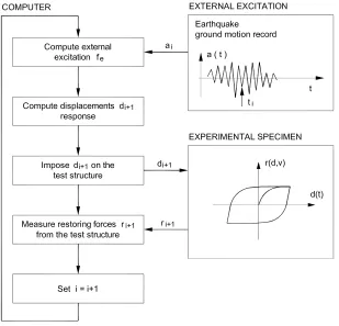
lo-cations. The detailed process of the PsD testing method is illustrated in Fig. 2.1.

(36)

generated earthquake ground acceleration history is used to compute the external

ex-citation ferunning the PsD algorithm. The displacement vector of the structure (where

the mass of the structure can be considered to be concentrated) is calculated using a

suitable integration method. The displacements are then applied to the test structure

by servo-controlled hydraulic actuators fixed to the reaction wall. Load cells on the

actuators measure the forces necessary to achieve the required displacements and

these restoring forces are returned to the computer for use in the next time step

calcu-lation (Pegon and Pinto, 2000; Bursi, 2008). Even though Eq. (2.1) can be expressed

Fig. 2.1: Flow of the PsD testing method

for any number of degrees of freedom (DoFs), it is not feasible to test large structures.

This is because the number of DoFs tested is determined by the number of available

actuators and some other laboratory facilities. Even for a simple structure, the mass

has to be concentrated in certain location through standard condensation techniques.

(37)

enough for their in-plane deformability to be ignored and most of the mass is

concen-trated in the floor slabs. However, earthquake loading often leads to severe damage

and unpredictable uncertainty only in parts of the structure. It would be much more

desirable to test the critical parts of the emulated structure while also the restoring

forces for the remainder are modelled in the computer. This is the main idea of the

PsD testing method with dynamic substructuring.

2.2.4 PsD testing method with dynamic substructuring

It was observed that during structural testing, damage (and therefore nonlinear

be-haviour) often occurred in specific, limited regions of an entire structure. Hence, the

substructuring technique was introduced to the PsD testing method by Dermitzakis

and Mahin (1985). With the aid of the substructuring methodology, a physical model

is built only of the part or parts where nonlinearity is expected (the PS) while the

re-mainder is computationally modelled (the NS). The principle of the method is similar

as the PsD testing method. The only difference is that the restoring force of the NS is

numerically modelled.

With the substructuring technique, the number of DoFs of the tested structure is

likely to be quite large. As far as utilized integrator is concerned, it was initially

ex-pected to use an explicit integration (Shing and Mahin, 1984). Solving large ODEs

system with an explicit integrator may lead to stability problem, which blocks the

application of the PsD testing to large-scale structural models. To overcome this,

Dermitzakis and Mahin (1985) proposed a mixed implicit-explicit algorithm based on

the work by Hughes and Liu (1978). Due to the increasing complexity of the tested structures, many efficient, unconditionally stable numerical algorithms were

devel-oped, such as Operator-splitting (OS) method (Nakashima, 1990), implicit Newmark

method (Dorka and Heiland, 1991) and the alpha method (Shing et al., 1991).

How-ever, the direct application of implicit integration algorithms to PsD tests has been

partially limited by the requirement to iterate with experimental substructures and

dif-ficulties in estimating the experimental tangent stiffness matrix. To implement implicit

integration methods, (Shing et al., 1991), (Bursi and Shing, 1996) adopted a modified

(38)

more detailed coverage of the development of numerical integration methods for PsD

testing with substructuring.

Before moving to the RTDS testing in the next subsection, another efficient

tech-nique, the so-called continuous PsD testing method is introduced here, in which the

loading rate is increased and the hold period is eliminated. This technique, by sus-taining a smooth motion and a continuous loading of the test structure, eliminates

or at least reduces force relaxation of structural materials. Moreover, capabilities for

fast rate or near real-time also partially allows for rate-dependent effects of the tested

structure. The new techniques for fast rate are built upon the same integration

meth-ods and principles developed for PsD testing in Subsection 2.2.3. As faster rate of

testing with no hold period are achieved, additional challenges arise in solving this

equations of motion: i) the use of shorter time step; ii) the adoption of parallel

solu-tion procedure; iii) the higher requirement to dealing with the inherent control error

and response lag of servo-hydraulic systems. For this technique, Researchers at the

JRC, ISpra have made a considerable effort and substantial contributions on the de-velopment both on parallel integration algorithms (Buchet and Pegon, 1994; Pegon

and Magonette, 2002, 2005) and on control issues (Magonette et al., 1998).

2.2.5 Real-time testing with dynamic substructuring

When rate-dependent effects are of importance, the continuous PsD testing needs to

be extended to RTDS. This approach is similar to PsD testing with substructuring, but

with the testing proceeding in real time. The test principles can be better understood

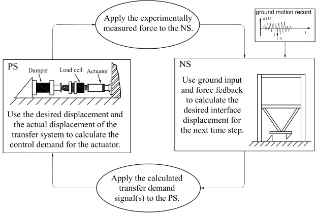
through a simple two-story building with a damper device as shown in Fig. 2.2. As shown in the figure, the tested structure is divided into a test specimen (the damper,

which is expected to reduce the response of the overall structure and make

possi-bly less damage to the main structure during the test) and a surrounding numerical

substructure. By imposing compatibility and equilibrium conditions at the interface,

the substructures are mode to interact possibly in real time, in order to emulate the

dynamic behaviour of the overall structure. In detail, the test process starts from time

integration in the numerical substructure, with the measured force from the PS and

(39)

and then sent to the actuator to advance the PS. At the end of the time-step the

ac-tuator loads and positions are measured and fed back to the numerical model. This

loop is completed at each time incremental until the test is completed. This technique,

Fig. 2.2: Control loop of the RTDS testing method

since it was developed by Nakashima et al. (1992), has been undergoing a rapid

de-velopment world-widely both on control issues and integration methods (Nakashima, 2001; Williams and Blakeborough, 2001; Blakeborough et al., 2001). The increasing

interest in RTDS testing is motivated by two major features: i) real time simulation

enable the technique to consider rate-dependent phenomena such as strain rate

ef-fects on material properties or viscous damping forces for specific dissipative devices;

ii) substructuring technique makes the possibility of large-scale structural tests with

common laboratory facilities.

Meanwhile, real time testing requires rapidly imposing high loads or accurate

dis-placements over a range of frequencies. This, on the one hand, imposes high

require-ment for efficient integration methods which will be detailed in the next section. On

the other hand, it is a difficult task to make the actuator(s) execute exactly and

con-tinuously within a shorter period. In the case of the work presented in the thesis, the

(40)

rapidly from the NS to the PS. Also, the restoring forces measured form the PS must

be quickly fed back to the NS. Communications between these two substructures

are thus of paramount importance which, to some extent, determine the accuracy

or the reliability of RTDS tests. To obtain desirable communications, efficient control

schemes are required to minimize propagations of the experimental error during tests

and to compensate for the actuator dynamics which is beyond emulated structures.

Historically, Horiuchi et al. (1996) pointed out that the effect of the effect actuator

dy-namics may introduces negative damping for a linear system which may cause the test to become unstable, and utilized polynomial extrapolations to compensate for

it. From then the effect has been gained sufficient attention by many researchers

working on this subject (Horiuchi et al., 1999; Nakashima and Masaoka, 1999). Also,

some control approaches were developed to considering actuator dynamics (Darby

et al., 2001; Wagg and Stoten, 2001; Neild et al., 2005; Bursi, 2007). A fuller review

of the delay compensation schemes used for RTDS testing is given in Chapter 5 of

the thesis (Bonnet, 2006).

2.3 Integration methods for RTDS testing

In a RTDS test, finite element method is used to discretize the problem spatially.

The resulting dynamic equations of motion are a system of second-order Ordinary Differential Equations (ODEs):

M ¨u+f(u ¨u) =fe (2.2)

wherefis the assembled resisting force vector (which depend on the structural

dis-placement vector and velocity vector). If the applied loads are entirely due to ground

acceleration, the external force vector fe on the right-hand side of (2.2) can be

re-placed by the following expression.

fe=−MB ¨ug (2.3)

where B is the ground acceleration transfer matrix and ¨ug is the specified support

(41)

When considering the substructuring methodology, the resisting force vector can

be divided by means of differential partitioning (Bursi, 2008) as follows

f(u ü) =fn(u ü) +fp(u ü) (2.4)

where subscript n refers to the NS and subscript p stands for the PS. Note that the

time integration methods discussed in this section are mainly used for the so-called

monolithic integration method. If the experimental mass is negligible, the resisting

force vector of the PSfp _{is directly measured from the specimen by a data}

acquisi-tion system. Otherwise, the force vector measured includes the inertial forces of the

specimen. In order to avoid duplication, one way is to compensate for the initial forces

by measuring the corresponding acceleration. Another way is to remove components with respect to the mass of the NS from the matrixM. The RTDS test related to the

coupled spring-pendulum system in Chapter 4 adopts the latter way.

Since the RTDS testing was developed, various integration methods have been

implemented and validated in the past decade. In order to review them systematically,

they are classified into three groups: explicit methods, implicit methods and linearly

implicit methods. For an explicit method, the target displacement solution at ti+1can be entirely expressed by known solutions such as the current state at ti and k −1

previous solution states earlier, i.e.,

ui+1 =f(ui,˙ui,¨ui, ... ,ui−k+1,˙ui−k+1,¨ui−k+1) (2.5)

where k indicates that the method belongs to k-step method. Note that in order

to distinguish them from linearly implicit methods, the right hand side of 2.5 does

not involves tangent stiffness matrix or its approximation. The advantages of explicit methods are that they are computationally efficient, easy to implement, and fast in

their execution. However, they are conditionally stable -the second Dalquist barrier

(Lambert, 1991, p.243)-. This indicates that the time step used frequently has to

satisfy stability condition other than accuracy requirement, especially in presence of

high-frequency components. In other words, explicit integration method is not suitable

for stiff problems which have natural frequencies with different scales.

For an implicit method, the target displacement solution at ti+1not only depends on known solutions as explicit methods but also unknown solutions at ti+1, i.e.,

(42)

Most of implicit methods are unconditionally stable, thus rendering suitability for stiff

problems. It also implies that the choice of time step is due to the accuracy

require-ment, because this type of methods is stable for any time step. However, they are

computationally more complex than explicit methods, often requiring an iterative

so-lution process. Moreover, iterations may introduce spurious loading cycles for the PS

and/or unloading process within a step which therefore causes non-realistic stiffness

measurements.

Besides explicit methods and implicit methods, another type of integration methods

is of interest in RTDS tests, linearly implicit methods. The methods are called linearly

implicit in that they require only a single linearization and matrix decomposition per time step. This type of methods have explicit expression of target displacements as

(2.5). But they also have some properties of implicit method, A-stability or L-stability,

for the reason that single built-in iteration is included. A drawback of linearly implicit

methods is that evaluation of tangent stiffness matrix and its inversion is required

per time step. To solve this problem, users for RTDS testing frequently adopt initial

stiffness matrix (Chang, 2002) or other approximations (Bursi et al., 2008; Lamarche

et al., 2009).

In the following subsections a detailed review of time integration methods used for

RTDS is presented following the aforementioned classification. For each method, the

formulation is provided, and its stability, accuracy and efficiency for RTDS testing are

detailed.

2.3.1 Central difference method

The central difference method (CDM) is the most popular time integration method for

RTDS testing, especially RTDS testing applied to a Single- or Multiple-DoF systems

(Nakashima et al., 1992; Horiuchi et al., 1999; Nakashima and Masaoka, 1999; Darby

(43)

2005). It is mathematically described by:

M ¨ui+C ˙ui+ri =fe,i

¨ui =

1

∆t2(ui+1−2ui+ui−1)

˙ui =

1

2∆t (ui+1−ui−1)

(2.7)

where∆tis the time step chosen.

The CDM is explicit but conditionally stable. The stability limit of the CDM is

ωmax∆t ≤2whereωmaxis the greatest natural frequency of the tested structure.

Math-ematically, the method is second-order accurate, with no dissipation but slight period

delay with sufficiently small time step. For RTDS testing, (Nakashima and Masaoka,

1999) proposed that the choice of used time step satisfiesωmax∆t ≤ 0.3 ∼ 0.4 for

achieving accurate responses.

To implement the CDM for RTDS testing, inserting the acceleration and velocity

expressions into equilibrium equation yields a formula of target displacement in terms

of known solution of the two previous steps (Darby et al., 2001). The expression

of the target displacement contains an inverse term but no time-dependent tangent