Spatiotemporal modelling and mapping of the bubonic plague epidemic in India

Open Access

Methodology

Spatiotemporal modelling and mapping of the bubonic plague

epidemic in India

Hwa-Lung Yu and George Christakos*

Address: Department of Geography, 314 Storm Hall, San Diego State University, 5500 Campanile Drive, San Diego, CA 92182-4493, USA

Email: Hwa-Lung Yu - [email protected]; George Christakos* - [email protected] * Corresponding author

Abstract

Background: This work studies the spatiotemporal evolution of bubonic plague in India during 1896–1906 using stochastic concepts and geographical information science techniques. In the past, most investigations focused on selected cities to conduct different kinds of studies, such as the ecology of rats. No detailed maps existed incorporating the space-time dependence structure and uncertainty sources of the epidemic system and providing a composite space-time picture of the disease propagation characteristics.

Results: Informative spatiotemporal maps were generated that represented mortality rates and geographical spread of the disease, and epidemic indicator plots were derived that offered meaningful characterizations of the spatiotemporal disease distribution. The bubonic plague in India exhibited strong seasonal and geographical features. During its entire duration, the plague continued to invade new geographical areas, while it followed a re-emergence pattern at many localities; its rate changed significantly during each year and the mortality distribution exhibited space-time heterogeneous patterns; prevalence usually occurred in the autumn and spring, whereas the plague stopped moving towards new locations during the summers.

Conclusion: Modern stochastic modelling and geographical information science provide powerful means to study the spatiotemporal distribution of the bubonic plague epidemic under conditions of uncertainty and multi-sourced databases; to account for various forms of interdisciplinary knowledge; and to generate informative space-time maps of mortality rates and propagation patterns. To the best of our knowledge, this kind of plague maps and plots become available for the first time, thus providing novel perspectives concerning the distribution and space-time propagation of the deadly epidemic. Furthermore, systematic maps and indicator plots make possible the comparison of the spatial-temporal propagation patterns of different diseases.

Background

Epidemics can have profound effects upon human popu-lations, states and governments [1]. The bubonic plague started in southern China in 1855, but the situation was rather ignored by the rest of the world (in part because of the 1851–1864 Taiping rebellion in the area; [2]). But,

when the plague reached Hong Kong and Canton in 1894, western authorities decided to intervene to avoid a world-wide epidemic [3]. Unfortunately, they were only partly successful, as the epidemic spread primarily in India with serious consequences [4,5]. It took more than 10 years to conclude that the bubonic plague was a disease

transmit-Published: 17 March 2006

International Journal of Health Geographics2006, 5:12 doi:10.1186/1476-072X-5-12

Received: 09 January 2006 Accepted: 17 March 2006

This article is available from: http://www.ij-healthgeographics.com/content/5/1/12

© 2006Yu and Christakos; licensee BioMed Central Ltd.

ted by fleas. About 10% of the infected fleas develop esophagus and gizzard blockage due to the highly abnor-mal reproduction of bacteria after sucking blood from infected rats. The blockage makes the fleas hungry, since the blood cannot reach the intestines for digestion, which implies that the fleas start biting at a higher rate. The bubonic plague mechanism requires at least one species of rodents that is resistant to the bacteria and another one that is not. The resistant rodents keep the disease endemic by hosting the infested fleas. The infection is passed from the fleas to their victims by means of the blocked fleas that regurgitate infected blood at biting. As the sensitive rodents are infected, they die. Then the fleas, facing a shortage of their preferred host, move onto people, thus triggering the epidemic. The disease makes its appearance in humans within a week following the biting by infected fleas. The causative agent of the bubonic plague is the Yersinia pestis (Y. pestis) bacillus. Multiplication of the bacteria produces the characteristic "bubo" (swollen, painful lymph node). Bacteremia follows, causing death in about 75% of those affected.

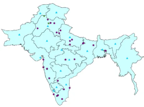
The Indian bubonic plague characteristics (seasonal effects, the role of rats and fleas etc.) have been well doc-umented [6]. However, most investigations focused on selected cities to conduct different kinds of studies, such as the ecology of rats. As a result, the monthly or yearly mortality information contained in the bubonic plague database refers only to these cities; also, most of the plague data were organized at the provincial scale (the data distribution is shown in Figure 1). To our knowledge, no detailed maps exist providing a composite space-time picture of the disease propagation characteristics across

space-time. In order to produce systematic space-time maps of the epidemic, it is necessary to use a rigorous methodology that makes optimal use of the provincial monthly mortality information to support a monthly database construction. At the same time, the various uncertainty sources characterizing the propagation of the epidemic must be adequately accounted by the space-time methodology.

Results

Spatiotemporal maps of bubonic plague mortality

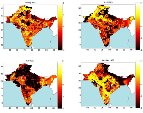
Monthly mortality rates for the period September 1896-October 1906 were collected or generated using the pro-posed space-time method, leading to a complete set of 122 mortality maps in space-time. The maps allow dis-playing and studying in detail the geographical distribu-tion, temporal evolution and seasonal effects of the deadly epidemic. Due to space limitations, a small subset of these maps is plotted in Figure 2 (although a complete set is available). The space-time method generates the complete mortality pdf, f_K, at each space-time point over India; from these pdf, characteristic values (mode, mean, median) can be derived. The maps in Figure 2 represent the mean values, , of the corresponding pdf.

The territory shown in these maps is India in the 1900s, excluding a part of Burma. For historic reasons, the pro-vincial information in the database is slightly different from the information shown in the maps. E.g., the Bengal presidency was divided into 3 provinces: Bihar/Orissa, Bengal, and Assam [7]. The reason for this database divi-sion is that in 1900 these provinces were still parts of the Bengal presidency. However, in 1905 the Bengal presi-dency was partitioned into Bengal and Assam, whereas in 1912 Bihar and Orissa formed a new province. The monthly provincial mortality provided in [8] was in accordance with the later partition of provinces. The gen-erated bubonic plague maps describe the varying mortal-ity spread throughout India and during different time periods. On the basis of these maps, several observations are made below concerning the space-time distribution and propagation of the bubonic plague epidemic throughout India.

The bubonic plague started at a port: Bombay City (1896). Then, it gradually moved inland, like a cloud of varying size, depending on the geographical area (the cloud anal-ogy aims to describe an epidemic propagation advancing but at the same time disappearing and reappearing in infected areas). Although most of India was visited by the plague (also, Figure 3 below), during the first decade of the epidemic a few regions were spared: (i) Assam (it is believed that life style and the local population

condi-ˆ _,

m_kmean

The bubonic plague data distribution Figure 1

tions provided an unfavorable environment for the Rattus rattus to spread the plague) [7: 348–351]. (ii) Eastern and southern parts of the Madras presidency (the specific spe-cies of fleas limited the bubonic plague infection only among the rats) [7: 357–360]. (iii) Baluchistan in the western part of India, which today is Pakistan (because of its mountainous terrain, the temperature in Baluchistan usually falls to 0°F during the winter which prevents the fleas from breeding).

As the mortality patterns show, in its first year (1896) the plague stayed close to the Bombay City, moving only slightly along the coastal line. After the initial outbreak, the bubonic plague moved East and South into the Bom-bay Presidency (September 1897); the epidemic hit was severe in parts of this area and lasted until February 1898. At the same time, the northern part of the Bombay Presi-dency exhibited relatively lower mortality. The second

epidemic wave receded in early summer 1898. In June 1898 the mortality values rose dramatically in the south-ern part of the Bombay Presidency and the epidemic lasted until the following spring. By September 1898 the bubonic plague had spread throughout the entire Bombay Presidency; in fact, for the first time it went past the Presi-dency boundaries and attacked neighboring areas, namely Hyberabad and Mysore.

In early spring 1899 the Bombay city suffered another bout of the epidemic that lasted until May. Although the epidemic showed signs of temporary recession, it started rising again in June 1899 at the southern parts of the Bom-bay Presidency. During the rest of the year the epidemic spread throughout the entire Bombay Presidency. The peak of the epidemic was observed in September 1899 and by December the infected area was negligible in most of the region. Nonetheless, in the western coastline and Space-time mortality rate maps during 1902–1903

Figure 2

close to the Bombay city, the plague rose again and remained consistently strong starting in January 1900 and ending in May 1900, thus showing a repeating pattern of two peaks per year (unlike most other regions that experi-enced only one peak per year). The space-time maps indi-cate that the first visit of the epidemic in the Bengal province (Bihar/Orissa) occurred during March 1900. On

the basis of the mortality numbers, one may deduce that the infection was relatively mild compared to that of the Bombay city area (Bombay city, Poona, Kirkee etc.). In the Bombay city the epidemic ended the month of May 1990. In July, however, the epidemic re-emerged in the southern part of the Bombay Presidency (Belgaum). Also, the epi-demic spread to the North of the Bombay city in August, Space-time area epidemic maps (1896–1906)

Figure 3

and the following September it moved East toward Hyderabad and Mysore. The epidemic slowed down in the Bombay Presidency during the month of December 1900.

In the beginning of 1901, the epidemic first passed the Mysore area and reached the Madras Presidency (Vaniya-mbadi). As the mortality maps show, the bubonic plague also recurred in the Bengal area and was more severe this time. The epidemic in the Bombay city had never com-pletely disappeared by the end of 1900, and it made a strong reappearance in February 1901. Following the rel-atively calm months of May and June, high mortality was recorded in southern Bombay (August 1901), followed by the severe infection of the entire Bombay Presidency. By the end of 1901, the severity of the disease was reduced in the southern part of the Bombay Presidency, but the Bom-bay region displayed high mortality during December 1901. In the meantime, the epidemic re-emerged in the Madras Presidency (October 1901). During 1901 winter several other provinces in northern India had been visited by the plague (Punjab, United Provinces, Bihar/Orissa).

The space-time maps show that in early 1902 the bubonic plague became, once more, a severe epidemic in various parts of India. In Bombay city the epidemic reached its mortality peak during February 1902 and ended in June 1902. In northern India (Punjab and United Provinces) the mortality peak occurred during March-April and it also ended in June 1902. As for the southern India (inland Madras Presidency), the disease peak was observed in December 1901 and January 1902, whereas the plague receded in May 1902. Similar to the epidemic pattern of 1901-1902, the southern part of the Bombay Presidency was also the first place in which the plague recurred in August 1902, whereas peak mortality was again reached in Bombay city and the inland Madras Presidency during December 1902. The plague then moved to the North occupying the entire Bombay, Punjab, and United Prov-inces. In December 1902 the first infection took place in the Central Provinces. Interestingly, the mortality distri-bution in Bombay city demonstrated a similar behavior, which consisted of an increasing trend during the winter that reached a peak in the following spring and then ended in late spring of the same year.

The mortality maps reveal that in southern India the plague lasted until May 1903 and in northern India until June 1903. Following the last epidemic in Punjab, a related pattern was repeated in 1903. The mortality peak of bubonic plague occurred in the southern Bombay Pres-idency during September of the same year. In November 1903 the epidemic spread toward the inland Madras Pres-idency and the northern part of Bombay PresPres-idency (Surat). Following this trend, the plague subsequently moved into the Central Provinces and the Bombay city

(December 1903-January 1904), and then went further up north to the United Provinces and Bengal area (March 1904) and Punjab (April 1904).

In early spring 1904, the bubonic plague had infected almost the entire northern India (Punjab, Rajputana, United Provinces, Bengal and Kashimir). Punjab was the most severely hit province and the one where the epi-demic lasted the longest. In contrast, Rajputana suffered a relatively milder blow from the plague. From a topo-graphical viewpoint, the Thar desert, the Mount Abu, the Aravalli range, and the tropical forests in this region are not propitious to fleas or rats commuting. However, Pun-jab is an extensively flat plain, open to the east and south, and its climate and temperature are favorable for flea breeding. In south India (Bombay Presidency, Mysore and Hyderabad) the plague re-appeared in July 1904 and then started moving north. Following the pattern of the previ-ous years, the epidemic peaked at the southern Bombay Presidency during September; then, in late 1904 it went north into Bombay city, the Surat region, Central India and the Central Provinces; during March-April 1904 the epidemic moved to Punjab, United Provinces and Bengal reaching its mortality peak. A difference with the previous years was that, this time, the epidemic did not infect the Madras Presidency.

On the basis of the mortality maps of the years 1904– 1905, one observes that the epidemic spread across India from south to north. High mortality rates were recorded at the Bombay Presidency, Punjab, United Provinces and Bengal. Despite this trend, infection rates were relatively modest in Mysore, Hyderabad, Central India, Rajputana and the Central Provinces (except in the Nagpur city). The topography of India may explain the close correlation between devastation degree and the terrain variability. The hills and mountains of central India are a rather unfa-vorable migration environment for fleas and rats com-pared to the flat plains of the Bombay Presidency, Punjab, the United Provinces and the Bengal Presidency. In the fall of 1905, the Bombay Presidency had a comparatively mild epidemic. After that, the disease moved into north-ern India.

by the developed transportation means may have been an influential factor in the space-time spread of bubonic plague. The railway map of India in 1893 offers some hints concerning the close association between the rail-way system and the epidemic distribution. In the early 1900s, India was divided into British India (Bombay Pres-idency, Punjab, United Provinces, Bengal Presidency etc.), as well as other native India states (Hyderabad, Mysore, Central India etc.). GIP offered good connections for most of the British India region; however, the native India parts were more difficult to reach than the British India region. Therefore, the transportation infrastructure may provide some insight on why British India generally suffered more by bubonic plague than the native India. The railway also increased the spreading speed of the bubonic plague dur-ing 1902–1903, as is noticed in the space-time mortality maps of these years. Cawnpore (a railway junction in the United Provinces) and Bhagalpur (the administrative and marketing center in Bihar with railroad connection) were both infected by more severe bubonic plague attacks than the remaining areas in the region.

Spatiotemporal maps of geographical evolution

The selection of maps in Figure 3 shows the geographical evolution of the epidemic during different times (a com-plete set of more than 120 maps is available but is not plotted here, due to space limitations). The maps are derived on the basis of the mortality distributions availa-ble during the construction of the spatiotemporal mortal-ity maps. Let P[M_p > 0.01%] denote the probability that mortality M at a given space-time point p exceeds the 0.01% threshold. A location is considered infected when P[M_p > 0.009%]>0.65 at that location. Several alternative sets of maps can be constructed by choosing different mortality and probability thresholds. This flexibility of geographical information science ([10]) allows one to focus on important space-time features of the bubonic plague epidemic.

According to the geographical evolution maps the disper-sion of the bubonic plague in India would either slow down or come to a complete halt from April to August in each epidemic year. Another feature of the disease evolu-tion made apparent from the mortality maps is that the epidemic tended to stop or slow down during certain peri-ods of the year, even if at the time the epidemic would tend to restart or would still be going through a severe stage in a region.

Spatiotemporal epidemic pattern

The temporal variation of the total infected area indicator, T(t), for the Indian epidemic is shown in Figure 4. During its entire duration, the bubonic plague invaded new geo-graphical areas at an average rate of about 4 × 104 _km2_/

month. Considered in the context of local time intervals,

the T-curve of the bubonic plague spread consists of two parts (Figure 4): The slope of the one part is close to zero, which signifies a halt in the plague spread; the second part, however, exhibits a steep slope indicating that the bubonic plague would spread very fast at a time of high activity. In fact, the propagation rate during the months of December 1901-May 1902 is the fastest observed for the epidemic during any time period.

An interesting phenomenon is observed in Figure 5 that

plots the indicator T(t) vs. time. This quantity can be

thought of as the "instant speed" of the total infection area expansion. The rate for the bubonic plague changed sig-nificantly within each year. The variation of the "instant rate" for the plague epidemic indicates that it exhibited a seasonal effect. The five most aggressive spread rates of bubonic plague occurred in March 1897, November 1898, March 1900, January 1902, and February 1903; whereas the four less aggressive rates occurred in Novem-ber 1897, February 1898, March 1901, and February 1904. Before each large outburst, it took 1–2 years for bubonic plague to preserve its energy, and for that time it would stay static at the same locations. The huge expan-sion bursts of the total infected area T(t) took place mainly during the spring. Similar observations can be

made about Figure 6, which plots T(t)1/2 _{vs. time}

pro-viding a measure of the speed of the total infected area T(t).

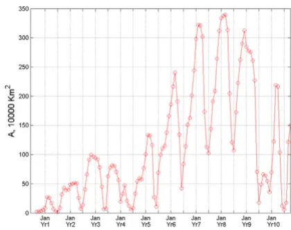
According to the geographic evolution maps of the epi-demic, it is evident that the bubonic plague ravaged across almost its entire space – the subcontinent of India. From the plot of A(t) vs. t (Figure 7) it is clear that bubonic plague grew larger and larger during the years, and at cer-tain times it occupied most regions of India. The reason for this is that the plague followed a re-emergence pattern from its prior infection in the geographical locations. The plot of N(t) vs. t in Figure 8 gives some insight about the relocation mechanism for the bubonic plague epidemic. The ragged bubonic plague curve shows that the plague would change its location twice a year, i.e., almost every spring and fall. The area-averaged monthly mortality var-iation plot for bubonic plague is shown in Figure 9. The plot is in agreement with the results of [11], which had concluded that the plague mortality during the years 1900–1905 did not exceed 0.4% per year.

Moreover, the epidemic indicators allow some interesting comparisons of the Indian epidemic vs. the medieval Black Death epidemic in Europe (for a detailed discussion of the spatiotemporal characteristics of Black Death, see [10]). E.g., during the bubonic plague's first 40 months

d dt

there were only 3 times when the mortality rate was raised to levels comparable to those of the medieval Black Death; during the rest of the time, the plague either remained static geographically or it completely disap-peared. As was discussed in previous sections, bubonic plague was stale in the summer and active in the spring and fall, whereas the geographical Black Death evolution tended to be slower during winter. Bubonic plague fatali-ties in India were minimal to none during the dry and hot months of April-August [7]. On the contrary, the Black Death casualties merely slowed down during the cold winter months; moreover, after the first summer, Black Death reached a global maximum that was followed by maxima of decreasing levels, whereas bubonic plague kept reaching new heights for several years.

Discussion – conclusion

We introduced rigorous stochastic modelling in the spati-otemporal analysis of the bubonic plague epidemic in India during the years 1896–1906. We discussed geo-graphical information science concepts and techniques underlying the study of the bubonic plague patterns of growth.

A variety of informative space-time maps of mortality rates and geographical disease evolution were generated that accounted for multi-sourced databases and uncer-tainty conditions. A series of epidemic indicators were plotted that offered meaningful characterizations of the spatiotemporal disease distribution.

The bubonic plague in India exhibited strong seasonal and geographical features. During its entire duration, the plague continued to invade new geographical areas, while it followed a re-emergence pattern at many localities; its

rate changed significantly during each year and the mor-tality distribution exhibited space-time heterogeneous patterns; prevalence usually occurred in the autumn and spring, whereas the plague stopped moving towards new locations during the summers.

Among other things, the epidemic maps and indicators make possible the comparison of the spatiotemporal characteristics of different diseases. Such comparisons could detect discrepancies in the spatiotemporal patterns of the epidemics; it is then left to specialized investiga-tions to seek substantive and biologically plausible expla-nations of these discrepancies.

Methods

Stochastic spatiotemporal modelling

Methodologically, the bubonic plague distribution across space-time is conceptualized as a stochastic epidemic sys-tem and the bubonic mortality rates are represented as spatiotemporal random fields (S/TRF). The geographical information technology is subsequently implemented to map these rates in the composite space-time domain of the epidemic. This is a synthetic methodology ([10]) that provides the means to understand the nature of space-time disease processes among populations of individuals.

Our understanding of past epidemics is uncertain because the information available is inconclusive and to some degree inaccurate (on occasion the available evidence appears contradictory). Therefore, in modern epidemic studies the S/TRF theory is the main tool of stochastic modelling. The S/TRF theory adequately contextualizes and evaluates the uncertainty sources concerning the space-time distribution of an epidemic. The values of a Temporal variation of the dT/dt-indicator for bubonic plague Figure 5

Temporal variation of the dT/dt-indicator for bubonic plague. Temporal variation of the T-indicator for bubonic plague

Figure 4

disease distribution are attributed to spatiotemporal points under conditions of uncertainty, and multiple real-izations are considered that account for composite space-time disease variations together with the associated prob-ability models. A mathematical presentation of the S/TRF theory can be found in [12,13]. Before proceeding with our discussion of the theory, let us note that mortality dis-tribution was selected as the space-time variable character-izing the bubonic plague epidemic in India, since the available information is related (directly or indirectly) to mortality. In particular, based on data availability, the monthly mortality rate is defined as M_monthly = D_monthly/TP

= RD_monthly , where D_monthly, D_yearly are the numbers

of plague deaths per month and per year, respectively, TP is the total population and R is the ratio of yearly plague deaths over the total population, and can be represented as R = Dyearly/TP.

Let p = (s, t) be a point in the space-time domain; s

denotes the spatial location and t the time instant under consideration (months, years etc.). In the S/TRF context one views space and time in a composite way: as a single block of space-time. In this sense one may distinguish between the separable space-time domain considered in most statistical analyses vs. the composite space-time domain of S/TRF analysis. Basically, an S/TRF Mp = Ms,t representing mortality distribution is a collection of reali-zations (possibilities, potentialities) for the disease values in space-time. The multiplicity of realizations allows S/ TRF to account for uncertainty sources and adequately represent the spatiotemporal variation of bubonic mortal-ity in India. Stochastically, the S/TRF model is fully

char-acterized by its probability density function (pdf), f_KB, generally defined as

where the subscript KB denotes the knowledge base uti-lized to construct the pdf (the pdf depends explicitly on the points p₁, p₂, ..., but we do not explicitly show this for convenience). Stochastic modelling of disease distribu-tions with complicated space-time patterns entails deter-mining the S/TRF from a single realization. Trend-free (spatially homogeneous and temporally stationary) S/TRF have been assumed widely in health geographics, because they are efficient for explicit and numerical calculations. However, the homogeneous-stationary model is not the best option for phenomena with large and complicated space-time variabilities.

In light of these issues, a class of heterogeneous S/TRF has been proposed by [12] that is considerably more general than the restricted class of homogeneous-stationary S/ TRF. This new class is capable of handling complicated space-time variabilities of any size based on the following intuitive idea: The variability of an S/TRF can be character-ized by means of its degree of departure from homogene-ity and stationarhomogene-ity. This departure can be determined by a mathematical operation, in the following sense. Let Qν/ µbe a space-time operator that transforms the S/TRF Mp into a homogeneous-stationary field Y_p by annihilating heterogeneities of degrees νin space and µin time, i.e.,

Qν/µ[Mp] = Yp (2)

In this case, the mortality field M_P is said to be an S/TRF with spatial and temporal heterogeneity orders νand µ, respectively (S/TRF-ν /µ; [12,14]). The S/TRF-ν /µoffers a

D_yearly−1

PKB[m1≤Mp1≤m1+dm m1, 2≤Mp2≤m2+dm2, ... ]=fKB(m m1, 2,...)dm dm1 2.... ( )1 Temporal variation of the A-indicator for bubonic plague Figure 7

Temporal variation of the A-indicator for bubonic plague. Temporal variation of the dT1/2_{/dt-indicator for bubonic}

plague Figure 6

general theoretical model of the mortality distribution that expresses the way causal influence is propagated in space-time and gives information about the bubonic plague dynamics at the scale of interest. For epidemic sys-tems that evolve within domains containing complicated boundaries and trends, the departure of the random field from homogeneity-stationarity is expected to vary geo-graphically. It is, thus, meaningful to construct local Qν/µ

-operators that generate homogeneous-stationary random fields Y_p within local neighbourhoods Λ, instead of seek-ing global representations.

In practice, various choices of Qν/µ-operators are possible,

thus allowing considerable flexibility in the definition of the S/TRF-ν/µ. Indeed, the spatiotemporal trend of the mortality distribution M_p inside each local neighborhood

Λ of the epidemic system may involve various functions with space-time coordinates (polynomial, exponential, trigonometric etc. functions). For the purposes of the cur-rent bubonic plague study, an efficient Q_ν/µ-operator is one that annihilates local heterogeneities involving com-posite space-time polynomials, P_ν/µ, of degrees νin space and µin time. The parameters νand µprovide a quantita-tive assessment of the rate of change of the functions mod-elling mortality patterns. E.g., the smaller the P_ν/µ, degrees, the smaller the values of νand µThe ν, µalso offer infor-mation about the stochastic model underlying the epi-demic system. E.g., these parameters may determine how "far away" in space and "deep" in time the operator searches for information about the mortality field.

Mortality correlations across space-time are characterized by the ordinary spatiotemporal covariance c_M(p, p') between any pair of points p and p'. This covariance is nonhomogeneous in space and nonstationary in time,

and according to the S/TRF- ν/µ, theory it can be decom-posed as

c_M(p, p') = κ_M(p - p')+ Pν/µ, (3)

where κ_M is called the generalized spatiotemporal covari-ance, and p - p' = (s - s', t - t'). An important feature of this mortality field model is that only the κ_M is required in spa-tiotemporal mapping. The κ_M can be expressed in terms of the residual ordinary covariance cY, so that given the form of c_Y, the corresponding κ_M is derived. Hence, the class of generalized space-time covariances is richer than that of ordinary ones.

Knowledge bases

In epidemic studies one often needs to integrate multiple sources of information, depending on the situation. In this work, the following knowledge bases (KB) are consid-ered: the general KB, (core knowledge about the

dis-ease), the specificatory KB, (site-specific hard and soft, instrument- and/or survey-based data), and the integra-tion KB, (the union of the - and -KB).

In principle, the -KB accounts for existing scientific knowledge (theoretical models, epidemic laws etc.), but also other kinds of useful knowledge that are relevant to the epidemic system under consideration. In the present study, the scientific part of the -KB includes the S/TRF-ν/µ, theoretical model representing dependence of bubonic plague mortality across space and time (in terms of the heterogeneity orders and generalized covariance).

 

  





The areal-averaged monthly mortality rates of bubonic plague vs time

Figure 9

The areal-averaged monthly mortality rates of bubonic plague vs time.

Temporal variation of the N-indicator for bubonic plague Figure 8

Region-wide S/TRF parameters ν, and µ, offer insight into space-time epidemic variations across India. The calcula-tion of the parameters in practice is made in terms of a computational procedure discussed in detail in previous publications (e.g., [13,15]). Maps showing the regional-ized ν - µ, distribution over India (e.g., during the year 1903) are shown in Figure 10, thus providing information about the relative trends of mortality in space-time (ν- µ >0 implies higher degree spatial trends; ν- µ<0 implies

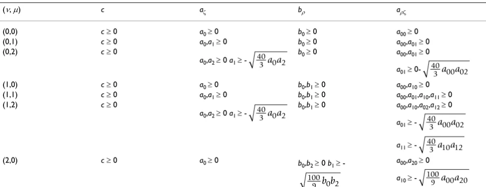
higher degree temporal trends). Not only the spatial order ν changes in space, but the temporal order µ varies in space, as well. Spatial and temporal trends are interre-lated, since the geographical propagation of the plague is also affected by temporal mechanisms. Theoretical κX models assumed to express the space-time dependence of bubonic plague mortality are shown in Eq. (4) of Table 1. The coefficients c, a_ζ, b_ρand a_ρζ, of the models (4) must satisfy the permissibility conditions of Table 2. The values

Table 1: Generaized covariance, κX, models.

κM( , )rτ =cδ δr τ+δr∑ςµ=0(−1)ς+1aςτ2ς+1+δτ∑νρ=0(−1)ρ+1b rρ 2ρ+1

++ − = − ′ = − ′

( )

+ =

= ∑ + +

∑ ( )

, .

,

1 4

0

0 ςµ ρ ς 2 1 2 1

ρ ν

ρς ρ τ ς

τ

a r

r s s t t

Space-time maps of the ν/µdifference in 1903 Figure 10

of these coefficients vary, depending on the local space-time neighborhood Λ of the epidemic system considered.

The -KB includes various information sources relevant to the Indian bubonic plague, starting the year 1896 [6,8,16]. The following terminology is used: Ps,t =

popu-lation; , = yearly and monthly city mortalities

rates; , = yearly and monthly provincial

mortal-ity rates; , = number of city deaths per year and

per month; , = number of provincial deaths per

year and per month. Also, the following parameters are

introduced: ;

, ; and

,

; with = average

numbers of city and provincial deaths per month. In light of the above considerations, the -KB can be effectively divided into several sub-groups, as discussed in detail in

the Appendix. The estimation of the values at each

geographical location and time instant involves certain uncertainty sources:

i. Uncertainty in the calculation of the ratios. This is

due to: (1) values at a given year must be calculated

from data, and (2) values are approximated

from the available provincial data at different times.

ii. Uncertainty due to the change of spatial support

(prov-ince vs. city). This situation occurs when: (1) the

val-ues are calculated from the data, or (2) the

values are calculated from the data.

iii. Uncertainty due to the approximate readings of the charts. This is the case when one seeks to interpolate between the chart values etc.

An elementary formula of monthly city mortality is

. Due to the incompleteness of the ,

and datasets, one should account for the

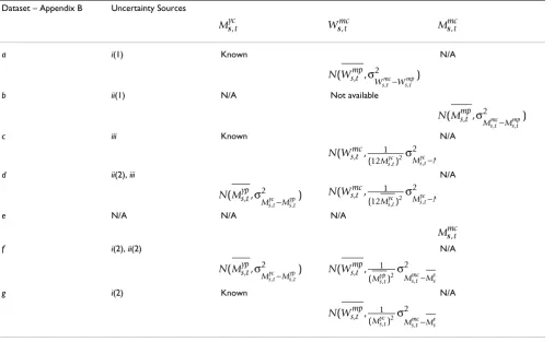
rele-vant uncertainties as described in Table 3 (the Gaussian law is used to define different uncertainty sources;

, and

= mean monthly ratio during the 1899–1906 at a

given province). Variances are due mainly to change of

support: the (respectively, )



M_syc_,t Mmc_s,t M_syp_,t Mmp_s,t

D_syc_,t Dmc_s,t D_syp_,t Dmp_s,t

Wsmc,_t =Dmcs,_t(Dsyc,_t) , −1 Wsmp,_t =Dsmp,_t(Dsyp,_t)−1

M_syc,_t =D_syc,_tPs−,1_t×103 M t D P yp

t yp

t

s, = s, s−,1×103

( )( )

, , , ,

Zsmc_t = Dmcs_t −Dmcs_t Dmcs_t −1

Zmp_s,t =(Dmp_s,t −D_smp_,t)(D_smp_,t)−1 Dmc_s,t,Dmp_s,t



Mmc_s,t

W_smc_,t W_smc_,t

W_smc_,t W_smc_,t

Mmc_s,t Mmp_s,t M_syc_,t

Myp_s,t

Mmc_{s t,} =M W_{s t}yc_{, s t}mc_, Mmc_s,t M_syc_,t W_smc_,t

ˆ _{[ ][ ]}

, , , , , , ,

Ws tmc = Zs tmcDmcs t +Dmcs t

∑

W_{s t}mp_,

σ_{W W}

s tmc, − s tmp,

2 _σ

M_{s t}mc_, −M_{s t}mp_,

2

Table 2: Permissibility conditions for the κ_X models of Eq. (4)

(ν, µ) c a_ζ bρ aρζ

(0,0) c ≥ 0 a0 ≥ 0 b0 ≥ 0 a00 ≥ 0

(0,1) c ≥ 0 a₀,a₁ ≥ 0 b₀ ≥ 0 a₀₀,a₀₁ ≥ 0

(0,2) c ≥ 0

a₀,a₂ ≥ 0 a₁ ≥

-b₀ ≥ 0 a₀₀,a₀₁ ≥ 0

a₀₁ ≥

0-(1,0) c ≥ 0 a₀ ≥ 0 b₀,b₁ ≥ 0 a₀₀,a₁₀ ≥ 0

(1,1) c ≥ 0 a0,a1 ≥ 0 b0,b1 ≥ 0 a00,a01,a10,a11 ≥ 0

(1,2) c ≥ 0

a0,a2 ≥ 0 a1 ≥

-b₀,b₁ ≥ 0 a₀₀,a₁₀,a₀₂,a₁₂ ≥ 0

a01 ≥

-a₁₁ ≥

-(2,0) c ≥ 0 a₀ ≥ 0 _b

0,b2 ≥ 0 b1 ≥ - a00,a20 ≥ 0

a₁₀ ≥

-40

3 a a0 2 40

3 a a00 02

40

3 a a0 2 40

3 a a00 02 40

3 a a10 12

100 9 b b0 2

expresses the uncertainty due to extrapolation from monthly provincial to monthly city ratios (respectively, mortality) at a given year (respectively, during 1899–

1906); is due to differences between the

avail-able yearly mortality city data and the mortality values

approximated by means of the charts; and is

the uncertainty due to differences between monthly mor-tality city values and the mean monthly mormor-tality provin-cial values.

For mathematical formalization purposes, the vector m_map

= (mhard, msoft, mk) denotes a possible mortality field reali-zation associated with the space-time point vector p_map =

(p_hard, p_soft, p_k) within each neighborhood Λ of the epi-demic domain. The mmap includes hard data (exact

obser-vations) m_hard = (m₁, ..., ) at points p_hard = (p₁, ..., ),

soft data (different kinds of uncertain observations) msoft =

( , ..., m_d) at p_soft = ( , ..., p_d), and the estimated mortality value χ_k at the point p_k. It is certainly possible to consider several mapping points in a neighborhood, in which case one is dealing with the vectors χ_k =

( ) and p_k = ( ).

The BME- ν/µtechnique

The geographical information technology involves a vari-ety of advanced space-time mapping techniques (for details, see [17]). In this study, the BME- ν/µ, technique (Bayesian Maximum Entropy of order ν/µ,) has been employed, which has a number of distinguished features including the following [15,18]:

- it accounts for the uncertainty features of the epidemic system in a composite space-time domain (unlike, e.g., spatial prediction techniques that focus on purely spatial domains);

- it imposes no restriction on the shape of the probability laws and the predictor forms (non-Gaussian laws and non-linear predictors are automatically incorporated);

- it assimilates a variety of core knowledge bases and site specific, multi-sourced datasets; and

- it derives several previous techniques of epidemic mod-elling (statistical regression, spatial prediction, kriging etc.) as its limited cases.

In light of these important features, the mapping of the mortality distribution can be more informative and realis-tic than the maps generated by conventional methods that do not possess the theoretical and applied qualities of BME-ν/µ, (most of the conventional methods can use lim-ited datasets, the linearity and normality restrictions apply etc.).

Within each neighborhood Λ of the geographical domain of the epidemic, the BME-ν/µ, mapping of the bubonic plague follows three knowledge synthesis stages:

a. At the so-called structural stage, a pdf is

con-structed on the basis of the -KB available, i.e.,

σ_{M M}

s tyc,− s tyc,

2

σ

M_{s t}mc_, −M_{s t}mp_,

2

md_h pd_h

md_h+1 pd_h+1

χ

χ



→ f_(mmap)=Bexp(−1₂mmapT κmap−1 mmap),

( )

(2,1) c ≥ 0 a₀,a₁ ≥ 0 _b

0,b2 ≥ 0 b1 ≥ - a00,a01,a20,a21 ≥ 0

a₁₀ ≥

-a₁₁ ≥

-(2,2) c ≥ 0

a₀,a₂ ≥ 0 a₁ ≥ - b0,b2 ≥ 0, b1 ≥

-a00,a02,a20,a22 ≥ 0

a₁₀ ≥

-a01 ≥

-a₁₁ ≥

-a21 ≥

-a₁₂ ≥ -Table 2: Permissibility conditions for the κX models of Eq. (4) (Continued)

100 9 b b0 2

100 9 a a00 20 100

9 a a01 21 40

3 a a0 2

100 9 b b0 2

100 9 a a00 20 40

3 a a00 02 4000

27 a a00 22 40

3 a a20 22 100

where , Q = Q(m_map) is the ν/µ,

-operator, z is the degree of freedom determined by the spatiotemporal trend, and κ_map is the generalized covari-ance matrix between the points pmap.

b. At the specificatory stage, the -KB considers hard and/or soft data (in the form of intervals and local proba-bility distributions). Operationally, transformations of

the following type are considered , where

and D denote, respectively, a specificatory operator

and information range determined by -KB. For illustra-tion, Table 4 presents some examples of -KB together

with the , D associated with the displayed soft data;

is the cumulative distribution function derived from

at the soft data points, I is a vector of mortality inter-vals at these points, and I_k is a vector of interval values at the estimation points themselves.

c. At the integration stage, the - and -KB are

com-bined to yield the integrated pdf at each mapping

point p_k using the operational Bayes formula

B= d z− QQT

−

(2 )

1 2

π



 _→{Ξ_, }D

Ξ   Ξ F_    f_

f m_k A d f

D data map

( )= −1

∫

( )

Table 4: Examples of soft data with integration domain D and operator .

D

Interval I m_soft

Probabilistic I _(m

soft)

Functional I ∪ I_k

(msoft,mk) Ξ

 Ξ

F_ F_

Table 3: Uncertainty sources and assessment of the various bubonic plague datasets.

Dataset – Appendix B Uncertainty Sources

a i(1) Known N/A

b ii(1) N/A Not available

c iii Known N/A

d ii(2), iii N/A

e N/A N/A N/A

f i(2), ii(2) N/A

g i(2) Known N/A

N/A = Not available

Myc_s,t Wsmc,_t Mmcs,t

N W_{s t}mp

W_{s t}mc W_{s t}mp

( _, , )

, ,

σ2 ₋

N M_{s t}mp

M_{s t}mc M_{s t}mp

( _, , )

, ,

σ2 ₋

N W_{s t}mc

M_{s t}yc M M

s t yc ( _, , ( _,) , 1 12 2

2σ ₋

N M_{s t}yp

M_{s t}yc M_{s t}yp

( _, , )

, ,

σ2 _{− N Ws t}mc

M_{s t}yc Ms tyc M

( _, ,

( _,) ,

1 12

2

2σ −

Mmc_s,t

N M_{s t}yp

M_{s t}yc M_{s t}yp

( _, , )

, ,

σ2 _{− N W}

s tmp

M_{s t}yp M M

s t mc s m ( _, , ( _,) , 1 2

2σ ₋

N W_{s t}mp

Ms tyc Ms tmc Msm

( _, ,

( _,) _,

1 2

2σ

where A is a normalization constant. From the integration pdf (6), various kinds of bubonic mortality estimates can be readily derived across space-time. E.g., the mean

esti-mate, ; and the mode estimate, . The

uncertainty of the mortality estimates may be assessed in terms of the mean squared estimation error, σk, at each space-time mapping point.

Competing interests

The author(s) declare that they have no competing inter-ests.

Authors' contributions

Both of authors were involved in the data analysis and processing, manuscript writing and editing.

Appendix 1

The Database of Bubonic Plague in India. The -KB of the bubonic plague epidemic in India is effectively divided into seven sub-groups:

(a) Dataset consisting of and ratio values

derived on the basis of the information available in [8].

The data were decomposed into values by

means of = . For cities in the Punjab

region, the values were calculated directly from the

number of plague deaths and the provincial

popula-tion P_s,t available in [6] (1912: 105).

(b) Dataset including values ([8]). Monthly

mortal-ity is defined as = . The data are

available starting July 1898; thus, ratios are

availa-ble after 1899.

(c) Dataset consisting of values ([6], 1912: 258) and

the chart of the ratios ([6], 1908: 301). Plague

mortality is expressed in the charts in terms of percentages relative to the mean plague deaths during the period of interest. Mean monthly mortalities are calculated from

the given yearly mortalities, which then lead to the

values. The dataset includes the city of Bombay, which in 1896 was the starting point of the plague outbreak in India. The yearly mortality data and ratio charts in [6]

(1912: 258 and 301) do not include the year 1896, although the DSAL (Digital South Asian Library) gives

geographical values for this year. The values

provided in [19] (1900: 11) do not always agree with information obtained from other sources. Thus, data

gen-erated from this source were used to calculate the

ratios and subsequently to obtain the values from

the data.

(d) Dataset consisting of charts. The charts show the

variation of city plague mortality but, as was mentioned above, they only provide values relative to the mean monthly death rate. Provincial yearly mean mortality,

, served as the mean monthly city

mortal-ity, , where N = number of years considered.

Monthly city mortality was calculated by

.

(e) A dataset consisting of values, which can be

treated as hard data (since it is directly available). To transfer these values in to mortality data, the population information was calculated from the total plague deaths per year and the yearly mortality provided in [6] (1912: 258).

(f) Dataset of values obtained from DSAL, which

provides the population and number of plague deaths during each year. Using the mean monthly mortality at each province for 1899–1906, the yearly mortality was

transferred into the required , where

for each month.

(g) Dataset consisting of values. The city data before

the year 1899 were decomposed into monthly values as

follows, .

Acknowledgements

The research was supported in part from a grant from the Fred J. Hansen Institute for World Peace (Grant No. 54266A P3590). The authors would

ˆ _,

m_kmean mˆ_k,mode



Myc_s,t Wsmc,_t

Myc_s,t Mmc_s,t Mmc_s,t Myc_s,tW_smc_,t

M_syc_,t

Dyc_s,t

Mmp_s,t

Mmp_s,t Myp_s,tW_smc_,t Dmp_s,t W_smc_,t

M_syc_,t

ˆ _,

mkmode

Mmc_s,t

Dyc_s,t D_smc_,t

W_smc_,t Mmc_s,t

M_syc_,t

Zmc_s,t

N

∑

Mmc_s,t

Mmcs,_t = +(1 Zsmc,_t)Msmc,_t

Dmc_s,t

Dyp_s,t

Mmp_s,t =M_syp_,tW_smp_,t

Wsmp,_t =

N

∑

Myc_s,t

Publish with BioMed Central and every scientist can read your work free of charge

"BioMed Central will be the most significant development for disseminating the results of biomedical researc h in our lifetime."

Sir Paul Nurse, Cancer Research UK

Your research papers will be:

available free of charge to the entire biomedical community peer reviewed and published immediately upon acceptance cited in PubMed and archived on PubMed Central yours — you keep the copyright

Submit your manuscript here:

http://www.biomedcentral.com/info/publishing_adv.asp

BioMedcentral

like to thank Dr. Ricardo Olea for his valuable comments during the entire study.

References

1. Bray RS: Armies of Pestilence: The Impact of Disease in His-tory. Barnes & Noble Books, New York, NY; 1996.

2. Michael FH: The Taiping Rebellion; History and Documents.

University of Washington Press, Seattle; 1966.

3. Simpson WJ, Aberd MD, Lond FRCP, Camb DPH: A treatise on plague: dealing with the historical, epidemiological, clinical, therapeutic, and preventive aspects of the disease. Cam-bridge at the University Press; 1905.

4. Kohn GC, Ed: Encyclopedia of Plague and Pestilence. Facts on File, Inc, New York, NY; 2001.

5. Snodgrass ME: World Epidemics. McFarland & Co, Inc, Publishers, Jefferson, NC; 2003.

6. RPII (Reports on Plague Investigation in India). Journal of Hygiene (Cambridge) 1906, 6:425-536. 7:324–476 and 694–986, 1907;

8: 162–308, 1908; 10, 315–568, 1910; 11 (plague suppl. 1): 2–14 (plague suppl. 4): 683–792, 1915; 15 (plague suppl. 5): 793–899, 1917 7. Hirst LF: The Conquest of Plague. Clarendon Press, Oxford, UK;

1953.

8. White FN: Twenty years of plague in India with special refer-ence to the outbreak of 1917–1918. India Journal of Medical Research 1918-19196:190-236.

9. General railway map in India in 1893 [http://homepages.roots web.com/~poyntz/India/images/Railways1893.jpg]

10. Christakos G, Olea RA, Serre ML, Yu H-L, Wang L-L: Interdiscipli-nary Public Health Reasoning and Epidemic Modelling: The Case of Black Death. Springer-Verlag, New York, NY; 2005. 11. Scott S, Duncan CJ: Biology of Plagues: Evidence from

Histori-cal Populations. Cambridge Univ Press, Cambridge, UK; 2001. 12. Christakos G: On certain classes of spatiotemporal random

fields with application to space-time data processing. IEEE Trans. On Systems, Man, and Cybernetics 1991, 21(4):861-875. 13. Christakos G, Hristopulos DT: Spatiotemporal Environmental

Health Modelling: A Tractatus Stochasticus. Kluwer Academic Publ, Boston, MA; 1998.

14. Christakos G: Random Field Models in Earth Sciences. Aca-demic Press, San Diego, CA, 1992. (Out of Print.); New edition, Dover Publ. Inc., Minneola, NY; 2005.

15. Yu H-L: Development and implementation of knowledge syn-thesis methods for stochastic natural systems. In PhD thesis

University of North Carolina at Chapel Hill, Department of Environ-mental Sciences and Engineering; 2005.

16. Digital South Asia Library (DSAL): [http://dsal.uchicago.edu/statistics/ index.html].

17. Christakos G, Bogaert P, Serre ML: Temporal GIS. Springer-Ver-lag, New York, NY With CD-ROM; 2002.

18. Christakos G: Modern Spatiotemporal Geostatistics. Oxford Univ Press, New York, NY; 2000.