Simulating and quantifying legacy topographic data uncertainty: an initial step to advancing topographic change analyses

R E S E A R C H A R T I C L E

Open Access

Simulating and quantifying legacy

topographic data uncertainty: an initial step

to advancing topographic change analyses

Thad Wasklewicz

, Zhen Zhu

and Paul Gares

Abstract

Rapid technological advances, sustained funding, and a greater recognition of the value of topographic data have helped develop an increasing archive of topographic data sources. Advances in basic and applied research related to Earth surface changes require researchers to integrate recent high-resolution topography (HRT) data with the legacy datasets. Several technical challenges and data uncertainty issues persist to date when integrating legacy datasets with more recent HRT data. The disparate data sources required to extend the topographic record back in time are often stored in formats that are not readily compatible with more recent HRT data. Legacy data may also contain unknown error or unreported error that make accounting for data uncertainty difficult. There are also cases of known deficiencies in legacy datasets, which can significantly bias results. Finally, scientists are faced with the daunting challenge of definitively deriving the extent to which a landform or landscape has or will continue to change in response natural and/or anthropogenic processes. Here, we examine the question: how do we evaluate and portray data uncertainty from the varied topographic legacy sources and combine this uncertainty with current spatial data collection techniques to detect meaningful topographic changes? We view topographic uncertainty as a stochastic process that takes into consideration spatial and temporal variations from a numerical simulation and physical modeling experiment. The numerical simulation incorporates numerous topographic data sources typically found across a range of legacy data to present high-resolution data, while the physical model focuses on more recent HRT data acquisition techniques. Elevation uncertainties observed from anchor points in the digital terrain models are modeled using“states”in a stochastic estimator. Stochastic estimators trace the temporal evolution of the uncertainties and are natively capable of incorporating sensor measurements observed at various times in history. The geometric relationship between the anchor point and the sensor measurement can be approximated via spatial correlation even when a sensor does not directly observe an anchor point. Findings from a numerical simulation indicate the estimated error coincides with the actual error using certain sensors (Kinematic GNSS, ALS, TLS, and SfM-MVS). Data from 2D imagery and static GNSS did not perform as well at the time the sensor is integrated into estimator largely as a result of the low density of data added from these sources. The estimator provides a history of DEM estimation as well as the uncertainties and cross correlations observed on anchor points. Our work provides preliminary evidence that our approach is valid for integrating legacy data with HRT and warrants further exploration and field validation.

Keywords:Stochastic models, Digital terrain models, Legacy data, Geomorphic change detection, High-resolution topography

* Correspondence:[email protected]

1_{Department of Geography, Planning, and Environment, East Carolina}

University, Brewster Building A227, Greenville, NC 27858, USA Full list of author information is available at the end of the article

Introduction

Topographic data sources are an essential source of in-formation used to not only address scientific questions related to landscape evolution, but also to inform policy makers and land managers of recent environmental changes. Earth scientists have also begun to carve out a role in the global climate agenda (Lane 2013) and topo-graphic data will play a significant role in these types of analyses. Recent examples of this research avenue place greater emphasis on understanding how humans modify the physical environment (Tarolli and Sofia 2016) as well as examining the likelihood of extreme weather leading to magnitude and frequency changes in geomorphic pro-cesses and surficial features (Spencer et al. 2017). These two recent research trends also highlight a need to be able to examine recent topographic changes in the con-text of longer-term rates of change. This task will re-quire greater reliance on integrating legacy and more recent high-resolution topography (HRT) data sources to aid in our understanding of environmental change (Glennie et al. 2014; Pelletier et al., 2015). However, the integration of disparate topographic data sources intro-duces numerous opportunities to increase uncertainty in measurements through space and time. Herein, we pro-vide a means to assay and portray data uncertainty when fusing legacy and recent HRT data to assess change in landforms. Statistic and stochastic models are employed that are not only consistent with topographic data struc-tures simulated in this research, but also can track the correlation of errors over time and across different data sources to establish reliable detection levels. Our find-ings represent an initial step to providing researchers with the ability to detect topographic changes with a de-gree of certainty.

Topographic legacy datasets come from a variety of field and remotely sensed sampling techniques and in-strumentation (Wasklewicz et al. 2013). Data quality, resolution, and temporal availability from these disparate sources have varied significantly over their historical de-velopment. Current research challenges in earth science rely on a deeper understanding of how to integrate these varied datasets and their associated data uncertainty. Advancement of scientific research on landscape evolu-tion and environmental change detecevolu-tion rely on defini-tively measuring how the changing earth surface. More exacting measures would aid in items such as the deve-lopment of more precise early warning systems where landscape dynamics pose hazards and risks to society, and could lead to potential innovations in the design of infrastructure that is more resilient to dynamic surficial processes.

Research focused on topographic changes has relied heavily on pre-event topographic data sets (e.g., Wasklewicz and Hattanji 2009; Wheaton et al. 2010).

Some studies use the same instrumentation and apply a consistent methodology throughout the observation period (e.g., Wester et al. 2014; Staley et al. 2014; Wasklewicz and Scheinert 2015). The integration of topographic data from a single source with the aid of a repeatable surveying campaign over time has pre-sented an opportunity to reduce the systematic errors while accounting for other positional errors and sur-face representation uncertainties. However, when repeat-able surveying campaigns are not followed, researchers found data can possess erroneous calibration and im-proper error modeling (Oskin et al. 2012; Glennie et al. 2014). These inherent issues are expressed as substantial systematic errors, which lead to improper measurements when compared with the post-event data. Glennie et al. (2014) warn systematic errors must be minimized or re-moved prior to differencing the pre- and post-event air-borne laser scanning (ALS) data sets. Schaffrath et al. (2015) identified comparable issues with both vertical and horizontal measures from pre- and post-flood ALS data being inadequately defined from the use of differ-ent geoid models and poor co-registration of flight lines, respectively.

The complexity of the data uncertainty increases with the incorporation of legacy data. A single instrument is never used in these cases. Instead, researchers attempt to fuse topographic data from multiple instruments as technological advances in data collection have occurred over time (Crowell et al. 1991; Carley et al. 2012; Schaf-frath et al. 2015). A variety of topographic data sources that include contour maps, cross-sections or topo-graphic profiles, raster, triangulated irregular networks (TINs), and point clouds can be integrated as legacy data into these types of analyses. Each different data source introduces varying: data quality, spatial resolution, and temporal consistency. These items increase the spatially variable uncertainty of the measurements taken during analyses of these disparate data sets, which must be accounted for in the presentation of the findings.

indicated aerial imagery at a scale of 1:20,000 may only be able to detect changes in the 1 to 1.5 m range with quality ground control points (Micheletti et al. 2015), but in some instances this value can be at a coarser-scale (Fonstad et al. 2013; Gomez et al. 2015). Another major concern with applying this technique is overesti-mation of the topography within areas of vegetation and locations where there is disparate topographic relief (Gomez et al. 2015; Micheletti et al. 2015). However, some these obstacles can be overcome with the appro-priate establishment of ground control points and con-sistent field validation of the results where possible and others will require development of uncertainty measures capable of uncovering errors in complex topography.

Robust estimates of spatially variable uncertainty have received more recent attention, but remain in their in-fancy (Schaffrath et al. 2015). As highlighted in Carley et al. (2012), researchers have generally used three different approaches when examining uncertainty in topographic legacy data: (1) a uniform error threshold (Brasington et al. 2003; Lane et al. 2003; Milan et al., 2007), which have been noted to bias data in various topographic se-quences; (2) spatial variance thresholds used to produce a minimum level of detection raster file (Heritage et al. 2009; Milan et al. 2011), which work well in settings with high-density point clouds and mid- to fine-scale roughness features; and (3) error-source threshold methods developed from fuzzy inference systems (Wheaton et al. 2010, Schaffrath et al. 2015), which has been proven to assess the spatial variability of uncer-tainty often inherent in the digital elevation models (DEM[s]) used in topographic changes. Carley et al. (2012) employed a hybrid method of the spatial variance approach (#2) to consider the addition of legacy topo-graphic map data to their analyses. They applied a sur-vey and interpolation error (SIE) equation (Heritage et al. 2009) to produce SIE point grids for the DEMs used in the DEM-of-difference and combined these to produce a critical error threshold (Brasington et al. 2000, 2003; Lane et al. 2003) for each cell and a level-of-detection sur-face was generated from this style of analysis.

The issue of incorporating additional measurements with existing models or maps has also been encountered in the robotics and computer vision communities. For example, a robotic mapping problem can be solved by using discretized map representation. A common ap-proach of mapping a 2D or 3D space is to abstract the whole space into a list of objects with corresponding properties, such as location and uncertainties (Thrun et al. 2005). For example, a 2D space can be generalized into an “occupancy grid” (Elfe 1989). The occupancy grid represents a dense 3D map with a finite array of points. Any additional measurements or data sources over the same space can then relate to one or several

grid points. A similar concept of sparse discretized map-ping has also been applied into our approach to model topographic features. A 3D surface in space can be ap-proximated using a finite set of known points, on which any given point can be predicted via a wide variety of interpolation techniques. Some of these techniques are commonly used in geosciences, including Kriging models (Krige 1951) and other types of regression methods (Williams 1998; Dumitru et al. 2013).

There is also a realization that it is equally important, if not more so, to accurately represent the uncertainty function across the whole space. Spatial uncertainty modeling is a key element in the regression-based pre-diction processes. Moreover, the spatial uncertainty functions may change over time due to the underlying geomorphic processes, and this can be evaluated with a stochastic estimator, such as a Kalman filter (Kalman 1960). For example, Mardia et al. (1998) and Cortes (2009) suggested the combination of spatial and tem-poral modeling by using Kriging and Kalman filters.

Here, our focus is on the spatio-temporal uncertainty model itself, instead of any specific interpolation method. Our approach produces an efficient, accurate, and robust uncertainty model that opens the door to the integration of legacy data and new sensors, and provides more definitive measures of landform and landscape evolution from a variety of sources. A major benefit and advance of our adopted approach is that an optimum interpolation method can be applied to this model, which would estimate or predict the elevation and the associated uncertainty for any location in the entire re-gion, at any given time in history or even in the future.

Methods/Experimental

Spatio-temporal uncertainty model

benefit from direct observations whenever available, sen-sors are not expected to make direct observation of the anchor points. For example, a terrestrial laser scanner (TLS) provides a high-resolution scan of the region, but the point cloud is not guaranteed to overlap the hypo-thetical anchor points. Static GNSS surveys in historical data, on the other hand, may only be available on a few points in a region, which are even less likely to overlap with the anchor points. The lack of coincident data with the anchor does not preclude the use of this method, ra-ther this method does not require any direct sensor ob-servations in our experimental design or in any future field applications of this methodology.

Anchor point distributions are instead dependent upon the complexity of the topographical features, which is independent of any specific sensor measure-ments. However, sensor observation made at any given location within the region can still be used to update the uncertainty model of the neighboring anchor point(s). To achieve that, we further assume that more points will be used to model an area with lower spatial correlation, such that the elevation at a given location can be inter-polated or extrainter-polated with neighboring anchors with sufficient accuracy. Thus, a surficial feature with topo-graphic complexity is covered with densely populated anchor points, whereas less topographically complex areas are covered with a sparse scatter of anchor points.

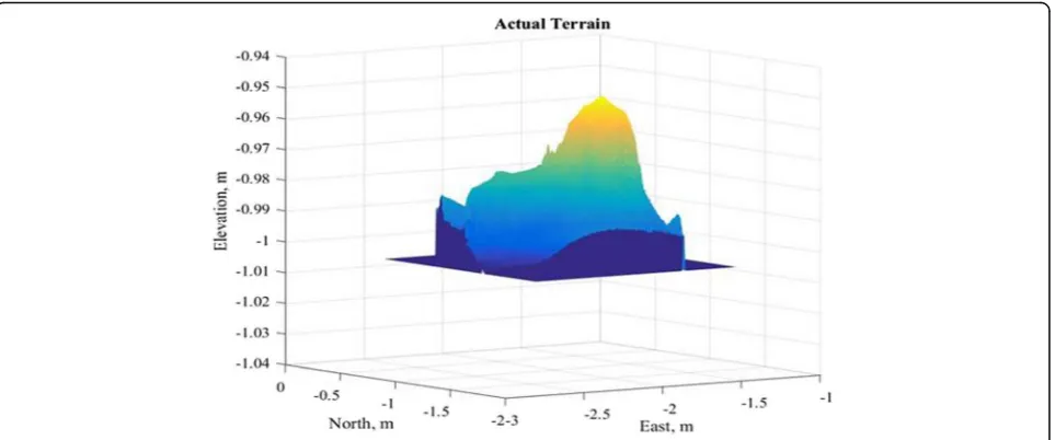
The uncertainty model and associated anchor points not only account for the spatial uncertainty, but also consider the function of time. A stochastic estimator traces the evolution of such randomness, in which the anchor points form a space of “states”. Thus, the eleva-tion and uncertainty of any given point at any time can be approximated with a combination of these states. In a software simulation, we created a landform of 150 by 150 m, and simulated the elevation change over the course of 30 years. Both the landform and the elevation change have non-linear surfaces (Fig. 1). To demonstrate the concept of using anchor points, we first formulated

a 5 by 5 array, which has sufficient density for a discre-tized representation of the simulated landform. However, anchor points do not necessarily form any regular shape in general.

Data from a TLS, an ALS, a 2D aerial camera, a stereo vision system, structure from motion SfM-MVS from a limited number of historic aerial photographs taken from a nadir-looking camera, static and Kinematic GNSS surveys are considered in our simulations (Table 1). These sensors differ greatly in accuracy and resolution. We assume all the sensor errors can be pro-jected onto the vertical direction, and thus only the ver-tical errors are of concern in developing an objective comparison among the various sensors.

Gaussian error models are used for GNSS positioning in this simulation. Naturally, the static surveys are more accurate. However, the Kinematic GNSS survey will gather more data points (Table 1).

The uncertainty in laser ranging measurements can be modeled with two main components, angular and radial. Although the complete ranging error model may be sophisticated (Thrun et al. 2005), it is often sufficient to assume that in practice, both error sources follow a normal distribution. The underlying mechanisms are in-dependent from each other (Glennie 2007). Figure 2 il-lustrates a typical application of laser scanner, which applies to both TLS and ALS. The laser scanner is ele-vated from the ground by h, and it scans a location on the ground at a line of sight distance r. Errors in the horizontal (azimuth) and vertical (elevation) angles re-sult from laser beam width and the precision in orienta-tion measurements and follow a 2D normal distribuorienta-tion (red ellipse in Fig. 2). Since the focus of this work is not on the high-fidelity simulation of ALS data, the compre-hensive error model (Glennie 2007) is abstracted and represented with two components: a radial errorσr, and

a vertical angular error σθ. A target observed at distance

rhas the total uncertainty ofσv. Compared to an ALS, a

TLS is closer to the ground, produces a denser point

cloud, and has more accurate ranging measurements. The ALS, on the other hand, scans the ground from a high altitude, in which case the vertical error is less sen-sitive to the angular uncertainty.

Data from a 2D camera image does not provide direct observation of elevation, as can be seen in Table 1. How-ever, 2D images can be related to the 3D landform via a 3D-2D projection model (Hartley and Zisserman 2003). Let vector [u,v]T represent the 2D location of a pointL on the image of a landform, observed using a camera with lens focal length f, and vector xC_L;y_LC;zC_LT be the 3D location of pointL, as observed in the camera frame (Cframe). The 3D-2D relationship can be modeled with

u v ¼zfC

L

xC L

yC L " #

;

which is implemented in the estimator. Any change in xC

L and yCL are thus observable in 2D images. The

land-form elevation change is observed on thezaxis in a Glo-bal frameG, ΔzG_L. As shown in Fig.3, pointLis located at XG_L, and it is being observed by a camera located at XG

C, both in the global frame. The elevation errorΔzGL is

related to the observation error made in the camera frame ΔxC_L. ΔxC_L can be geometrically decomposed into errors in the horizontal direction, ΔxG_L and the vertical direction, ΔzG_L in the global frame. The camera associ-ated with the aerial photography is typically locassoci-ated above the landform (Fig.3). The vertical observableΔzG_L is thus smaller than the horizontal component ΔxG_L in this geometry. Therefore, it tends to be less effective

(Table 1) when elevation changes are detected with an overhead image collected with an airborne camera.

The aforementioned projection model should not be confused with SfM-MVS, which operates on the same principle of multi-view geometry (Hartley and Zisserman 2003), as does stereo vision or triangulation. A camera in motion (with a limited overlapping nadir-looking im-ages to simulate a historic aerial photogrammetric ap-proach) will provide repeated observations of the same 3D landform [u,v]T1. . n, collected from n perspectives

(unstructured photographs). In this process, the camera orientation and location are known at allnperspectives, referenced to frame G. The 2D images, [u,v]T1. . n will

then be converted into unit vectors in frame G,UG1. . n.

At the ith perspective, UGi points from the camera

pos-ition XG_C;i to the landform position XG_L. Since XG_L does not change over the different perspectives, it is solved by using UG1. . n and XGC;1::n via an optimization process

(Hartley and Zisserman 2003). Figure 4 illustrates the geometric relationship between the landform and the camera on perspectives 1 and n. The uncertainty of XG_L will also be dependent on the accuracy of UG1. . n and

XG

C;1::n, and the geometric relationship between XGC;1::n

and XG_L. We conservatively assume a short displacement between camera perspectives in this experiment, which results in greater vertical errors in SfM.

The stochastic estimator uses measurements that be-come available sequentially over time. Let a state vector

xrepresent the vertical errors on the 25 anchors, located at mx[1..25], and a 25 by 25 matrix Pfor the covariance among states. x and P are initialized with some Table 1Sensor resolution and error

Sensor name TLS ALS 2D camera SfM Static GNSS Kinematic GNSS

Vertical error standard deviation in simulated data (m) 0.02 0.1 N/A 3.3 0.04 0.08

Sample Density (pt/km2) 1.1 × 107 7 × 103 1.1 × 105 1.1 × 105 278 2.2 × 104

The values presented herein are representative of our instrumentation and our experience to represent sensor quality. The large vertical error is observed with SfM since the displacement between camera perspectives is short in the simulation and is represented of legacy aerial photography. Sample density represents the density of measurements used to update the estimator in this simulation. It does not necessarily represent the density of raw data available from these sensors (such as TLS and ALS)

Fig. 2Laser scanner error model.θ: vertical angle,r: range,σr: standard deviation of radial ranging error,σθ: standard deviation of vertical angular

measurements, such as a TLS scan at timetk-1, and then

propagated to another timetkusing a Brownian process.

xk;k−1¼Fxk−1;k−1þμ

Pk;k−1¼FPk−1;k−1FþQ;

whereF is a matrix describing the dynamic relationship between states, which will be the identity matrix in this case. μ is the process noise component, corresponding to the Brownian process, of which the covariance matrix is defined withQ.

Without additional measurements, the matrix P, will grow as a function of time. The Brownian process may be established with the best-known model of terrain change, and will only be used to predict the increase of uncertainty if the model is valid for the underlying geo-morphic process.

The fundamental concept can be illustrated using just two of the anchor points, located atmx[1]andmx[2],

re-spectively. The initial uncertainty of both points can be represented with two circles att0(Fig. 5). As time

prop-agates to t1, the uncertainty grows for both points,

il-lustrated with greater circles. A new measurement becomes available at t1, made at location mz[t1]. The

uncertainty of this measurement is represented with an ellipse. This measurement is then used to update both anchor points. Right after this update, att1+, the

uncer-tainty of both points is reduced to ellipses. Since the update is closer to mx[2], the corresponding ellipse

be-comes smaller than that of mx[1]. Without additional

measurements, both ellipses are propagated tot2, which

result in greater ellipses. A second measurement was made at t2, which occurred much closer to mx[1] this

time. It effectively reduced the size of the ellipses, more so onmx[1]thanmx[2].

Fig. 32D camera image error model in a typical aerial photography application

The geometric relationship between anchor points and any measurement can still be represented or approxi-mated with a linear/linearized model, which can be established by using an interpolation method. Notice that the interpolation model used in this step estimates the covariance function, instead of predicting the land-form as does Kriging or polynomial regression. The bicu-bic interpolation method introduced in Keys (1981) has been widely used in the computer vision community, and it has been adopted in digital elevation surface modeling (Dumitru et al. 2013). With bicubic interpolation, a linear-ized relationship between a given point and the anchor points, denoted with matrix H, can be easily estimated. This approach handles non-linear landforms, and remains relatively computationally efficient.

The elevation at mz now has a direct measurement z, and a prediction from the estimator states, Hxk; k−1. Any disagreement between them is likely a result of un-certainties associated with both and new information that can be observed as“innovation”on the states,

y¼z−Hxk;k−1;

with a de-facto standard estimation method, the Kalman filter (Kalman1960),xandPare updated with a gainK:

K ¼Pk;k−1H′HPk;k−1H′þR−1

which allows us to update the states xand covarianceP using this new information:

xk;k ¼xk;k−1þKy

Pk;k¼ðI−KHÞPk;k−1

After this step, the states are further propagated onto

timet_{k + 1}, with the integration of another measurement

(such as aerial photo). The time history of states x and covariance matrix P are the outcome of this approach. Notice that only a few key steps of the estimator are highlighted here for the sake of conciseness. For details on the derivation and implementation, please refer to (Kalman 1960) and (Smith et al. 1962).

At any given point in time,x andPare used as input to predict the elevation and uncertainty of any given point on the landform with a standard interpolation method. An accurate and consistent covariance matrixP is the key to an optimum interpolation process. Consistency of covariance is defined based on how well

Pdescribes and over-bounds the actual error in statesx. To verify the estimation, x will be compared against a truth reference x_ref used in the software simulation. With field data, the truth reference can be generated from a high-resolution, high-fidelity sensor such as TLS. The variance and covariance of errorΔx=x−x_ref, is ex-pected to be closely bounded by Pat each time step t_k. Since it may be difficult to visualize the comparison be-tween matrices, the standard error σ_Δx[k] will be com-pared against an uncertainty level for this step, by using the root mean square of all the diagonal elements inP.

σest½ ¼k

ffiffiffiffiffiffiffiffiffiffiffiffiffiffiffiffiffiffiffiffiffiffi

diagPk;k q

In the software simulation, the actual elevation change is not provided to the estimator. Rather, an over-bounding Brownian process is used, and we expect to haveσest≥σΔxin the history of 30 years.

Physical modeling experiment

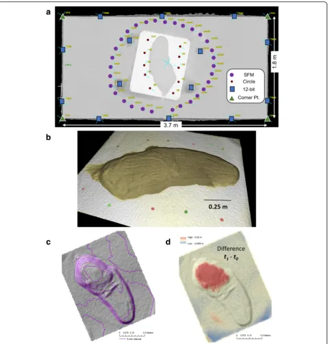
A physical model is developed in the Terrain Analysis Lab at East Carolina University as a further means of validating our uncertainty measures. The controlled simulation is designed around a fan-shaped surficial fea-tures (i.e. an alluvial fan or washover fan) built in a stainless-steel stream table (3.7 m long by 1.8 m wide) using coarse sand on a white sheet of plotter paper to reduce reflectivity of the stainless-steel table (Fig. 6). The fan-shaped feature is 0.974 m wide and 0.392 m in with a relief of 0.05 m from the bottom of the stream table (Fig. 6).

A Leica P20 laser scanner was inverted and mounted on an aluminum swing set (Lisenby et al. 2014). Targets mounted on the wall of the lab and within the stainless-steel table as well as the corner points of the table were used to register the TLS data (Fig. 6). Cartesian Fig. 5Two anchor points located mx[1](blue) and mx[2](red) show

what happens when new measurements become available over time. Uncertainty in both points are represented bycirclesand the

coordinates associated with TLS point clouds provide lo-cations for the control points used in the SfM. A single scan from the nadir looking position of the scanner cap-tured the entire simulated fan surface in t0and t1.SfM

data were collected with a Ricoh GR II digital camera. The camera was positioned at two different heights at 32 locations looking obliquely and inward at the fan surface (Fig. 6). A total of 64 images were used to generate a

point cloud with the aid of Agisoft Photoscan software. A combination of 14 12-bit targets from the Agisoft soft-ware were printed on sticky back paper and adhered to the stainless-steel table, along with 10 small circle tar-gets with known dimensions. Tartar-gets and circles were used to aid in the photo alignment process.

The original landform (t0) was modified (t1) by adding

the fan (Figs. 6 and 7) to emulate fan segment aggrad-ation over an arbitrary time-period (for example,t1is set

to 30 years). TLS and SfM-MVS data are collected at botht0andt1.TLS att1is used as a truth reference. We

initialize the estimator at t0 with TLS and SfM-MVS,

propagate and update at t1 using SfM-MVS. The

esti-matedσest½ 1 is compared against the actual errorσΔx[1]

in this case.

Results and discussion

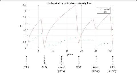
The estimator in the software simulation is initialized with a TLS scan. Subsequently, five additional sensor data sets become available over 30 years, to observe the geomorphic change. A general pattern evolves whereby the estimated uncertainty provides an over bound of the actual error (Fig. 8), i.e., σest≥σΔx. Both σest and σΔx

grow over time during the simulation, and are dramatic-ally reduced by some measurements, such as ALS, SfM-MVS and Kinematic GNSS surveys. Other sensors, such as 2D photos and static GNSS, are less effective, as ex-pected. Although the SfM-MVS measurements are not nearly as accurate as static GNSS survey, it offers a much higher point density and therefore, is also able to reduce the error more effectively. The over-bounding as-sociated with the static GNSS has more to do with the lack of data produced with this technique than the ac-curacy of the data collected. The truth reference used in this software simulation can be used to verify the estima-tion inx(Fig. 9).

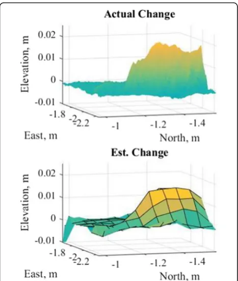
The estimator is also applied to the changes associated with the lab-simulated fan model. As this terrain is more sophisticated, a 20 by 20 mesh of anchors is used. The actual changexrefis obtained by comparing the two TLS scans (Fig. 10). The estimated change is observed on the

anchor points, by using a less accurate and lower-resolution SfM-MVS update. Att1= 30 years,σest ¼5:6

mm and σΔx= 3.7mm, σest is greater than, and yet rea-sonably close to σΔx. The difference is below the

detect-able limits for topographic change associated with the data source instrumentation (Wester et al. 2014, Staley et al. 2014; Wasklewicz and Scheinert 2015).

The software simulation and physical modeling experi-ment both show that the estimator can provide a reliable and consistent measure of uncertainty in legacy data. Al-though some sensors are more desired than others, the availability of sensors in legacy data and sometimes also in new data collection campaigns dictates that data from all sensors must be incorporated. The estimator will allow us to retrieve information from sensors of low ac-curacy, low observability (2D images) or low spatial resolution (static surveys). We further emphasize that the discussed estimator is not limited to just the Kalman filter. Other Bayesian estimators, such as particle filters (Montemerlo and Thrun 2003), are applicable as well. Similarly, bicubic interpolation is not the only choice for interpolation either. Other methods that can yield a line-arized relationship between measurements and states are also valid options, which will provide various types of advantages (Dumitru et al. 2013).

The statistical consistency of uncertainties in all the sensor measurements and estimates are critical in our application. In practice, repeated measurements could also lead to a covariance matrix P that is too small (Julier and Uhlmann 2001), such as high-density data from SfM-MVS. Asx and Pcan be used to predict the elevation and uncertainty of the whole landform, an overly optimisticPcan easily cause unexpected errors in the prediction. For instance, few erroneous points in x

with small variances would dominate the prediction and generate a bias in a neighborhood. Overly optimistic P also would prevent x from being updated with other sensors. Additional steps will be taken in future work to guarantee the consistency ofP.

The successful outcomes and corroboration in our ini-tial software and physical modeling simulations, the ability to adopt and use multiple estimators and interpolation techniques, and an ability to be employed across a variety of environmental settings provides a new alternative to in-tegrating legacy and HRT data.

Applications of existing and planned methodology to field research will help extend our understanding of the

dynamic landform and landscape changes that take place through space and time. At present, earth science re-searchers conducting studies with the aid of HRT data have placed a great deal of emphasis on methods and techniques that provide rapid, accurate, and spatially continuous topographic data. HRT provide the user with unparalleled information of short-term changes in pro-cesses and forms. Subtle topographic changes that earth scientists must measure in the future, for example those associated with climate change (Lane 2013), require de-tailed data that can be precisely acquired and accurately assessed to address scientific questions and inform pol-icy makers. However, the sole use of HRT data limits the Fig. 8Uncertainty of software simulated landform over 30 years, estimated sigmaσestvs. actual errorσΔx

temporal framework for which earth scientists can con-sider these changes because these data sets have only been recently developed. Legacy topographic data allow us to extend this temporal perspective of change back-ward in time to better inform us of variations on decadal time-scales and in some instances, as far back as a half-century or more (Corsini et al. 2009; Carley et al. 2012; James et al. 2012; Schaffrath et al. 2015). While we ap-preciate that this represents a miniscule amount of time from a geological perspective, the ability to use legacy topographic data increases the temporal sample size earth scientists are working from and allows us to make more authoritative statements about landform evolution than the shorter-term view supplied by research solely using HRT data.

Scientists need to be able to definitively measure the environmental changes and communicate these mea-sures to a broad audience of possible users that include their peers, public officials, and the community. Express-ing the uncertainty associated with these measurements or reducing the uncertainty in the data production process is a critical first step to achieving more definitive measures and communication. Here, our uncertainty model, associated anchor points, and stochastic estima-tor clearly highlight that spatial uncertainty can be accounted for across the time-scales of the legacy and HRT data. Each elevation point/grid has an associated

error, which can be used to produce better maps when interpolating to raster data and provide better measure-ment tolerances as they relate to topographic changes and sediment transport.

The ability to accurately assess spatially variable uncer-tainty across a broad range of temporal scales also pro-vides a means to exchange information between researchers, engineers, policy makers, and environmental managers and planners. The longer-term understanding of topographic change and sediment transport and the uncertainties associated with these dynamics permits greater understanding of issues such as: water quality, habitat loss, and risks to built-environments and human lives from environmental hazards. Furthermore, an ability to measure the level of data uncertainty associated with past landform and landscape dynamics will help advance landscape evolution models because of the ability to cor-roborate existing landscape evolutionary models with the longer-term record of topographic change derived from legacy topographic data sets and recent HRT data. This is a necessary advancement as we may come to rely on land-scape evolution models as an integral tool in the decision and management schemes as we face climate change and increased scenarios of extreme weather.

Conclusions

Our software simulation and physical modeling experi-ments provide a new approach to measuring topo-graphic data uncertainty where legacy data from a variety of data sources can be integrated with HRT data to expand the time-scales of topographic change detec-tion. As anticipated, the difference in the actual and ex-pected errors of our HRT physical model experiment was quite small (< 2 mm). Current instrumentation and field methods often have a higher minimal level of detec-tion, so this value is quite acceptable for HRT data sources and represents a value comparable to or lower than most uncertainty measures found in current research exploring topographic change detection. The uncertainty model, associated anchor points, and stochastic estimator was further applied to a software simulation whereby a variety of remote-sensing data sources were used to simu-late data capture from legacy data sources. Our findings show the estimated error coincides with the actual error using certain sensors (Kinematic GNSS, ALS, TLS, and SfM-MVS). Data from 2D imagery and static GNSS did not perform as well at the time the sensor is integrated into estimator. Nevertheless, the software simulation shows the approach can be used to estimate the error as-sociated with all elevation values in the legacy and HRT data over the time-period of the simulation.

Our findings show a strong potential for this tech-nique to be applied in a variety of field settings. We an-ticipate further development of the uncertainty model in Fig. 10Actual vs. estimated terrain change in lab-simulated fan

future research. Our goal is to expand the capability to densify the anchor points in areas that are more topo-graphically complex and test by overfitting the surface how well the uncertainty model is performing in these locations. At present, it is not clear if the use of sparse points (for example, techniques that rely on interpolation from topographic maps) under sample the topographic surface and therefore, do not accurately represent the sur-face or the spatially variable uncertainty in the measure-ment of topographic change. We intend to expand the capabilities of the model by conducting further software simulations that analyze and visualize topographic change over time using the varied densification of anchor points. The advances in the uncertainty model will then be fur-ther evaluated using real-world data from a variety of sources. For example, ALS data can be used in a fashion to simulate different types of data by varying the data density, data noise, etc. to examine known differences in the data and the capability to measures these data pertur-bations using the refine uncertainty model. Once these items have been worked out our intent is to apply the un-certainty model to the real-world topographic and envir-onmental changes within various envirenvir-onmental settings that include more topographically complex areas like mountainous environments versus less topographic com-plex locales such as barrier islands.

Our existing uncertainty model shows clear evidence that the temporal component of spatially variable uncer-tainty of legacy topographic data sets can be measured in both of our simulations. A capacity to integrate legacy topographic data expands earth scientist’s ability to understand topographic changes and sediment transport over longer time-scales. This should lead to more defini-tive measurements and answers regarding how environ-ments are changing over the past 50 to 100 years (dependent upon the temporal availability of topographic data sources). More conclusive measures and findings stem from our ability to assess uncertainty across the spectrum of legacy data in relation to more recent HRT data using techniques like we have documented in this research. New results from these approaches should pro-vide valuable information to the broader scientific com-munity and society. Societal benefits will likely be recognized in the form of delivering relevant informa-tion that show the potential range for environmental changes over time-scales demanded by managers and policy makers.

Abbreviations

ALS:Airborne laser scanning; DEM: Digital elevation model; DEM-of-difference; GNSS: Global navigation satellite system; HRT: High-resolution topography; SfM-MVS: Structure from Motion-Multi-View Stereo; SIE: Survey and interpolation error; TIN: Triangular irregular networks; TLS: Terrestrial laser scanning

Acknowledgements

We thank Kailey Adams and Robert Rankin for their assistance in our experiments.

Funding

This work was funded by an East Carolina University Interdisciplinary Research Collaboration Award entitled“Development of Scalable Sensor Payload for Rapid High Resolution Topographic Scanning via Micro Aerial Vehicles”. Funding for this award was supplied by the Division of Research and Graduate Studies in partnership with the Divisions of Academic Affairs and Health Sciences. The Terrain Analysis Lab and ECU Department of Geography, Planning, and Environment, provided the physical modeling facilities and equipment to simulate field measurements in a controlled setting.

Authors’contributions

TW proposed the topic, helped conceive the study design, analyzed the data, helped with the interpretation of the data, co-wrote the paper, and is corresponding author. ZZ helped conceive the study design, carried out the experimental study, analyzed the data, interpreted the data, designed figures, and co-wrote the paper. PG helped in the interpretation of the data and co-wrote the paper. All authors read and approved the final manuscript.

Competing interests

TW, ZZ, and PG declare that they have no competing interest.

Publisher’s Note

Springer Nature remains neutral with regard to jurisdictional claims in published maps and institutional affiliations.

Author details

1_{Department of Geography, Planning, and Environment, East Carolina}

University, Brewster Building A227, Greenville, NC 27858, USA.2College of Engineering and Technology, East Carolina University, Science and Technology Complex Suite 100, Greenville, NC 27858, USA.

Received: 28 January 2017 Accepted: 28 September 2017

References

Brasington J, Langham J, Rumsby B (2003) Methodological sensitivity of morphometric estimates of coarse fluvial sediment transport. Geomorphology 53:299–316 Brasington J, Rumsby BT, McVey RA (2000) Monitoring and modelling

morphological change in a braided gravel-bed river using high resolution GPS-based survey. Earth Surface Processes and Landforms 25: 973-990 Carley JK, Pasternack GB, Wyrick JR, Barker JR, Bratovich PM, Massa DA, Reedy GD,

Johnson TR (2012) Significant decadal channel change 58_–67 years post-dam accounting for uncertainty in topographic change detection between contour maps and point cloud models. Geomorphology 179:71–88

Corsini A, Borgatti L, Cervi F, Dahne A, Ronchetti F, Sterzai P (2009) Estimating mass-wasting processes in active earth slides_–earth flows with time-series of high-resolution DEMs from photogrammetry and airborne LiDAR. Nat Hazards Earth Syst Sci 9:433–439

Cortes J (2009) Distributed kriged Kalman filter for spatial estimation. IEEE Trans Autom Control 54:2816_–2827

Crowell M, Leatherman SP, Buckley MK (1991) Historical shoreline change: error analysis and mapping accuracy. Journal of coastal research, 839-852 Dumitru PD, Marin P, Dragos B (2013) Comparative study regarding the methods

of interpolation. In: Recent advances in geodesy and Geomatics engineering, pp 45–52

Elfe A (1989) Using occupancy grids for mobile robot perception and navigation. Computer 22:46–57

Fonstad MA, Dietrich JT, Courville BC, Jensen JL, Carbonneau PE (2013) Topographic structure from motion: a new development in photogrammetric measurement. Earth Surf Process Landf 38:421–430

Glennie C (2007) Rigorous 3D error analysis of kinematic scanning LIDAR systems. J Appl Geodesy 1:147_–157

Glennie CL, Hinojosa-Corona A, Nissen E, Kusari A, Oskin ME, Arrowsmith JR, Borsa A (2014) Optimization of legacy lidar data sets for measuring near-field earthquake displacements. Geophys Res Lett 41:3494–3501

Gomez C, Hayakawa Y, Obanawa H (2015) A study of Japanese landscapes using structure from motion derived DSMs and DEMs based on historical aerial photographs: new opportunities for vegetation monitoring and diachronic geomorphology. Geomorphology 242:11–20

Heritage GL, Milan DJ, Large AR, Fuller IC (2009) Influence of survey strategy and interpolation model on DEM quality. Geomorphology 112:334_–344 James LA, Hodgson ME, Ghoshal S, Latiolais MM (2012) Geomorphic change

detection using historic maps and DEM differencing: the temporal dimension of geospatial analysis. Geomorphology 137:181_–198

Julier SJ, Uhlmann JK (2001) General decentralized data fusion with covariance intersection (CI). In: Handbook of data fusion. CRC Press, Boca Raton Kalman RE (1960) A new approach to linear filtering and prediction problems.

J Basic Eng 82:35_–45

Keys R (1981) Cubic convolution interpolation for digital image processing. IEEE Trans Acoust Speech Signal Process 29:1153–1160

Krige DG (1951) A statistical approach to some mine valuations and allied problems at the witwatersrand. Master_’s thesis. University of Witwatersrand, Witwatersrand Lane SN (2013) 21st century climate change: where has all the geomorphology

gone? Earth Surf Process Landf 38:106–110

Lane SN, Westaway RM, Murray-Hicks D (2003) Estimation of erosion and deposition volumes in a large, gravel-bed, braided river using synoptic remote sensing. Earth Surf Process Landf 28:249–271

Lisenby PE, Slattery MC, Wasklewicz TA (2014) Morphological organization of a steep, tropical headwater stream: the aspect of channel bifurcation. Geomorphology 214:245–260

Mardia KV, Goodall C, Redfern EJ, Alonso FL (1998) The Kriged Kalman filter. TEST 7:217–285

Micheletti N, Lane SN, Chandler JH (2015) Application of archival aerial photogrammetry to quantify climate forcing of alpine landscapes. Photogramm Rec 30:143–165

Milan DJ, Heritage GL, Hetherington D (2007) Application of a 3D laser scanner in the assessment of erosion and deposition volumes and channel change in a proglacial river. Earth Surface Processes and Landforms 32:1657-1674 Milan DJ, Heritage GL, Large AR, Fuller IC (2011) Filtering spatial error from

DEMs: implications for morphological change estimation. Geomorphology, 125: 160-171

Montemerlo M, Thrun S (2003) Simultaneous localization and mapping with unknown data association using FastSLAM. Proceedings of IEEE International Conference on Robotics and Automation, Taipei

Oskin ME, Arrowsmith JR, Corona AH, Elliott AJ, Fletcher JM, Fielding EJ, Gold PO, Garcia JJG, Hudnut KW, Liu-Zeng J, Teran OJ (2012) Near-field deformation from the el mayor-Cucapah earthquake revealed by differential LIDAR. Science 335:702_–705

Pelletier JD, Brad Murray A, Pierce JL, Bierman PR, Breshears DD, Crosby BT, Ellis M, Foufoula-Georgiou E, Heimsath AM, Houser C., Lancaster, N (2015) Forecasting the response of Earth's surface to future climatic and land use changes: A review of methods and research needs. Earth's Future, 3(7)220-251 Schaffrath KR, Belmont P, Wheaton JM (2015) Landscape-scale geomorphic

change detection: quantifying spatially variable uncertainty and circumventing legacy data issues. Geomorphology 250:334–348 Smith GL, Schmidt SF, McGee LA (1962) Application of statistical filter theory to

the optimal estimation of position and velocity on board a circumlunar vehicle. National Aeronautics and Space Administration, Washington, D.C Spencer T, Naylor L, Lane S, Darby S, Macklin M, Magilligan F, Möller I (2017)

Stormy geomorphology: an introduction to the special issue. Earth Surf Process Landf 42:238–241

Staley DM, Wasklewicz TA, Kean JW (2014) Characterizing the primary material sources and dominant erosional processes for post-fire debris-flow initiation in a headwater basin using multi-temporal terrestrial laser scanning data. Geomorphology 214:324–338

Tarolli P, Sofia G (2016) Human topographic signatures and derived geomorphic processes across landscapes. Geomorphology 255:140_–161

Thrun S, Burgard W, Fox D (2005) Probabilistic robotics. MIT press, Boston Wasklewicz T, Scheinert C (2015) Development and maintenance of a

telescoping debris flow fan in response to human-induced fan surface channelization, Chalk Creek valley natural debris flow laboratory, Colorado, USA. Geomorphology 252:51–65

Wasklewicz T, Staley DM, Reavis K, Oguchi T (2013) Digital terrain modeling. In: Shroder J, Bishop MP (eds) Treatise on geomorphology, vol 3. Academic Press, San Diego, pp 130–161

Wasklewicz TA, Hattanji T (2009) High-resolution analysis of debris flow–Induced Channel changes in a headwater stream, Ashio Mountains, Japan. Prof Geogr 61:231–249

Wester T, Wasklewicz T, Staley D (2014) Functional and structural connectivity within a recently burned drainage basin. Geomorphology 206:362_–373 Wheaton JM, Brasington J, Darby SE, Sear DA (2010) Accounting for uncertainty

in DEMs from repeat topographic surveys: improved sediment budgets. Earth Surf Process Landf 35:136–156