R E S E A R C H
Open Access
Multiple imputation using chained equations for
missing data in TIMSS: a case study
Donia Smaali Bouhlila
*and Fethi Sellaouti
* Correspondence: [email protected] Université de Tunis El Manar, Faculté des Sciences Economiques et de Gestion de Tunis, Laboratoire Prosepective, Stratégies et Développement durable (PS2D), Tunis, Tunisia
Abstract
In this paper, we document a study that involved applying a multiple imputation technique with chained equations to data drawn from the 2007 iteration of the TIMSS database. More precisely, we imputed missing variables contained in the student background datafile for Tunisia (one of the TIMSS 2007 participating countries), by using Van Buuren, Boshuizen, and Knook’s (SM 18:681-694,1999) chained equations approach. We imputed the data in a way that was congenial with the analysis model. We also carried out different diagnostics in order to determine if the imputations were reasonable. Our analysis of multiply imputed data confirmed that the power of multiple imputation lies in obtaining smaller standard errors and narrower confidence intervals in addition to allowing one to work with the entire dataset.
Background
Missing data are a part of almost all research. Scrutiny of data from the iterations of TIMSS (Trends in International Mathematics and Science Study) makes clear that the survey participants, whether students, teachers, or school principals, fail to complete all of the items of their respective questionnaires. Because TIMSS data offer a rich array of information about the major factors thought to predict student achievement in mathematics and science, the incomplete cases mean not only a loss of power of the analyzed data but also the potential to bias the estimates of interest (Little, 1992; Little & Rubin, 2002).
Our aim in this paper is to apply the multiple imputation technique introduced by Rubin in the early 1970s (see Rubin, 1987) to a TIMSS dataset and thereby explore its possibility as a solution to the problem of survey nonresponse. We begin by examining the theoretical underpinnings of multiple imputation and then briefly describe
trad-itional imputation approaches. Next, we use Van Buuren, Boshuizen, and Knook’s
(1999) multiple imputation by chained equations approach to provide an illustration of imputing student background data missing from the TIMSS 2007 datafile for Tunisia.
Multiple imputation: a review of the literature
Among the traditional methods developed to enable investigators to make statistical inferences when data are incomplete are listwise deletion or complete case analysis, pairwise deletion, mean substitution, regression imputation, and inclusion of an indica-tor variable.aOver the last two decades, investigators have used these methods, despite
their drawbacks, extensively in their empirical research. The drawbacks include further loss of data, biasing the sample statistics, and reducing the variance of the variable in question (Acock, 2005; Little & Rubin, 2002; Peugh & Enders, 2004; Rubin, 1987).
More statistically principled methods for handling missing data also exist. They include the maximum likelihood estimation via the expectation maximization algorithm (EM) (Dempster, Laird, & Rubin 1977) and multiple imputation (Little & Rubin, 2002; Rubin, 1978, 1987, 1996; Schafer & Graham 2002). These methods produce estimates that are su-perior to those of the older methods, but for many researchers, multiple imputation is the general solution to missing-data problems in statistics (Rubin, 1996; Schafer, 1997). Cer-tainly, multiple imputation is an innovative approach over the traditional ones. On the one hand, researchers in many fields can use it. On the other hand, because its implemen-tation is becoming easier (thanks to the existence of statistical software packages), re-searchers are tempted to use it despite the problems associated with it.b
What is multiple imputation?
Before explaining what multiple imputation is, we consider it useful to study the mech-anisms and patterns associated with missing data.
Exploring missing-data mechanisms
The missing-data mechanism has three classifications (Rubin, 1976): missing at random (MAR), missing completely at random (MCAR), and missing not at random (MNAR). Data are said to be missing at random (MAR) if other variables in the dataset can be used to predict missingness on a given variable. For example, in surveys, men may be more likely than women to refuse to answer some questions. Here, data will be missing completely at random (MCAR) because the process that causes missingness does not depend on the values of variables in the dataset subject to analysis (Little, 1988; Rubin, 1976; Zhang, 2003).
MCAR is a fairly strong assumption, and tends to be relatively rare. For instance, in the context of survey data, MCAR data might occur when a respondent simply skips an item or a question, perhaps because of neglecting to turn the page of a question-naire booklet. MAR is a less restrictive assumption than MCAR. Finally, data are said to be missing not at random (i.e., MNAR, also called nonignorable missing data) if the value of the unobserved variable itself predicts missingness. A classic example of this is income. Individuals with very high incomes generally refuse to answer questions about their earnings. This is not the case for individuals with more modest incomes.c
Careful consideration of the missing-data mechanism is important because different types of missing data require different treatments (Allison, 2000; Schafer, 2003). When data are MCAR, the complete cases analysis will not result in biased parameter estimates. The only cost is a reduction in the sample size and the statistical power of the analysis be-cause MCAR leads to larger standard errors. In contrast, analyzing only complete cases for data that are either MAR or MNAR can lead to biased parameter estimates. Because multiple imputation generally assumes that the data are, at the least, MAR, this approach can also be used on data that are MCAR (Marchenko & Eddings, 2011).
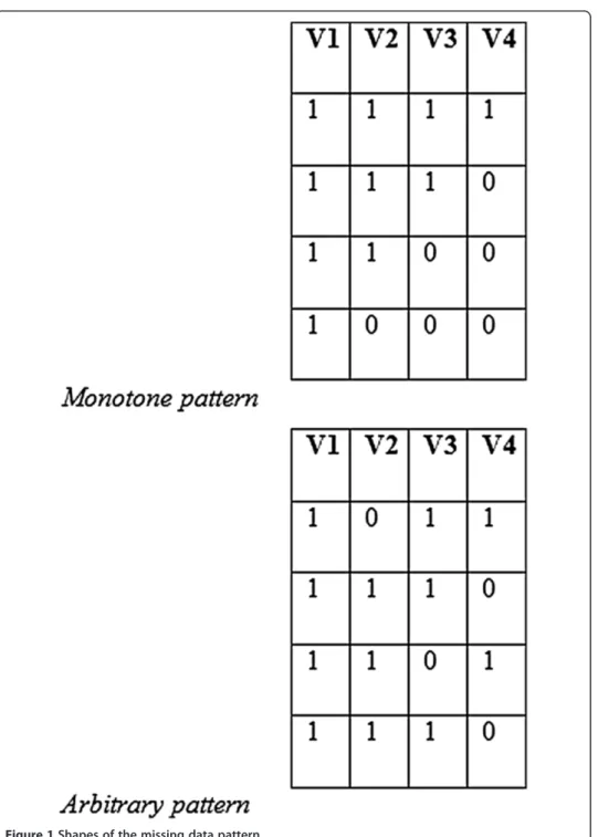
Exploring missing-data patterns
pattern. With a monotone pattern, X2 is observed only on a subset of subjects on
whom X1 is observed. X3is observed only for a subset of those on whom X2 is
ob-served, and so on (Raghunathan, Lepkowski, Van Hoewyk, & Solenberger, 2001). With the arbitrary pattern, missingness is widespread. Figure 1 provides an example of a monotone, arbitrary-patterned dataset containing four variables—V1to V4, where 1 s
indicate observed values and 0 s indicate missing values.
Monotone imputation requires a specific order of the prediction equations. X1is
im-puted using all of the complete variables as predictors, and X2is then imputed using
the observed and imputed values of X1and the other predictor variables. Thus, with
this process, the previously imputed variables are added sequentially to the prediction equations of the other imputation variables.d
Overview of multiple imputation
Multiple imputation is a statistical technique for handling incomplete data and for de-livering an analysis that makes use of all possible information (Rubin, 1977, 1978). It was derived using the Bayesian paradigm (Rubin 1987, 1996). Multiple imputations are repeated random draws from the predictive distribution of the missing values. More precisely, multiple imputations are drawn from a posterior predictive distribution of the missing data conditional on the observed data.
When seeking a Bayesian imputation model, we need to take all sources of variability and uncertainty in the imputed values into account in order to yield statistically valid inferences (Rubin, 1987). The process of substituting the predicted values for the
miss-ing ones is performed M times (M> 1). (We discuss choice of imputation models and
the number of imputations later in this paper.)
Imputing the missing data leads to the database, called the “imputed database”,
appearing to be complete, and allows researchers to apply complete-data-based
methods on each of the M imputed datasets. The parameter estimates, usually known
as the regression coefficients, are averaged using rules established by Rubin (1987) to produce a single set of results (see the Appendix to this paper). Multiple imputation thus requires the building of an imputation model in which predictor variables have to be specified. For discussions of the theoretical and statistical foundations of multiple imputation, see Nielsen (2003), Rubin (1987), and Zhang (2003).
Building an imputation model
In order to implement multiple imputation in practice, we first need to specify the pre-dictor variables. Having done that, we can then construct a predictive model.
Specification of the predictor variables The first task that needs to be accomplished when carrying out multiple imputation is selection of the predictor variables. We dis-cuss several approaches to determining which variables to include.
Meng (1994), Rubin (1996), Taylor et al. (2002), and White, Royston, and Wood (2011) advocate including all variables associated with the probability of missingness, along with the variables contained in the dataset. From a practical perspective, deciding which variables to include can be accomplished by establishing the correlations be-tween each variable to be imputed and the predictors. If the magnitude of a correlation exceeds a certain level, then the applicable variable is included (Van Buuren et al., 1999). Allison (2002), Moons, Donders, Stijnen, and Harrell (2006), and White et al. (2011) all highlight the need to include the dependent variable of the analysis model in the imputation model.
In the same spirit, and in order to have a rich imputation model compatible with the analysis model, Stuart, Azur, Frangakis, and Leaf (2009) argue for the necessity of in-cluding in the regression models those variables that lead to some minimum additional
R-squared. Another alternative is to use the variables that will be used in the analysis model in the imputation model (Schafer, 1997, Raghunathan et al., 2001). However, as Raghunathan and his colleagues (2001) have shown, the inclusion of more and more variables leads to the standard errors of the estimates for the analysis model becoming smaller and smaller.
Specification of the imputation modelcThe next step in multiple imputation is
speci-fication of the imputation model. Two distinct approaches are used—the multivariate
normal model and the chained equations approach.
Imputation using the multivariate normal model
The multivariate normal model was introduced by Rubin (1987; see also Little & Rubin 2002). This approach involves drawing from a multivariate normal distribution of all the variables in the imputation model, and it assumes that the variables are continuous and normally distributed. However, many datasets, especially those in international large-scale assessment databases, contain several different types of variable— categor-ical, binary, and skewed continuous. As such, the inclusion of nonnormally distributed variables in an imputation model that assumes normality may introduce bias. A prag-matic approach here is to transform these variables in order to obtain approximate nor-mality (Sterne et al., 2009; White et al., 2011).
Schafer (2001, p. 7) discusses several ways to manage nonnormally distributed vari-ables. For instance, he explains that nominal variables can be modeled in a way to ap-proximate normality, and the continuous imputed values can be rounded off to the required category. Skewed continuous variables can be transformed by standard func-tions such as the logarithm, the square root, or the reciprocal square root, and after im-putation transformed back to the original scale. Other variables with problematic distributions can be transformed by a method based on the empirical cumulative distri-bution function.
Shafer (2001) used this imputation model to impute the NHANES III dataset after modeling nonnormally distributed variables. Peugh and Enders (2004) demonstrated the use of multiple imputation using the multivariate normal model in the context of the Longitudinal Study of American Youth. Enders et al. (2006) also used this approach to impute missing data in the Longitudinal Study of Adolescents at Risk for the
Devel-opment of Emotional or Behavioral Disorders. Schafer’s (1999b) NORM program was
used to conduct all of these illustrative analyses.e
One drawback of imputing variables by assuming normality is that the distribution of the imputed values may not resemble that of the observed values (White et al., 2011). Although this approach has stronger theoretical underpinnings and some better statis-tical properties, the chained equations approach works well in practice (Raghunathan
et al., 2001; Van Buuren et al., 1999; Van Buuren, Brand, Groothuis–Oudshoorn, &
Imputation using the chained equations approachg
This approach is sometimes referred to as ICE or MICE (i.e., multiple imputation by chained equations). It is also known as the fully conditional specification and sequential regression multivariate imputation (White et al., 2011). MICE is a practical approach for imputing missing datasets based on a set of imputation models, given that there is one model for each variable with missing values. MICE has been described in the con-text of medical research conducted by Royston and White (2011), Van Buuren et al. (1999), and White et al. (2011), and it is seen as a suitable approach for imputing in-complete large, national, public datasets. Work conducted by Oudshoorn, Van Buuren, and Van Rijckevorsel (1999) provides an illustration of this approach. They used MICE to obtain a complete version of the Dutch National Services and Amenities Utilization Survey of 1995 (AVO-95). The MICE procedure requires development of the MICE al-gorithm, a description of which follows.
Because the ICE approach involves a series of univariate models rather than a single large model, the MICE approach imputes data on a variable by variable basis by speci-fying an imputation model per variable. Suppose we have a set of variables X1……Xk.
Of this set of variables, some or all have missing values. If X1has missing values, it will
be regressed on the other variables X2to Xk. The estimation is thus restricted to
indi-viduals with observed X1. The missing values in X1are then replaced by the predictive
values, which are simulated draws from the posterior predictive distribution of X1. The
following variable with missing values, X2, is regressed on all the other variables X1, X3
to Xk. Estimation is thus restricted to individuals with observed X2and uses the
im-puted values of X1. Here again, the missing values in X2 are replaced by simulated
draws from the posterior predictive distribution of X2.
This process is repeated for all the other variables in turn for n cycles in order to stabilize the results and to produce single imputed datasets. Royston and White (2011) and Van Buuren et al. (1999) have all suggested that more than 10 cycles are needed for the convergence of the sampling distribution of imputed values, whereas the entire
procedure is repeated independentlyMtimes, yieldingMimputed datasets.
Selecting the number of imputations
It is important to know the number of imputations needed for a good statistical
infer-ence. Multiple imputation theorists suggest that small values of M, on the order of
three to five imputations, yield excellent results (Rubin, 1987; Schafer & Olsen, 1998). Schafer (1999a) suggests that no more than 10 imputations are usually required. Graham, Olchowski, and Gilreath (2007) recommend that researchers using multiple imputation should perform many more imputations than previously considered suffi-cient. They reached this conclusion after using a Monte Carlo simulation to test multiple-imputation models across several scenarios in which the fraction of missing
informationhfor the parameter being estimated andMwere varied.
White et al. (2011) offer another argument in favor of increasing M. Their approach
is based on calculating the Monte Carlo error of the results, with the latter defined as the standard deviation across repeated runs of the same imputation procedure with the
same data. White and his colleagues showed, using UK700 data,i that Monte Carlo
thumb, although they qualified it as not universally appropriate, which states that M
should be at least equal to the percentage of incomplete cases in the dataset. If, for
ex-ample, 70% of cases have complete data, this rule would suggestM= 30.
Imputation models for different types of variables
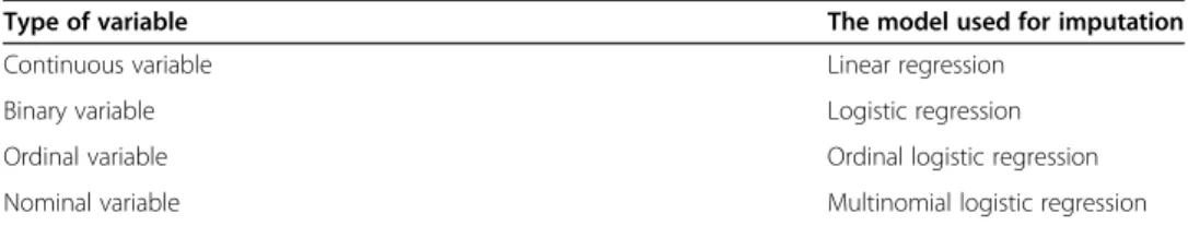
In general, datasets contain several types of variables that do not necessarily follow a normal distribution. An interesting feature of MICE is that it can handle different vari-able types (continuous, binary, unordered categorical, ordered categorical) by building different MICE algorithms (Royston & White 2011; White et al., 2011). Table 1 sets out the models that are used for different types of variable. Sometimes, continuous vari-ables are either positively or negatively skewed. White et al. (2011) discuss two main ways of dealing with such variables: transformation towards normality and predictive mean matching.
Advantages of MICE and comparison of it with the multivariate normal model (MVN) Despite lacking a theoretical rationale and despite the difficulties encountered when specifying the different imputation models, MICE has several practical advantages (Marchenko, 2011; Van Buuren et al., 2006; Van Buuren & Oudshoorn, 2011; White et al., 2011). The particularly interesting feature of MICE is its flexibility: each variable can be modeled by using a model tailored to its distribution. In addition, MICE can manage imputation of variables defined only on a subset of the data (e.g., pregnant women). MICE can also incorporate variables that are functions of other variables, and it does not require monotone missing-data patterns.
Brief mention of a number of comparisons between MICE and MVN is relevant here (see, in particular, Lee & Carlin, 2010; Marchenko, 2011; Van Buuren, 2007). To begin with, the multivariate normal model has theoretical underpinnings whereas MICE does not. Secondly, MICE imputes data on a variable by variable basis, but MVN uses a joint modeling approach based on a multivariate normal distribution (Schafer, 1997). MICE can also handle different types of variables while the variables imputed under MVN need to be normally distributed or transformed in order to approximate normality (Schafer, 1997). Finally, MICE can include restrictions within a subset of the data, whereas MVN imputation cannot.
Methods
Implementing MICE in the TIMSS datafile for students’background: a case study
Since their launch in the 1960s by the International Association for the Evaluation of Educational Achievement (IEA), international large-scale assessments such as
Table 1 Imputation models for different types of variables
Type of variable The model used for imputation
Continuous variable Linear regression
Binary variable Logistic regression
Ordinal variable Ordinal logistic regression
the Trends in Mathematics and Science Study (TIMSS) and the Progress in Inter-national Reading Literacy Study (PIRLS) have become increasingly attractive to
countries wanting to assess their students’ achievement in mathematics, science,
and reading literacy. IEA studies focus on student achievement and the factors re-lated to it. They provide high-quality data for evidence-based educational policy and reform.
TIMSS was first conducted in 1994/1995, in 45 countries, at five grade levels (3, 4, 7, and 8, and the final year of secondary school). The second assessment, conducted in 1999, involved 38 countries and surveyed only one grade, Grade 8. The third iteration, in 2003, assessed students in Grades 4 and 8 in 50 countries. Fifty-nine countries par-ticipated in the fourth survey, in 2007. The students tested this time round were fourth and eighth graders. Just over 60 countries took part in the fifth and most recent TIMSS survey, conducted in 2011 and again surveying fourth and eighth graders. A number of these countries today have at hand data spanning over two decades, that is, from 1995 to 2011. The next TIMSS survey is scheduled for 2015.j
The central aim of TIMSS is to assess students’ achievements in mathematics and
science. Another equally important purpose is to produce data that allow investigators
to explore and identify factors relating to student learning, such as students’ home
backgrounds, as well as other factors arising out of policy changes relating to, for ex-ample, curricular emphases, allocation of resources, and instructional practices. These dual purposes are accomplished by administering questionnaires to participating stu-dents, their mathematics and science teachers, and the principals of the sampled schools.
The TIMSS assessments use a two-stage, clustered sampling design. During Stage 1, school selection is based on a probability proportional to size sampling approach, whereby there is a higher probability of choosing larger schools. The second stage con-sists of randomly choosing one or two intact classes at Grade 8 level. All students in the selected classes are then assessed, except for students excluded for specified reasons (e.g., intellectual disability) and students absent on the day of assessment. TIMSS also employs school stratification in order to improve the efficiency of the sample design. Both explicit and implicit stratifications are used. However, even in the absence of stratification, the TIMSS samples represent, on average, the different groups found in the wider population (Olson, Martin, & Mullis, 2007, p. 84).
TIMSS researchers use sampling weights to accommodate the fact that the probabil-ities associated with selecting some units, such as schools, teachers, and students, will differ. It is therefore necessary to consider the purpose of analysis when choosing sam-pling weights (Rutkowski, Gonzalez, Joncas, & Von Davier, 2010; Schafer, 2001). The inclusion of weights for each individual imputation makes it easier to ensure that the imputation model is appropriate (Rubin, 1996). Our advice regarding imputation of missing data is to use thetotal student weightwhen imputing missing values in the
stu-dent datafile, to use the weight for mathematics/science teacher data when imputing
missing values in the mathematics/science teacher file, and to use school weight when
imputing nonresponse in the school datafile.
and the failure of individuals to provide information. “Omitted”, “not administered”, and “don’t know responses” are all considered to be missing values and hence in need of imputation.
Omitted responses:These occur when a student, teacher, or school principal skips a question. Invalid answers in the background questionnaires, such as when the respondent selects two or more response options in a categorical variable, are considered to be omitted and thus missing (Foy & Olson,2007).
Not administered:The not administered code is used in the TIMSS background questionnaire datafiles when a respondent fails to complete a questionnaire or when a question is not administered because of, for example, having been left out, misprinted, removed from the questionnaire, considered not applicable in some countries,k mistranslated, or deemed not internationally comparable (Foy & Olson,2007).
Don’t know responses:As Little and Rubin (2002) point out, deciding what to do with individuals who respond with“don’t know”is especially challenging. The don’t know response occurs in questions that, for example, ask students about the highest education level of either parent or about the level of education they themselves expect to complete. In order to consider this subpopulation as part of the population under study, we need to tag the don’t know response as missing and therefore requiring imputation.
Types of variables in TIMSS
TIMSS datafiles contain different variable types: continuous, binary, nominal, and or-dinal. Continuous variables are those that have an infinite number of possible values, such as age, plausible values in mathematics and in science, minutes spent teaching mathematics per week to a class, and total school enrollment. Binary variables are nom-inal variables that have two categories, for example, gender, whether or not students were born in the participating country, and possessions at home, such as a calculator.
Nominal variables are those that have more than two categories, such as whether or not the students’ parents were born in the participating country. Finally, ordinal vari-ables, although similar to nominal varivari-ables, differ from the latter because the variables are clearly ordered. Examples of ordinal variables include the highest level of education attained by either parent and the amount of time the student spends watching televi-sion or video within a specified time period (e.g., weekly). Rating scales is another cat-egory of variables that can be considered ordinal. They include the customary four-or five-point Likert scale variables of, for example, strongly disagree, disagree, agree, or strongly agree (with a statement or proposition).
Illustrative analysis
So far we have mainly discussed the approaches used to generate multiply imputed datasets. We have also addressed how MICE could potentially be used in relation to TIMSS background files. In this section, we focus on implementing MICE to missing values of variables contained in the files encompassing background data from the
stu-dents who participated in TIMSS in Tunisia.lWe begin by defining our analysis model.
this by assessing the missing data in order to determine their pattern and the“ mechan-ism”producing that pattern. We also discuss the different diagnostics we used to deter-mine whether the imputations were reasonable or whether the procedure needed to be modified. Finally, we present our analysis of the multiply imputed data.
The analysis model
We decided to apply our MICE approach to a study examining the relationship be-tween mathematics performance and science performance of the Grade 8 Tunisian
stu-dents as well as their socioeconomic status and their respective schools’ resources.
Since the Coleman report of 1966 (Coleman et al., 1966), an extensive body of
litera-ture has built up that explores and identifies the factors associated with students’
achievement in developing and developed countries.
Socioeconomic status and school resources are the variables most discussed in the lit-erature. We therefore decided that our analysis model should be as follows:
Tics¼α0þα1Ficsþα2Rcsþεics:
Here, Tics is the first plausible value in mathematics (or in science) provided by
TIMSS 2007.Ficsreflects the socioeconomic status of the studentiin classcand school s, and ε is the error term that has a school-level element and a class-level element in addition to the individual-student element (Moulton, 1986).Rcsis the index of
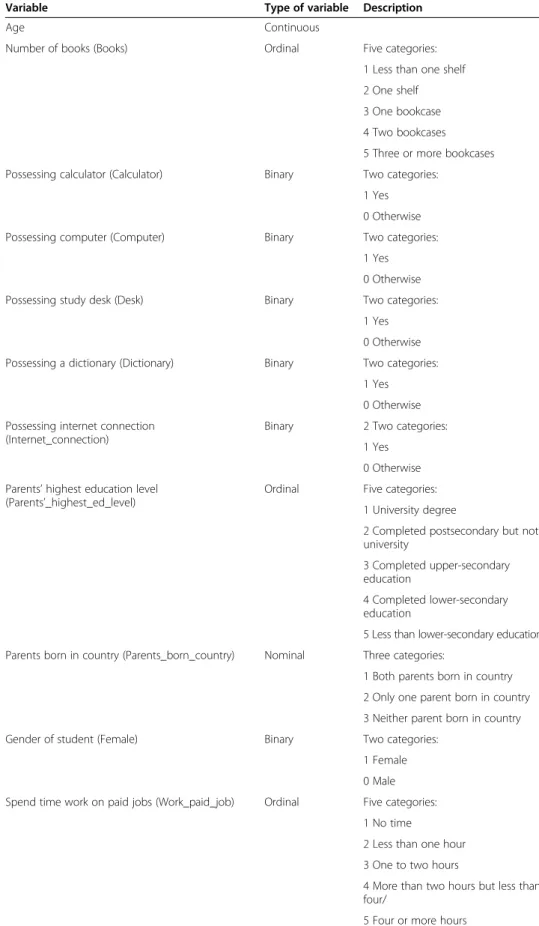
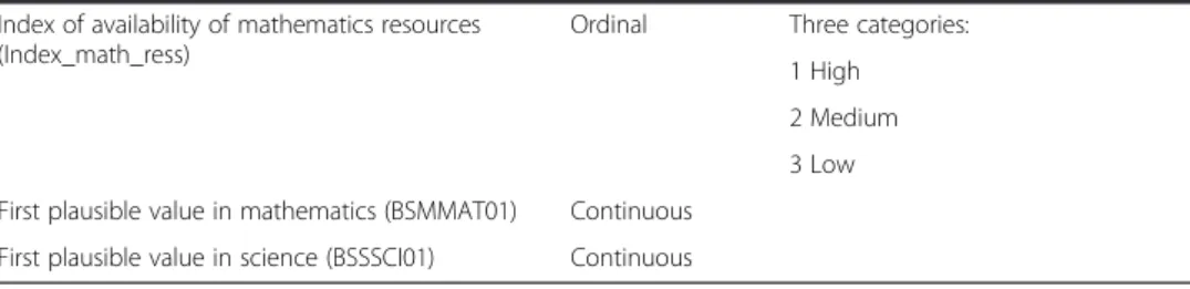
availabil-ity of school resources for mathematics instruction in class c at schools. Table 2 de-scribes the variables used in our analysis. We included all of these variables in our imputation model.
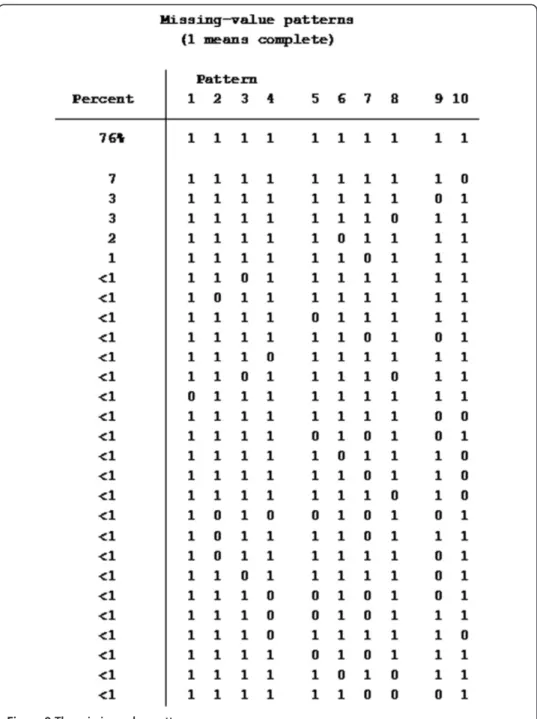
Assessing missing data
This step can be accomplished by examining the pattern of missing data as well as ex-ploring the missing-data mechanism. Scrutiny of our data revealed an arbitrary missing pattern, as can be seen in the Appendix (Figure 9) to this paper. Sample statistics indi-cated that only 76% of observations were complete; the remaining 24% of the data thus contained missing values. The output of the misstable nested presented immediately below clearly shows that the missing values of the different variables were not nested because 10 statements describe the missing value pattern, thereby confirming the arbi-trary nature of the missing data pattern (see Misstable nested).
Misstable nested
1. Index_math_ress (23) 2. Calculator (70)
3. Parents_born_country (77) 4. Desk (78)
5. Dictionary (84) 6. Books (109)
7. Internet_connection (172) 8. Work_paid_job (180) 9. Computer (240)
Table 2 Description of the different variables
Variable Type of variable Description
Age Continuous
Number of books (Books) Ordinal Five categories:
1 Less than one shelf
2 One shelf
3 One bookcase
4 Two bookcases
5 Three or more bookcases
Possessing calculator (Calculator) Binary Two categories:
1 Yes
0 Otherwise
Possessing computer (Computer) Binary Two categories:
1 Yes
0 Otherwise
Possessing study desk (Desk) Binary Two categories:
1 Yes
0 Otherwise
Possessing a dictionary (Dictionary) Binary Two categories:
1 Yes
0 Otherwise
Possessing internet connection (Internet_connection)
Binary 2 Two categories:
1 Yes
0 Otherwise
Parents’highest education level (Parents’_highest_ed_level)
Ordinal Five categories:
1 University degree
2 Completed postsecondary but not university
3 Completed upper-secondary education
4 Completed lower-secondary education
5 Less than lower-secondary education
Parents born in country (Parents_born_country) Nominal Three categories:
1 Both parents born in country
2 Only one parent born in country
3 Neither parent born in country
Gender of student (Female) Binary Two categories:
1 Female
0 Male
Spend time work on paid jobs (Work_paid_job) Ordinal Five categories:
1 No time
2 Less than one hour
3 One to two hours
4 More than two hours but less than four/
It is pertinent to note at this point that imputation using chained equations does not require the variables to be imputed in a specific order. The prediction models do not follow a specific order because, by default, the software imputes variables from the most observed to the least observed.
Having determined the pattern of missingness, we next needed to determine the mechanism driving it. The reason for this step relates to the fact that multiple imput-ation relies on certain assumptions. One assumption is that the data are MAR. How-ever, the missingness at random assumption is not testable. Nevertheless, we can test
the assumption of MCARm data against MAR data (Marchenko & Eddings, 2011a) by,
for example, creating a new dummy variable for each existing variable, which takes the value of 1 if a given observation is missing that variable and of 0 if it is not.
The next step is to run a logistic regression analysis, with the missing data dummy as the dependent variable, over the number of completely observed variables. If the ob-served variables predict missingness, then the data are MAR rather than MCAR. Fur-thermore, if there are no strong associations between missingness and the observed values, then the data are MCAR rather than MAR (Marchenko & Eddings, 2011). Our data showed no strong associations between missingness and the observed values, so
we assumed that the data were MCAR.n
Multiple imputation diagnostics
Imputation techniques require some diagnostics to help determine whether or not the imputations are reasonable. Recent research by a number of investigators has led to the development of important diagnostics that can be utilized before and after the im-putation process (Abayomi, Gelman, & Levy, 2008; Carpenter & Kenward, 2008; Gra-ham, 2009; Marchenko & Eddings, 2011; Raghunathan & Bondarenko, 2007; Stuart et al., 2009; Su, Gelman, Hill, & Yajima, White et al., 2011; 2011; Van Buuren & Oudshoorn, 2011).
Testing individual models before imputing A strength of MICE is that it allows modeling of each variable via a model tailored to its distribution. A good imputation model depends on the success of all the individual models. If a single model fails to converge, the imputation process as a whole fails. Checking the imputation models en-compasses the following steps:
1. Checking for convergence: The imputation model must run successfully.
Sometimes, complex models such as mlogit fail to converge if the number of Table 2 Description of the different variables(Continued)
Index of availability of mathematics resources (Index_math_ress)
Ordinal Three categories:
1 High
2 Medium
3 Low
First plausible value in mathematics (BSMMAT01) Continuous
categorical variables used is large. The reason why is because the large number can lead to small cell sizes. Pinning down the cause of the problem requires dropping some variables and then added them in, in small groups, until the model runs successfully. Although this method is time consuming, it does result in a workable model. Another alternative is to study the correlations between the nominal variable to be imputed and the predictors, and to choose only those that correlate significantly with the variable in question.
2. Handling problems of perfect prediction: Checking the model is a crucial step in the process of detecting perfect prediction. Perfect prediction occurs in regression models for categorical outcomes. Such models include logistic, ordered logistic, and multinomial logistic. Perfect prediction occurs whenever the outcome of any predictor variable within a category is always 0 (or always 1). It usually leads to infinite coefficients with infinite standard errors, and it often causes instability during estimation.
When endeavoring to resolve this problem, we have two options, one of which consists of discarding the variables responsible for perfect prediction. However, by doing this, we may defeat the whole purpose of multiple imputation, unless we have no intention of using the variables in further analyses. The second option is to handle perfect prediction directly during imputation via the augment option. This option, suggested by White, Daniel, and Royston (2010), is available for all categorical imputation methods (logit, ologit, and mlogit), and it allows us to add to the data extra observations with small weights during estimation of model parameters so that no prediction is perfect (White et al., 2010). For further details of this approach, see the section titled “The Issue of Perfect Prediction During Imputation of Categorical Data” in the STATA 12 multiple imputation documentation provided by the software STATA 12.
3. Adding interaction terms:Sometimes, imputing on subsamples is required for two reasons. The first is to ensure we have at hand the correct functional form of the imputation model, and the second is to preserve higher-order dependencies (Collins, Schafer, & Kam, 2001; Rubin, 1996; Schafer, 2001). For instance, we can investigate various interaction effects with respect to gender, race, income, age, and location (i.e., urban/rural). Thus, one way to check for misspecification is to add these interaction terms to the models in order to determine if they are important (Graham,2009). However, we cannot include a large number of interactions in the imputation models because of computational limitations (Stuart et al.,2009). Also, in“clustered data”, the members of the same cluster can share characteristics. In this situation, we can includethe cluster variable (either the strata or the primary sampling units) in the imputation model as an indicator variable (Graham,2009).
Imputation process and convergence check We used MICE to draw five multiple imputations per missing value,oand repeated the process through 100 cycles. As is clear from the output below, we successfully imputed all the incomplete values (Figure 2).
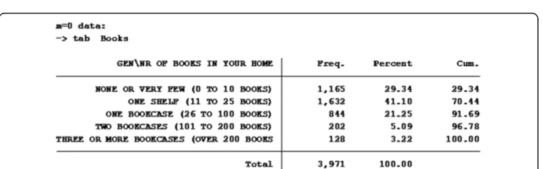
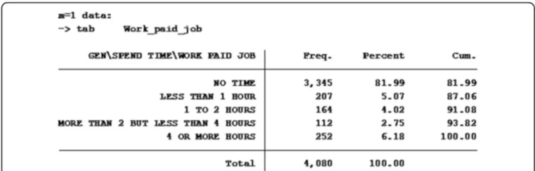
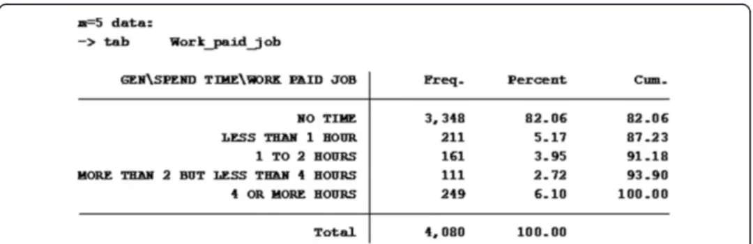
Our next step involved using frequency tables to check if the imputed data of the cat-egorical variables fitted the observed variable.p The frequency tables that follow are from the first and the last imputation (m= 1 andm= 5), as well as from the observed data (m= 0) of some of the selected variables. Note that the observed and the imputed values are relatively similar (Figures 3, 4, 5, 6, 7 and 8).
Results
Figure 2Imputation of the incomplete values.
datasets. After that, we performed 30 imputations and reanalyzed the estimation results, all of which appear in the Appendix (Figures 11, 12, 13, 14, 15, 16 and 17) to this paper.
As we mentioned earlier, our goal was to study the impact of SES variables and
school resources on students’ performance in mathematics and science. Although our
analysis was conducted over the first plausible values in mathematics and the first plausible value in science, we report here only the results of the first plausible value in
mathematics because the difference between the two results was minor.q The listwise
deletion of the original data is reported in Figure 11 in the Appendix.
We next generated five imputed datasets (Figure 12 in the Appendix) running the analyses separately on each dataset, and combining, by using Rubin’s (1987) rules, the
parameter estimates and standard errors into a single inference.r The resulting
esti-mates accounted for both within- and between-imputation uncertainty, reflecting the fact that the imputed values were not observed values.
On looking at Figure 12 we observe first that the multiple imputation estimates are quite similar to those obtained from the complete case analysis. However, after imputation, we can see that the standard errors are smaller and the confidence intervals narrower. Three statistics require interpretation at this point. They are the average relative variance increase (RVI), the largest fraction of missing information (FMI), and the degrees of freedom (DF).s
The average relative variance increase (RVI) due to nonresponse is small: 0.0407. It indi-cates the increase in variance of the estimates because of the missing values: the closer the number is to zero, the less effect missing data have on the variance of the estimate. The largest fraction of missing information (FMI), also called the rate of missing informa-tion (Graham et al., 2007; Schafer, 2001; Schafer & Olsen, 1998), reports the largest of all the FMI on coefficient estimates due to missingness. This statistic is particularly relevant because it lets us know whether or not the standard errors are affected by the variability of the imputed values across (in our case) the five datasets (Schafer, 2001).
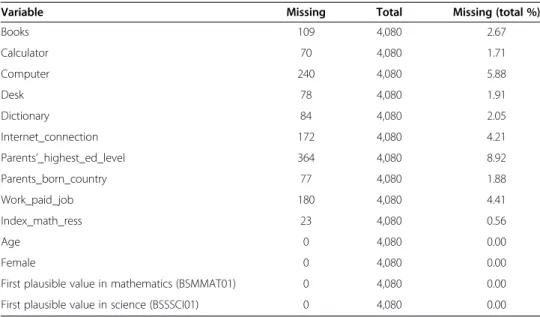
When comparing the estimated FMI (see Figure 14) to the percentage of missing data (Table 3), we can see that the estimated percentage rate of missing information is sub-stantially lower than the actual percentage of the imputed values (or missing data). This outcome tells us that the imputation procedure is making effective use of other infor-mation to predict the missing data (Schafer, 2001).
We can also use FMI to judge if the number of imputations is sufficient or not for analysis (White et al., 2011). A rule of thumb with respect to FMI is that the number of imputations M > = 100*FMI. In our case, FMI was 0.1565 and the number of imputa-tions was five. Therefore, according to this rule, we need to increase M.
As shown in Figure 13 degrees of freedom (DF) could be obtained for each coefficient. Averaging out at 131.99, the degrees of freedom are large. The reason is that multiple imputation degrees of freedom not only depend on the number of imputations but also inversely relate to the RVI. Also, and again as evident in Figure 13 the degrees of freedom were obtained under a small sample-assumption adjustment, which was determined by the type of reference distribution used for inference. The model F test assumes that the fractions of missing information of all coefficients are equal (equal FMI) and thus rejects the hypothesis that all coefficients are equal to zero.
Finally, we used the Taylor linearization variance estimation method to compute the variance estimates in each completed data analysis. Here we can see, in Figure 13 that the smallest degrees of freedom correspond to the coefficient for parents’_highest_ed_level
(2, 3, 4, and 5) (parents’highest attained level of education) because it contains the highest share of missing values. The largest degrees of freedom can be observed for the coefficient age, indicating that the loss of information due to nonresponse is the smallest for this coefficient. Figure 13 also displays, as a percentage, the increase in
Figure 6The frequency table of the variableWork_paid_jobfrom the observed data.
standard errors of the parameters due to missingness. Apparent is the increase from 0.03% (though negligible) to 8.20% in the standard errors for the coefficients.
In order to provide information about the variance specific to each parameter, Figure 14 displays the within-imputation variance and the between-imputation variance (see Rubin’s rules in the Appendix). It also sets out RVI, FMI specific to each parameter, and the relative efficiency of the overall imputation, which can be also used as an approximation when en-deavoring to determine the number of imputations (Graham et al., 2007; White et al., 2011). What we notice first in Figure 14 is that the between-imputation variability is very small relative to the within-imputation variability. The second aspect of interest is that
ageand femalehave the smallest within-imputation and between-imputation variances.
As expected, parents’ highest level of education has the highest RVI and FMI. The
reported relative efficiencies are high for all the coefficient estimates, suggesting the need to increase the number of imputations. These estimates are useful in indicating whether or not we should increase the number of imputations. However, we could also compute the Monte Carlo errors (MCE) of the estimates in order to help us reach this determination (White et al., 2011).
We accordingly again conducted the regression over the five imputed datasets involv-ing the computation of the MCE. White et al. (2011) suggest the followinvolv-ing guidelines for determining an acceptable amount of MCE:
1. The Monte Carlo error of a coefficient should be less than or equal to 10% of its standard error.
2. The Monte Carlo error of a coefficient’sT-statistic should be less than or equal to 0.1. 3. The Monte Carlo error of a coefficient’sP-value should be less than or equal to
0.01 if the trueP-value is 0.05, or 0.02 if the trueP-value is 0.1.
A look at the estimates in Figure 15 makes clear that these guidelines were not met for the following variables: computer, internet-connection, work on paid job (2, 3, and 4), and parents’_highest_ed_level(2, 3, 4 and 5). Increasing the number of imputations therefore seemed necessary.
In our example, 24% of the data were missing. Given the recommendation by White et al. (2011) that the number of imputations should be at least equal to the percentage of incomplete cases, we decided to perform 30 imputations. Figure 16 displays the re-sults of this stage of our analysis.tWe can see that the Monte Carlo errors now satisfy the guidelines. In addition, the estimates are quite similar to those obtained from the
complete case analysis: the standard errors are smaller (Figure 17), and the confidence intervals are narrower. Increasing the number of imputations has thus led to more pre-cision in computing thep-values, standard errors, confidence intervals, and fractions of missing information (Bodner, 2008).
Discussion
In this paper, we have described and evaluated the MICE procedure that can be used to impute missing values of different categories of variables. Although this approach lacks formal theoretical justification, it has the strong advantage of flexibility. Presumably, MICE can be used for TIMSS missing-data problems, given that most variables with miss-ing data in the TIMSS background datafiles are not normally distributed.
The difficulty in implementing MICE lies in the choice of predictor variables and interaction terms. To avoid bias and gain precision, researchers recommend that the
imputation models contain—at the least—every variable included in the analysis
model. However, the inclusion of interaction terms is a tedious process. A way to determine an interaction is to think of one of the variables as a grouping variable, such as gender (Graham, 2009), and then to carry out separate imputations for females and males.
Another matter associated with implementation of MICE is the issue of weights. TIMSS datafiles contain different kinds of weights, so before imputing the missing data we need to ask ourselves this question: Which weight should I use? As Rutkowski et al. (2010) point out, choice of weights depends on the purpose of the analysis and the re-search question. The inclusion of weights for each individual imputation makes it easier to ensure that the imputation model is appropriate. The appropriate weight to use
when imputing students’missing data is total studentweight. The weight to use when
imputing missing values in the mathematics teacher file is the weight for themathematics teacher data, and the one to use for nonresponse in the school datafile is the school
weight.
Table 3 Number and percentage of missing data
Variable Missing Total Missing (total %)
Books 109 4,080 2.67
Calculator 70 4,080 1.71
Computer 240 4,080 5.88
Desk 78 4,080 1.91
Dictionary 84 4,080 2.05
Internet_connection 172 4,080 4.21
Parents’_highest_ed_level 364 4,080 8.92
Parents_born_country 77 4,080 1.88
Work_paid_job 180 4,080 4.41
Index_math_ress 23 4,080 0.56
Age 0 4,080 0.00
Female 0 4,080 0.00
First plausible value in mathematics (BSMMAT01) 0 4,080 0.00
In general, careful modeling is required when using MICE to obtain valid statistical in-ferences (Marchenko, 2011). Another important point to remember concerns the order in which the imputation models should be imputed. Imputation using chained equations does not require us to specifically order the variables that must be imputed because the software imputes, by default, the variables from the most observed to the least observed.
In this paper, we also focused on the diagnostics of multiple imputation. The object-ive of this procedure is to identify those imputations that markedly differ from the ob-served values and then to pin down the cause of the problem. This process should determine if the imputation model should be remodeled or tested, for example, by means of sensitivity analyses, if there is a serious violation of the missingness assumptions. Also, because MICE is an iterative imputation method, its convergence needs to be evaluated.
Deciding on the number of imputations to conduct (especially if the number is likely to exceed the number theoretically considered sufficient—i.e., 5 to 10) is most easily done by computing FMI, the relative efficiency, or Monte Carlo errors (MCE). Studies show that computing MCE is a particularly suitable way of determining the number of imputations. When establishing the fraction of missingness, we can impute almost any fraction of missing data, provided that we do the imputation correctly and do not vio-late the assumption of MAR. However, if the fraction of missing data is large, say in the order of 30% to 50%, imputation methods must be applied with great caution (White et al., 2011).
In our illustrative analysis, we applied MICE to the student background data in the TIMSS 2007 datafile for Tunisia. We included all the variables used for imputation in the analysis model, and then performed five imputations, followed by another 30 impu-tations, after which we compared the results with the complete case analysis. The re-sults showed that the estimates were relatively similar to those obtained from the complete case analysis. However, after imputation, the standard errors were smaller and the confidence intervals narrower.
Conclusion
In this paper, we reviewed two approaches to multiple imputation—the multivariate nor-mal model and the chained equations approach. Multiple imputation is becoming easier and more tempting to use thanks to the existence of different software packages. It is re-ceiving growing attention from researchers in various fields, some of whom consider it to be“the-state-of-the art”missing-data technique (Schafer & Graham, 2002, p. 173) be-cause it provides unbiased parameter estimates, does not reduce the variance of the vari-able in question, and preserves the entire dataset. The outcomes of our application of MICE to TIMSS data exhibiting nonresponse suggest that empirical research can be conducted effectively with whole datasets, thereby leading to more accurate conclusions about the information contained not only in the TIMSS databases but also in the data-bases of other large-scale educational studies and surveys.
Endnotes
a
b
Different software packages are available to implement the multiple imputation technique. See, for instance, Acock (2005), Horton and Kleinman (2007), and Mayer, Muche, and Hohl (2012).
c
http://www.ats.ucla.edu/stat/stata/seminars/missing_data/mi_in_stata_pt1.htm (IDRE, 2013a).
d
See STATA 12 documentation.
e
This program can be downloaded free of charge at http://sites.stat.psu.edu/~jls/ misoftwa.html. NORM offers the user a number of normalizing transformations that can be implemented prior to the implementation phase and variables can be restored to their original metrics prior to analysis.
f
See also Van Buuren and Oudshoorn (2011) for a list of studies in which MICE has been used.
g
http://www.ats.ucla.edu/stat/stata/seminars/missing_data/mi_in_stata_pt2.htm (IDRE, 2013b).
h
This quantity figures prominently in multiple imputation. Also called the rate of miss-ing information, it differs from the percentage of missmiss-ing data. See Graham et al. (2007) and Schafer and Olsen (1998) for its formula and more discussion on it.
i
The UK700 data was a multi-center study conducted in four inner-city areas. Partic-ipants were between the ages of 18 and 65, had a diagnosed psychotic illness, and expe-rienced two or more psychiatric hospital admissions, the most recent within the previous two years. See White et al. (2011).
j
See the TIMSS website: timss.bc.edu.
k
Check whether the question is applicable or not to the country under study. If it is not applicable, then it cannot be considered as missing and should be removed from the analysis model.
l
Recently, Reiter and Si (2013) applied a different methodology (a fully Bayesian joint modeling approach) to impute missing background TIMSS 2007 data. They claim this ap-proach offers advantages over MICE because it can capture complex dependencies and be applied effectively to nonresponse within large-scale assessments.
m
It is also possible to test whether the MCAR assumption is plausible by using the multivariate test proposed by Little (1988).
n
Because testing the assumption of MAR against MNAR is impossible, it is always necessary to think about how the data being analyzed were collected (Marchenko & Eddings, 2011; Stuart et al., 2009).
o
It took roughly one hour to draw five multiple imputations.
p
The convergence of imputed continuous variables can be assessed using trace plots (see Marchenko, 2011).
q
Science results can be provided upon request from the authors.
r
See the Appendix to this paper.
s
We also referred to STATA 12 documentation when discussing the output.
t
It took us roughly six hours to draw 30 imputations.
Appendix A) Rubin’s rules
Let Q^1…::Q^M be the parameter estimates of Qobtained fromM imputed datasets. Combine these parameter estimates into a single point estimate by taking the arith-metic average of the parameter across theManalyses as follows:
Q¼ 1 M
X
i¼1
M
^
Qi:
The standard errors combine in a similar way. Note, however, that they require the calculation of two components: the within-imputation variance and the between-imputation variance. The within-between-imputation variance is computed by taking the arith-metic average of theMsquared standard errors as follows:
Q¼ 1 M
X
i¼1
M
^
Ui:
where, U^i is the squared standard error from the ithdataset. The between-imputation
variance is the variance of the parameter estimate itself across the M imputations:
B¼ 1 M
X
i¼1
M
^
Qi−Q
2
:
The total variance is:
T ¼U þ 1þ 1
M
B:
The overall standard error is:
S:E¼
ffiffiffiffiffiffiffiffiffiffiffiffiffiffiffiffiffiffiffiffiffiffiffiffiffiffiffiffiffiffiffiffiffi
Uþ 1þ 1
M
B s
:
A significance test of the null hypothesisQ= 0 is performed by comparing the ratio
t¼S:EQ to the samet-distribution. B) the missing data pattern
Competing interests
The authors declare that they have no competing interests.
Acknowledgement
We would like to acknowledge the helpful and constructive comments of the three anonymous reviewers of this paper.
Received: 28 August 2013 Accepted: 3 September 2013 Published: 16 September 2013
References
Abayomi, K, Gelman, A, & Levy, M. (2008). Diagnostics for multivariate imputations.Applied Statistics, 57(Series C, Part 3), 273–291.
Acock, AC. (2005). Working with missing data.Journal of Marriage and Family, 67(4), 1012–1028.
Allison, PD. (2000). Multiple imputation for missing data: a cautionary tale.Sociological Methods and Research, 28, 301–309.
Allison, PD. (2002).Missing data. Thousand Oaks, CA: Sage.
Bodner, TE. (2008). What improves with increased missing data imputations?Structural Equation Modeling, 15, 651–675. Carpenter, J, & Kenward, M. (2008).Brief comments on computational issues with multiple imputation. Unpublished paper
retrieved from http://missingdata.lshtm.ac.uk/downloads/mi_comp_issues.pdf.
Coleman, JS, Campbell, E, Hobson, C, McPartland, J, Mood, A, Weinfield, F, & York, R. (1966).Equality of educational opportunity. Washington, DC: US Government Printing Office.
Collins, LM, Schafer, JL, & Kam, CM. (2001). A comparison of inclusive and restrictive strategies in modern missing data procedures.Psychological Methods, 6(4), 330–351.
Dempster, AP, Laird, NM, & Rubin, DB. (1977). Maximum likelihood from incomplete data via the EM algorithm.Journal of the Royal Statistical Society: Series B: Methodological, 39(1), 1–38.
Enders, C, Dietz, S, Montague, M, & Dixon, J. (2006). Modern alternatives for dealing with missing data in special education research.Advances in Learning and Behavioral Disabilities, 19, 105–133.
Foy, P, & Olson, JF (Eds.). (2007).TIMSS 2007 international database and user guide. Chestnut Hill, MA: Boston College. Graham, JW. (2009). Missing data analysis: making it work in the real world.Annual Review of Psychology, 60, 549–576. Graham, JW, Olchowski, AE, & Gilreath, TD. (2007). How many imputations are really needed? Some practical
clarifications of multiple imputation theory.Prevention Science, 8, 206–213.
Horton, NJ, & Kleinman, KP. (2007). Much ado about nothing: a comparison of missing data methods and software to fit incomplete data regression models.The American Statistician, 61(1), 79–90.
Institute for Digital Research and Education (IDRE). (2013a).Statistical computing seminars: multiple imputation in Stata, part 1. Los Angeles, CA: IDRE, University of California at Los Angeles. Retrieved from http://www.ats.ucla.edu/stat/ stata/seminars/missing_data/mi_in_stata_pt2.htm.
Institute for Digital Research and Education (IDRE). (2013b).Statistical computing seminars: multiple imputation in Stata, part 2. Los Angeles, CA: IDRE, University of California at Los Angeles. Retrieved from http://www.ats.ucla.edu/stat/ stata/seminars/missing_data/mi_in_stata_pt2.htm.
Jolani, S, Van Buuren, S, & Frank, LE. (2011). Combining the complete-data and nonresponse models for drawing imputations under MAR.Journal of Statistical Computation and Simulation, 1, 1–12. doi:10.1080/
00949655.2011.639773.
Lee, KJ, & Carlin, JB. (2010). Multiple imputation for missing data: fully conditional specification versus multivariate normal imputation.American Journal of Epidemiology, 171(5), 624–632.
Little, RJA. (1988). A test of missing completely at random for multivariate data with missing values.Journal of the American Statistical Association, 83(404), 1198–1202.
Little, RJA. (1992). Regression with missing X’s: a review.Journal of the American Statistical Association, 87(420), 1227–1237.
Little, RJA, & Rubin, DB. (2002).Statistical analysis with missing data. Hoboken, NJ: Wiley.
Marchenko, YV. (2011).Chained equations and more in multiple imputation in Stata. Paper presented at the 2011 Italian Stata Users Group Meeting. Retrieved from http://www.stata.com/meeting/italy11/abstracts/italy11_marchenko.pdf. Marchenko, YV, & Eddings, WD. (2011).A note on how to perform multiple-imputation diagnostics in Stata. College
Station, TX: StataCorp. Retrieved from http://www.stata.com/users/ymarchenko/midiagnote.pdf.
Mayer, B, Muche, R, & Hohl, K. (2012). Software for the handling and imputation of missing data: an overview.Clinical Trials, 2(1), 1–8. Available online at http://www.omicsgroup.org/journals/JCTR/JCTR-2-103.php?aid=3766. Meng, XL. (1994). Multiple imputation inferences with uncongenial sources of input.Statistical Science, 9(4), 538–558. Moons, KG, Donders, RA, Stijnen, T, & Harrell, FE, Jr. (2006). Using the outcome for imputation of missing predictor
values was preferred.Journal of Clinical Epidemiology, 59, 1092–1101.
Moulton, BR. (1986). Random group effects and the precision of regression estimates.Journal of Econometrics, 32(3), 385–397.
Nielsen, SF. (2003). Proper and improper multiple imputation.International Statistical Review, 71(3), 593–607. Olson, JF, Martin, MO, & Mullis, IVS (Eds.). (2007).TIMSS 2007 technical report. Chestnut Hill, MA: Boston College. Oudshoorn, CGM, Van Buuren, S, & Rijckevorsel, V. (1999).Flexible multiple imputation by chained equations of the
AVO-95 survey (TNO Report PG/VGZ/99.045). Leiden, the Netherlands: TNO Prevention and Health.
Peugh, JL, & Enders, CK. (2004). Missing data in educational research: a review of reporting practices and suggestions for improvement.Review of Educational Research, 74(4), 525–556.
Raghunathan, TE, & Bondarenko, I. (2007).Diagnostics for multiple imputations. Available on the Social Science Research Network website: http://papers.ssrn.com/sol3/papers.cfm?abstract_id=1031750.
Reiter, JP, & Si, Y. (2013).Nonparametric Bayesian multiple imputation for incomplete categorical variables in large-scale assessment surveys. Unpublished paper retrieved from http://www.stat.duke.edu/~jerry/Papers/jebs12.pdf. Royston, P, & White, IR. (2011). Multiple imputation by chained equations (MICE): implementation in Stata.Journal of
Statistical Software, 45(4), 1–20.
Rubin, DB. (1976). Inference and missing data.Biometrika, 63, 581–592.
Rubin, DB. (1977). Formalizing subjective notions about the effect of nonrespondents in sample surveys.Journal of the American Statistical Association, 72, 538–543.
Rubin, DB. (1978). Multiple imputations in sample surveys-a phenomenological Bayesian approach to nonrepsonse.
Proceedings of the Survey Research Methods Section of the American Statistical Association, 20–34. Rubin, DB. (1987).Multiple imputation for non-response in surveys. New York, NY: John Wiley.
Rubin, DB. (1996). Multiple imputation after 18+ years.Journal of the American Statistical Association, 91, 473–489. Rutkowski, L, Gonzalez, E, Joncas, M, & Von Davier, M. (2010). International large-scale assessment data: Issues in
secondary analysis and reporting.Educational Researcher, 39(2), 142–151.
Schafer, JL. (1997).Analysis of incomplete multivariate data. New York, NY: Chapman and Hall. Schafer, JL. (1999a). Multiple imputation: a primer.Statistical Methods in Medical Research, 8, 3–15.
Schafer, JL. (1999b).NORM: Multiple imputation of incomplete multivariate data under a normal model [computer software]. University Park, PA: Department of Statistics, Pennsylvania State University.
Schafer, JL. (2001).Analyzing the NHANES III multiply imputed data set: methods and examples prepared for the national center for health statistics. Hyattsville, MD: National Center for Health Statistics.
Schafer, JL. (2003). Multiple imputation in multivariate problems when the imputation and analysis models differ.
Statistica Neerlandica, 57(1), 19–35.
Schafer, JL, & Graham, JW. (2002). Missing data: our view of the state of the art.Psychological Methods, 7(2), 147–177. Schafer, JL, & Olsen, MK. (1998). Multiple imputation for multivariate missing data problems: a data analyst’s perspective.
Multivariate Behavioral Research, 33, 545–571.
Sterne, JAC, White, IR, Carlin, JB, Spratt, M, Royston, P, Kenward, MG, Wood, AM, & Carpenter, JR. (2009). Multiple imputation for missing data in epidemiological and clinical research: potential and pitfalls.British Medical Journal, 339, 157–160.
Stuart, EA, Azur, M, Frangakis, C, & Leaf, P. (2009). Multiple imputation with large data sets: a case study of the children’s mental health initiative.American Journal of Epidemiology, 169(9), 1133–1139.
Su, YS, Gelman, A, Hill, J, & Yajima, M. (2011). Multiple imputation with diagnostics (mi) in R: opening windows into the black box.Journal of Statistical Software, 45(2), 1–13.
Taylor, JMG, Cooper, KL, Wei, JT, Sarma, RV, Raghunathan, TE, & Heeringa, SG. (2002). Use of multiple imputation to correct for non-response bias in a survey of urologic symptoms among African-American men.American Journal of Epidemiology, 156, 774–782.
Van Buuren, S. (2007). Multiple imputation of discrete and continuous data by fully conditional specification.Statistical Methods in Medical Research, 16(3), 219–242.
Van Buuren, S, & Oudshoorn, KG. (2011). Mice: Multivariate imputation by chained equations in R.Journal of Statistical Software, 45(3), 1–67.
Van Buuren, S, Boshuizen, HC, & Knook, DL. (1999). Multiple imputation of missing blood pressure covariates in survival analysis.Statistics in Medicine, 18, 681–694.
Van Buuren, S, Brand, JPL, Groothuis-Oudshoorn, CGM, & Rubin, DB. (2006). Fully conditional specification in multivariate imputation.Journal of Statistical Computation and Simulation, 76, 1049–1064.
White, IR, Daniel, R, & Royston, P. (2010). Avoiding bias due to perfect prediction in multiple imputation of incomplete categorical variables.Computational Statistics and Data Analysis, 54, 2267–2275.
White, IR, Royston, P, & Wood, AM. (2011). Multiple imputation using chained equations: Issues and guidance for practice.Statistics in Medicine, 30, 377–399.
Zhang, P. (2003). Multiple imputation: theory and method.International Statistical Review, 71(3), 581–592.
doi:10.1186/2196-0739-1-4
Cite this article as:Bouhlila and Sellaouti:Multiple imputation using chained equations for missing data in TIMSS: a case study.Large-scale Assessments in Education20131:4.
Submit your manuscript to a
journal and benefi t from:
7Convenient online submission
7Rigorous peer review
7Immediate publication on acceptance
7Open access: articles freely available online
7High visibility within the fi eld
7Retaining the copyright to your article