NUMERICAL ANALYSIS OF ELECTRO-HYDRAULIC FORMING PROCESS, BY USING VOLUMEACCELERATION LOADING

43

NUMERICAL ANALYSIS OF ELECTRO-HYDRAULIC

FORMING PROCESS, BY USING

VOLUMEACCELERATION LOADING

*Mehdi Zohoor, **Mansur Hosseini *Associate Professor, Faculty of Mechanical Engineering,

K. N. Toosi University of Technology, Tehran, Iran

**M.Sc. Student, Faculty of Mechanical Engineering, K. N. Toosi University of Technology, Tehran, Iran

ABSTRACT

Electro-hydraulic forming is one of the unique processes of high-velocity forming. In this process, the electrical energy is converted into the mechanical energy in the form of shock waves within a liquid medium. This energy is utilized to perform redundant work, to overcome the friction, and to form the work-piece to the final shape. This process is very similar to the explosive forming and the only difference is the source of energy. In this article, electrical discharge phenomenon was analyzed and the parameters involved in electro-hydraulic forming process were investigated. Then, the simulation of the process was performed using finite-element approach. In this research, three types of sheet metals were used which are mild steel (IF210), high strength steel (DPX800) and stainless steel (1.4509). In this simulation, a dynamic explicit analysis was adopted and the effect of electrical discharge was simulated both in the form of acoustic pressure loading and acoustic inward volume acceleration loading. Three-dimensional analysis was employed using a shell model as a sheet metal. The Johnson-Cook constitutive model was used to describe the plastic behavior of the material. Then, the geometry of the formed part and the strain distributions were evaluated.Finally, the results obtained from simulation were compared with the experimental results reported by other scientists and found a good correlation between them.

Keywords:High velocity forming, Electro-hydraulic forming, Finite element method, Electrical discharge, Johnson-cook

INTRODUCTION

44

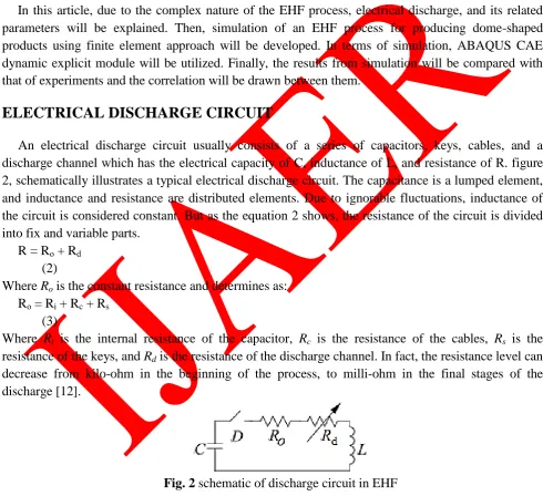
propagating towards the work-piece. Thus, the sheet moves into the die cavity and reaches its desired shape. Carrying the force by the liquid medium, the need for a punch is revoked. Compared with electro-magnetic forming, this process can form versatile metals due to its non-sensitivity to conduction.

A capacitor bank is utilized to store the energy needed. If the work-piece being formed is large and its thickness is considerable, the use of larger bank is mandatory. Electro-hydraulic forming process lasts fewer than 200 micro-seconds and the forming velocity reaches to amount of 300 metre per second [1]. Equation (1), computes the amount of energy accumulated in a capacitor bank.

𝐸_𝐶 =1

2𝐶𝑉

2

(1)

Where Ec is the energy stored in the capacitor (j), C is the electrical capacity (Farad), and V is the

voltage difference (volt).

Fig. 1 schematic of electro-hydraulic machine

In 1940, EHF was recognized as a potential method for forming of various parts. Until 1953, there were no reports regarding the utilization of EHF method. Afterwards, Early and Dow reported an under-water electrical discharge to form a part [3]. In the early 1950s, preliminary developments were achieved by Yutkin [4]. Bruno [5], Davies and Austin [6] investigated the applications of the EHF approach. Balanethiram et al. [7] conducted a survey on EHF processes and the results showed an enhanced forming limit comparing to traditional processes.

45

Finally a good correlation between simulations and experiments were obtained. Farzin and Montazerolghaem [11] also formed miniature products by EHF processes and by simulating in ABAQUS CAE, they investigated the effect of element size and time intervals in corner-filling of the die cavity.

SCOPE

In this article, due to the complex nature of the EHF process, electrical discharge, and its related parameters will be explained. Then, simulation of an EHF process for producing dome-shaped products using finite element approach will be developed. In terms of simulation, ABAQUS CAE dynamic explicit module will be utilized. Finally, the results from simulation will be compared with that of experiments and the correlation will be drawn between them.

ELECTRICAL DISCHARGE CIRCUIT

An electrical discharge circuit usually consists of a series of capacitors, keys, cables, and a discharge channel which has the electrical capacity of C, inductance of L, and resistance of R. figure 2, schematically illustrates a typical electrical discharge circuit. The capacitance is a lumped element, and inductance and resistance are distributed elements. Due to ignorable fluctuations, inductance of the circuit is considered constant. But as the equation 2 shows, the resistance of the circuit is divided into fix and variable parts.

R = Rο + Rd

(2)

Where Rο is the constant resistance and determines as:

Rο = Ri + Rc + Rs

(3)

Where Ri is the internal resistance of the capacitor, Rc is the resistance of the cables, Rs is the

resistance of the keys, and Rd is the resistance of the discharge channel. In fact, the resistance level can

decrease from kilo-ohm in the beginning of the process, to milli-ohm in the final stages of the discharge [12].

Fig. 2 schematic of discharge circuit in EHF

46 𝑑2𝑖

𝑑𝑡2+ 𝑅 𝐿

𝑑𝑖

𝑑𝑡 +

1 𝐿𝐶𝑖 = 0

(4)

Considering the preliminary conditions of:

𝑖 ∘ =∘, 𝑑𝑖

𝑑𝑡|𝑡=∘= −

𝑉∘ 𝐿

And by solving the differential equation 4, current-time and voltage-time functions can be obtained [13]. Electrical power of the discharge channel is described as follows:

𝑁 𝑡 = 𝑖(𝑡)𝑉(𝑡) (5)

Where 𝑖 𝑡 and 𝑉(𝑡) are the current and voltage respectively. The energy released in the channel is determined as follows:

𝐸_𝑑 𝑡 = 𝑁(𝑡)𝑑𝑡_°𝑡 (6)

Where t is the duration of plasma phase in the channel. All the energy is not transferred into the channel and the wire and keys prevent the whole energy to discharge. Thus the circuit efficiency should be taken into account:

𝜂_𝑑 = 𝐸𝑑 𝐸𝐶

(7)

Ed is the energy of the channel and Ec is the energy stored in the capacitor bank.

ELECTRICAL DISCHARGE ENERGY

If the water is exposed to a high-voltage DC pulse, an avalanche of electrons will be generated nearby the anode and this leads the water to ionize. Electrons then accelerate towards cathode in the presence of the electrical field. So the plasma channel initiates. Temperature rises up to 10000 Kelvin [12]. By initiating the plasma channel, the water evaporates and expands quickly. This, creates shock waves.

Different types of energies will be generated in the discharging moment. These include internal energy, radiation energy, shock wave energy and the bubble energy [12].

Ed=Ein+Era+Es+Eb

(8)

Ein, Era, Es and Eb are the internal energy, radiation energy, shock-wave energy and the bubble energy

respectively.

INTERNAL ENERGY

47

hydrogen and oxygen. According to Landau-lifshitz Law, a particle or ion within plasma channel can react in one of these 5 forms:

2H2O⥩2H2+O2 [+4.96 eV]

H2⥩2H [+4.48 eV]

O2⥩2O [+5.11 eV]

H⥩H++e- [+13.6 eV] O⥩O++e- [+13.6 eV]

Information inside the bracket corresponds the minimum energy required to initiate reaction. Thus the energy added to the channel is determined by the equation 9:

𝐸_𝑖𝑛 = 𝐸_{𝑖 𝑖} (9)

Ei is the energy added during each reaction.

RADIATION ENERGY

Thermal radiation depends on the temperature of the system and this phenomenon is described by Stefan-Boltzmann Law [12].

𝐸_𝑟𝑎 = 4𝜋𝑟_°2𝑆𝑡

(10)

Where ro is the radius of the channel, S is the electro-magnetic flux normal to channel area.

SHOCK-WAVE AND BUBBLE ENERGY

While electrical discharging beneath the water, shock-wave and bubble wave propagates through the medium. On account of the fact that the maximum pressure obtained from electrical discharge is reversely proportional with radial distance from the channel, the shock-wave energy is determined as follows:

𝐸𝑠 = 4𝜋 𝑟2𝑝 𝑡 𝑢(𝑡)𝑑𝑡 𝜏

0

(11)

Where u, the particle velocity is: 𝑢(𝑡) =𝑝(𝑡)

𝑐𝜌 . By substituting the u(t) in the equation above, the

shock-wave energy can be determined as follows [12 and 14]:

𝐸_𝑠 =4𝜋∙𝑟2

𝜌𝑐 𝑝

2_{(𝑡)𝑑𝑡} 𝜏

0

(12)

Where r is the distance from the source, ρ is the density of water, c is sound speed, τ is the width of shock-wave signal, and p(t) is the shock-wave pressure signal. The bubble wave energy is calculated by the equation 13 as follows:

𝐸𝑏 = 4

3𝜋𝑝𝑚𝑅𝑚𝑏

3

48

Pm is the maximum pressure, and the maximum bubble radius, Rmb, is calculated by:

𝑅_𝑚𝑏 = 𝑇𝑏 1/84 𝜌_𝑐

(14)

Tb is the fluctuation period of the bubble.

SHOCK-WAVE PRESSURE

The experimental equation below computes the shock-wave pressure in different times [15]:

p(𝑡) = 𝑝_𝑚𝑒−𝑡𝜃

(15)

θ is the time constant and can be calculated as follows:

𝜃 =0/74𝑡1𝑟

1 8

𝑙𝑛 10 ; 𝑟 = 𝑟 × (

𝜌𝐼𝑒 𝑉2_𝐶2_𝐿)

1 4

(16)

Where t1 is the half-period of discharge and v, c and L are voltage, capacitor capacitance, and circuit

inductance respectively and 𝜌 is the density of the medium. On the other hand, the maximum Shockwave pressure is obtained by the equation 17 as follows [16]:

𝑝 𝑟 = 𝑝𝑐ℎ𝑟−0.5

(17)

Internal energy of the channel is computed as follows [17]:

𝐸𝑝𝑙 = 𝑝𝑐ℎ𝑉𝐶ℎ

(𝛾−1)

(18)

Adiabatic coefficient depends on pressure temperature and the chemical composition of the plasma. In electro-hydraulic forming processes the adiabatic coefficient varies in small ranges.The pressure of plasma channel is calculated by equation 19 where𝜌_°is the preliminary density and 𝜌 is the current density and E is the fracture energy.

𝑃𝑐ℎ = 𝛾 − 1 𝜌 𝜌° 𝐸

(19)

In electro-hydraulic forming processes there are many different parameters that we can divide them into 4 different categories:

DISCHARGING CIRCUIT

49

β =R 2

C

L

(20)

t_c = LC (21)

Where L is the inductance of the circuit, C is the capacitor, Vois the preliminary voltage, h is the

stand-off distance and Q is the Spark parameter. If the wire is used between the electrodes, the efficiency of the system will be enhanced and this leads to better control of the discharging path [24]. The wire parameters include: material, wire diameter, length, form and inductance of the wire. The material can be copper or aluminum. If the energy is less than 100 jule per centimeter, it is recommended to use aluminum wire but if the energy increases, its efficiency drops and the use of copper will be helpful [14]. If the energy is extremely high, utilizing thicker wires is recommended [25].

Electrodes stand-off distance, due to its acoustic impedance, play a vital role in applied pressure on workpiece. According to the results from [19], increasing the distance, exponentially reduces the shockwave pressure applied on workpiece. Stand-off distance shall not be smaller than electrodes gap. This is to prevent the creation of arcs. On the other hand, this distance should not exceed its standard amount to avoid the pressure loss on the workpiece.

MEDIUM

Some of the parameters in selecting the medium should be taken into account. These are: specific resistance, latent heat of evaporation, and acoustic impedance. In addition to medium properties, some other factors are also impact the plasma channel. These factors are: impurity of the medium, volume of the medium and preliminary pressure. Increasing the volume of the channel, reduces the electrical resistance of the medium [22].

According to the literatures, the most common mediums include: water, oil, and air. Woetzel et al [24] investigated three different types of mediums (water, oil, and air) and the result showed that water was the best and oil was the worst mediums respectively.

CAVITY

50

MODEL

The model consists of three parts: blank, die and water. Five different sheet materials are formed experimentally by other researchers. The simulation will be carried out and will be verified with the results of the experiments. The diameter of the hole in the die is 165 millimeters, the blank diameter was 175 millimeters which represent the diameter of the locking barb in the die. The die is a solid material with a truncated cone shape. The blank is shaped within the die. In the simulation, the blank is free formed and gets a free expansion, i.e. the die role is to restrict the diameter of the dome. The die consists a rounded edge with a radius of 4 millimeters for the blank to get bend over.

PROPERTIES

The input properties of the blank were given to the software ABAQUS. Its density set to 7800 [kg/m3], Young’s modulus 210 GPa and the Poisson’s ratio 0.3 [7]. For all the grades, these properties were constant. For demonstrating of the plastic behavior of the sheet, a Johnson-Cook constitutive model was used. For the materials in this research, JC material model parameters were obtained by the experiments done by other researchers [10]. The blanks are modelled as a shell element and have 5 integration points in thickness. The shell thickness in the simulation is set to the corresponding thickness of the experiment.

σ = A + Bεn _{1 + CLn} ε

ε0 1 − T−T°

Tm−T°

m

(18)

In JC constitutive model 𝜍 is the flow stress. Three brackets can be seen in the equation. The first bracket represents the initial yielding strength and the strength hardening due to stain, where A is the initial strength and B and n are the representatives of the hardening due to strain (ε). The second part expresses the hardening due to strain rate, where C is the hardening sensitivity due to strain rate 𝜀 and

𝜀 ₀ is a normalizing strain rate reference. The last section of the equation shows the material softening. Material heating correspond with the parameter T. Toand Tmrepresent the initial temperature and the

melting temperature respectively and they remain constant. In this paper, the impact of the temperature was ignored and the parameter T, was not evaluated.

Table 1 Johnson-cook parameters for the sheet metals [10]

Material A(MPa) B(MPa) C n 𝜀 ₀

51

INTERACTION

A friction coefficient of 0.1 in penalty was considered between die and blank. Also a surface to surface condition was considered as contact interaction, with contact property tangential behavior. The contact interaction between water and the blank was a tie constraint, with the blank as the master surface and the water as the slave surface. The water was given an acoustic impedance on the surface. The impedance determines the border to the EHF chamber. A non-reflecting sphere with a radius of 0.1 meter was applied as the condition on the water.

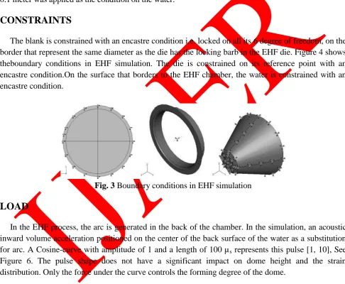
CONSTRAINTS

The blank is constrained with an encastre condition i.e. locked on all its 6 degree of freedom, on the border that represent the same diameter as the die has the locking barb in the EHF die. Figure 4 shows theboundary conditions in EHF simulation. The die is constrained on its reference point with an encastre condition.On the surface that borders to the EHF chamber, the water is constrained with an encastre condition.

Fig. 3 Boundary conditions in EHF simulation

LOAD

In the EHF process, the arc is generated in the back of the chamber. In the simulation, an acoustic inward volume acceleration positioned on the center of the back surface of the water as a substitution for arc. A Cosine-curve with amplitude of 1 and a length of 100 µs represents this pulse [1, 10], See

52 Fig. 4 Acoustic Acceleration pulse model [1]

The relation between the input energy in the experiment and the input volume acceleration in the simulation should be obtained correctly. But the relation is complex and creating this relation is a tough job. For this purpose, for grade IF210, a reference magnitude of the pulse is set, so that the height of the formed blank in simulation and the height of the dome in the EHF experiment reach the same amount. For determination of the volume acceleration for other grades, the reference magnitude is recounted regarding to the respective input energy in the experiment. According to the Equation 11, the magnitude of grades (the acceleration) correspond with the square of the change relative to the reference magnitude. In Equation 11,E is the energy, q is the changing fraction of the input energy, and p is the changing fraction of the acceleration.

ELEMENT TYPE AND MESH FOR BLANK

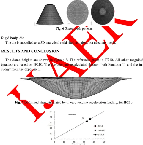
A 3D deformable shell chose for the blank. Element type S4R; a 4-node doubly curved thin or thick shell, reduced integration, hourglass control, finite membrane strains.A quadratic mesh with a global seeding of 3 millimeters was applied. On the edge of the blank, much more refined seeding of 0.5 millimeters in the radius direction was considered. This mesh size was mandatory to determine the rounded edge on the die, and a smooth strain distribution.

53

ELEMENT TYPE AND MESH FOR WATER

A 3D deformable solid was considered for the water. Element type AC3D8R was applied for the water: This element is an 8-node linear acoustic brick, reduced integration, hourglass control. The element is a hexagonal acoustic type with a seeding of 50 elements on one base diameter (4 millimeters) and element height of 13 millimeters.

Fig. 6 Sheet mesh pattern

Rigid body, die

The die is modelled as a 3D analytical rigid shell and does not need any mesh.

RESULTS AND CONCLUSION

The dome heights are shown in figures 8. The reference grade is IF210. All other magnitudes (grades) are based on IF210. These grades are recalculated through both Equation 11 and the input energy from the experiment.

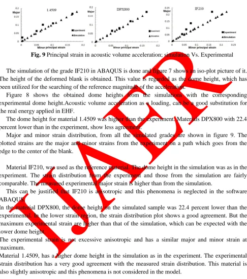
Fig. 7 Deformed sheet simulated by inward volume acceleration loading, for IF210

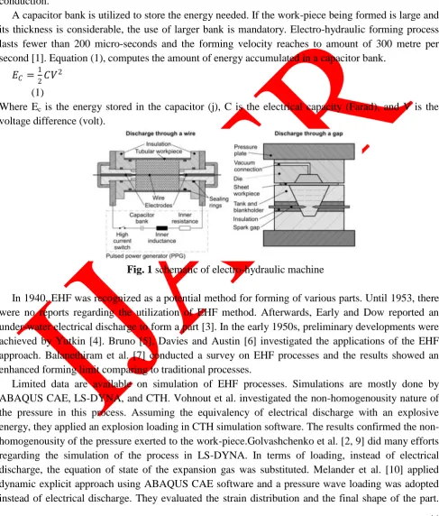
54 Fig. 9 Principal strain in acoustic volume acceleration; simulation Vs. Experimental

The simulation of the grade IF210 in ABAQUS is done and figure 7 shows an iso-plot picture of it. The height of the deformed blank is obtained. This value is regarded as the dome height, which has been utilized for the searching of the reference magnitude of the acceleration.

Figure 8 shows the obtained dome heights from the simulations with the corresponding experimental dome height.Acoustic volume acceleration as a loading, can be a good substitution for the real energy applied in EHF.

The dome height for material 1.4509 was higher than the experiment. Materials DPX800 with 22.4 percent lower than in the experiment, show less agreement.

Major and minor strain distribution, from all the simulated grades are shown in figure 9. The plotted strains are the major and minor strains from the experiment on a path which goes from the edge to the center of the blank.

Material IF210, was used as the reference material. The dome height in the simulation was as in the experiment. The strain distribution from the experiment and those from the simulation are fairly comparable. The measured experimental major strain is higher than from the simulation.

This can be justified that IF210 is anisotropic and this phenomena is neglected in the software ABAQUS.

In the material DPX800, the dome height on the simulated sample was 22.4 percent lower than the experimental. In the lower strain region, the strain distribution plot shows a good agreement. But the maximum experimental strain are higher than that of the simulation, which can be expected with the lower dome height.

The experimental strain is not excessive anisotropic and has a similar major and minor strain at maximum.

Material 1.4509, has a higher dome height in the simulation as in the experiment. The experimental strain distribution has a very good agreement with the measured strain distribution. This material is also slightly anisotropic and this phenomena is not considered in the model.

REFERENCES

[1] D.Bjorkstrom, FEM Simulation of Electrohydraulic Forming. In: KTH (Kungliga Tekniska

55

[2] S.Golovashchenko, J.Gillard, V. Mamutov, Formability of Dual Phase Steels in Electrohydraulic

Forming. In: Journal of Materials Processing Technology, pp. 1191–1212, 2013

[3] C. Early, W. G. Dow. Experimental Studies and Applications of Explosive Pressure Produced by

Sparks in Confined Channels, Conference paper presented during the A.I.E.E. Winter Meeting January 19th to 23rd . New York, pp. 110-180, 1953

[4] L.A. Yutkin, Electrohydraulic Effect, Mashgiz (in Russian). Moscow, Russia, 1955

[5] E.J. Bruno, High-Velocity Forming Of Metals, Dearborn, MI, USA, American Society of Tool and Manufacturing Engineers, 1968

[6] R. Davies, E.R. Austin, Development in High Speed Metal Forming, New York, USA, Industrial Press Inc, 1970

[7] V.S. Balanethiram, G.S. Daehn, Hyperplasticity: Increased Forming Limits At High Workpiece

Velocity. Ph.D Dissertation. Ohio State University, vol. 30, pp. 515-520, 1994

[8] V. J. Vohnout, G.S. Daehn, G. Fenton, Pressure Heterogeneity in Small Displacement

Electrohydraulic Forming Processes. In: Proceedings of 4th International Conference on High Speed Forming, pp. 65-74, 2010

[9] S. Golovashchenko, R. Ibrahim, V. Mamutov, J. Bonnen, L. Smith, Analysis of Contact Stresses

in High Speed Sheet Metal Forming Processes. In: 5th International Conference on High Speed Forming, pp. 1170-1175; 2012

[10] A. Melander, A. Delic, A. Björkblad, P. Juntunen, L. Samek, L. Vadillo, Modelling of Electro

hydraulic Free and Die Forming of Sheet Steels, Int J Mater Form 6, pp. 223–231, 2013

[11] M. Farzin, H. Montazerolghaem, Manufacture of Thin Miniature Parts Using Electrohydraulic

Forming and Viscous Pressure Forming Methods, Accepted by Journal of Archives of Metallurgy and Materials, to be published in volume 54, pp. 501-513, 2009

[12] K. Lei, N. Li, H. Huang, J. Huang, J. Qu. The Characteristics of Underwater Plasma Discharge

Channel and Its Discharge Circuit. College of Marine Engineering Northwestern Poly-technical University, In: China, pp. 619-626, 20011

[13] S. Buogo, J. Plocek, K. Vokurka, Efficiency of Conversion in Underwater Spark Discharges and

Associated Bubble Oscillations: Experimental Results. In: JASA, pp. 9-16, 23 November 2006

[14] M. Oyane, S. Masaki, Fundamental Study on Electrohydraulic Forming 2. In: The Japan Society of Mechanical Engineers, V.8, pp. 251-258, No 30; 1965

[15] M.K. Knyazyev, Ya. S. Zhovnovatuk, Measurements of Pressure Fields with Multi-Point

Membrane Gauges at Electrohydraulic Forming. In: Proceedings of 4th International Conference on High Speed Forming, pp. 75-82, 2010

[16] A. Sayapin, A. Grinenko, S. Efimov, Y. E. Krasik, Comparison of Different Methods of

56

[17] V. Mamutov, S. Golovashchenko, A. Mamutov, Simulation of High-Voltage Discharge Channel

in Water at Electro-Hydraulic Forming Using LS-DYNA. In: 13th International LS-DYNA Users Conference, Metal Forming, pp. 1-9, 2012

[18] I. Gilchrist, B. Crossland, The Forming of Sheet Metal using and Underwater Electrical

Discharge. In: Proceedings of the Conference on Electrical Methods of Machining and Forming, pp. 92-113, 1967

[19] L. Coman. The Influence of Some Factors on Maximum Depth in Electrohydraulic Forming. In:

U.E.M. Resita, Romania, Journal No 2, pp. 93-98, 2010

[20] A. Rohatgi, E.V. Stephens, A. Soulami, R.W. Davies, M.T. Smith, Experimental Characterization

of Sheet Metal Deformation During Electrohydraulic Forming. Journal of Materials Processing Technology 211, pp. 1824–1833, 2011

[21] S. Golovashchenko, J. Gillard, J.F. Mamutov, S. Bonnen, V. Dawson, Electro-hydraulic Sheet

Metal Forming of Aluminum Panels. In: TMS (The Minerals, Metals & Materials Society), pp. 449-454, 2012

[22] M. Saghafi, R. Hooshmand, High Voltage Engineering and Insulating, Second Edition, Shahid Chamran University Press, Ahvaz, Iran, pp 50-190, 2013 (In Persian)

[23] L. Coman, C. Hamat. The Influence of Distance between Electrodes at Electrohydraulic Forming.

In: U.E.M. Resita, Romania, Journal No 3, pp. 1453-7397, 2011

[24] M. Woetzel, M.J. Löffler, E. Spahn, H. Ritter, Preliminary Examination of High-Velocity

Metal-shaping with Electrical Wire Explosion, pp. 1-6, 2010

[25] M. Oyane, S. Masaki, Fundamental Study on Electrohydraulic Forming. In: The Japan Society of Mechanical Engineers, V. 8, pp. 259-263, No. 30, 1965

[26] T. Hasebe, Y. Takenaga, H. Kakimoto, Y. Imaida, High Strain Rate Forming Using an

Underwater Shock Wave Focusing Technique. In: Journal of Materials Processing Technology