MathCode: A System for C++ or Fortran Code Generation from Mathematica »

(1)

MathCode: A System

for C++ or Fortran

Code Generation from

Mathematica

Peter Fritzson

Vadim Engelson

Krishnamurthy Sheshadri

MathCode is a package that translates a subset of Mathematica into a

com-piled language like Fortran or C++. The chief goal of the design of

Math-Code is to add extra performance and portability to the symbolic

prototyp-ing capabilities offered by Mathematica. This article discusses several important features of MathCode, such as adding type declarations, exam-ples of functions that can be translated, ways to extend the compilable subset, and generating a stand-alone executable, and presents a few applica-tion examples.

‡

Introduction

MathCode is a Mathematica add-on that translates a Mathematica program into C++ or Fortran 90. The subset of Mathematica that MathCode is able to translate involves purely numerical operations, and no symbolic operations. In the following sections we provide a variety of examples that show precisely what we

mean. The code that is generated can be called and run from within Mathematica,

as if you were running a Mathematica function.

There are two important purposes that are served by MathCode. Firstly, the C++/

(2)

about 50 to 100) over interpreted (compiled) Mathematica code, resulting in considerable performance gains, while still requiring hardly any knowledge of C++/Fortran 90 on the part of the user. Secondly, the generated code can also be executed as a stand-alone program outside Mathematica, offering a portability otherwise not possible. You should note, however, that these advantages come at some loss of generality since integer and floating point overflow are not trapped and switched to arbitrary precision as in standard Mathematica code. Here the

avoid such problems. The measurements in this article were made using

Mathe-matica 6.

There are situations in which having a system such as MathCode can be

particu-larly helpful and effective, like when a certain calculation involves a symbolic phase followed by a numerical one. In such a hybrid situation, Mathematica can be employed for the symbolic part to give a set of expressions involving only

numerical operations that can be made part of a Mathematica function, which can

then be translated into C++/Fortran 90 using MathCode.

In this article, we describe some of the more important features of MathCode. For a more detailed discussion the reader is referred to [1]. For brevity, we simply say

C++ when we actually mean C++ or Fortran 90: MathCode can generate code in

both C++ and Fortran, although we illustrate C++ code generation in this article.

In Section 2, we show how to quickly get started with MathCode using a simple

example of a function to add integers.

Section 3 presents many useful features of MathCode. In Section 3.1, we discuss the way the system works, the various auxiliary files generated and what to make of them, and how to build C++ code and install the executable. We then compare the execution times of the interpreted Mathematica code and the compiled C++ code. This section also illustrates how MathCode works with packages.

Section 3.2 briefly makes a few points about types and type declarations in

Math-Code. There are two ways to declare argument types and return types of a

func-tion menfunc-tioned in this secfunc-tion.

In Section 3.3, we show how to generate a stand-alone C++ executable. This executable can be run outside of Mathematica. We illustrate how to design a suit-able main program that the executsuit-able runs.

It should be emphasized that MathCode can generate C++ for only that subset of Mathematica functions referred to as the compilable subset. Section 3.4 gives a sample of this subset, while Section 3.5 presents three ways to extend it with the already-available features of MathCode: Sections 3.5.1 through 3.5.3 discuss, respectively, symbolic expansion of function bodies, callbacks to Mathematica, and handling external functions. Each of these extensions has its own strengths and limitations.

Section 3.6 discusses common subexpression elimination, a feature that is aimed at enhancing the efficiency of generated code.

Section 3.7 presents some shortcuts available in MathCode to extract and make assignments to elements of matrices and submatrices, while Section 3.8 is about array declarations.

In Section 4, we present several examples of effectively using MathCode. Section 4.1 provides a summary of the examples.

Section 4.2 discusses an essentially simple example, that of computing the func-tion sinHx+yL over a grid in the x-y plane, but done in a somewhat roundabout manner so as to illustrate various features of MathCode.

Section 4.3 discusses an implementation of the Gaussian elimination algorithm [2] to solve matrix systems of the type A.X=B, where A is a square matrix of size n and X (the solution vector) and B are vectors of size n. In this section, we make a detailed performance study by computing the solution of a matrix

make comparisons with LinearSolve.

MathCode: A System for C++ or Fortran Code Generation from Mathematica 741

(3)

of size n and X (the solution vector) and B are vectors of size n. In this section,

system by turning on a few compilation options available in MathCode, and also

make comparisons with LinearSolve.

In Section 4.4, we show how to call external libraries and object files from a C++

program that is automatically generated by MathCode. We take the example of a

well-known matrix library called SuperLU [3], and demonstrate how to solve, using one of its object modules, a sparse matrix system arising from a partial differ-ential equation.

The MathCode User Guide that is available online discusses more advanced aspects, like a detailed account of types and declarations, the numerous options available in MathCode with the aid of which the user can control code generation and compilation, and other features. We refer interested readers to [1].

In Section 5, we summarize the salient aspects of MathCode and discuss the kinds of applications for which MathCode is particularly useful. We conclude the article with a brief summary of various points made. The first version of MathCode, released in 1998, was partly developed from the code generator in the Object-Math environment [4, 5]. The current version is almost completely rewritten and very much improved.

‡

2. Getting Started with

MathCode

· 2.1. An Example Function

In this section we take the reader on a quick tour of MathCode using the simple

example of a function to add integers.

The following command loads MathCode.

In[1]:= Needs@"MathCode`"D

MathCode C++1.4.0 for mingw32 loaded from C:\MathCode

MathCode works by generating a set of files in the current directory (see Section 3.1). We can set the directory in the standard way as follows; here,

$MCRoot is the MathCode root directory. The user can, however, use any other directory to store the files.

In[2]:= SetDirectory@$MCRoot<>"êDemosêSimplestExample"D;

Let us now define a Mathematica function sumint to add the first n natural numbers.

In[3]:= sumint@n_D:=

Module@8res=0, i<, For@i=1, i§n, i++, res=res+iD; resD

(4)

· 2.2. Declaration of Types

We must now declare the data types of the parameter n and the local variables res

and i; we must also specify the return type of the function. We do this using the function Declare that MathCode provides.

In[4]:= Declare@sumint@Integer n_DØInteger,8Integer, Integer<D;

Note that Integer n_does not mean Integer*n_; the function Declare creates an environment in which this is interpreted as a type declaration, that is, an integer variable n is being declared in the example. The type Integer is trans-lated to a native C int type, and the type Real to a native C double type.

· 2.3. C++ Code

To generate and compile the C++ code, we execute the following command.

In[5]:= BuildCode@"Global`"D;

Successful compilation to C++: 1 functionHsL

Since we have not specified the context of sumint, its default context is Global. We could, therefore, have simply executed the following command instead.

In[6]:= BuildCode@D;

With the following command, we seamlessly integrate an external program with

Mathematica.

In[7]:= InstallCode@D;

Global is installed.

We can now run the external program in the same way that we would execute a

Mathematica command. In[8]:= sumint@1000D

Out[8]= 500 500

If we want to run the Mathematica code (and not the generated C++ code) for

sumint, we must first uninstall the C++ executable.

In[9]:= UninstallCode@D;

Now the Mathematica code for sumint will run. In[10]:= sumint@1000D

Out[10]= 500 500

(5)

‡

3. A Tour of

MathCode

· 3.1. How the MathCode System Works

MathCode works by generating a set of files in the home directory. In the example of sumint, the default context is Global and the files generated by Math-Code are: Global.cc (the C++ source file), Global.h and Global.mh (the header files), Globaltm.c, Global.tm and Globalif.cc (the MathLink”-related files that enable transparently calling C++ versions of the function sumint from Mathe-matica), and Globalmain.cc, which contains the function main( ) needed when building a stand-alone executable.

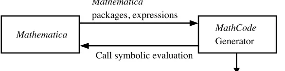
We can also create a package (let us call it foo) that defines its own context foo

instead of the default context Global. See Figure 1 for a block diagram of the way the overall system works. The MathCode code generator translates the Mathe-matica package to a corresponding C++ source file foo.cc. Additional files are automatically generated: the header file foo.h, the MathCode header file foo.mh, the MathLink-related files footm.c, foo.tm, foo.icc, and fooif.cc, which enable calling the C++ versions from Mathematica, and foomain.cc, which contains the function main that is needed when building a stand-alone executable for foo (see Section 3.3). The generated file foo.cc created from the package foo, the header file foo.h, and additional files are compiled and linked into two executables. In the case of MathCode F90, Fortran 90 is generated and a file foo.f90 is created. No header file is generated in that case since Fortran 90 provides directives for the use of module. External numerical libraries may be included in the linking process by specifying their inclusion (Sections 3.5.3 and 4.5). The executable produced, foo.exe, can be used for stand-alone execution, whereas fooml.exe is

used when calling on the compiled C++ functions from Mathematica via

MathLink.

Mathematica MathCode

Generator Call symbolic evaluation

Mathematica

packages, expressions

foo.cc, foo.h, foomain.cc, footm.c, foo.tm, fooif.cc, foo.mh

Figure 1. Generating C++ code with MathCode for a package called foo.

Let us see how to work with a package again using the same sumint example.

In[1]:= Needs@"MathCode`"D;

(6)

If we are compiling the package foo using MathCode, we also need to mention

MathCodeContexts within the path of the package.

In[3]:= BeginPackage@"foo`",8MathCodeContexts<D;

We define the function sumint

In[4]:= sumint@n_D:=

Module@8res=0, i<, For@i=1, i§n, i++, res=res+iD; resD;

and close the context foo.

In[5]:= EndPackage@D;

We next declare the types, and then build and install as before.

In[6]:= Declare@sumint@Integer x_DØInteger,8Integer, Integer<D;

In[7]:= BuildCode@"foo`"D;

Again, since the package foo has been defined, it is the default context, and so we could simply have executed the following command.

In[8]:= BuildCode@D;

To run the executable from the notebook, we must install it.

foo is installed.

Now the following command runs the C++ executable fooml.exe. The call to

sumint via MathLink is executed 1000 times. The timing measurement includes

MathLink overhead, which typically for small functions is much more than the execution time for the compiled function. This can be avoided if the loop is executed within the external function itself, as in the example in Section 4.2.5.

In[10]:= Timing@Do@res=sumint@1000D,81000<D; resD

Out[10]= 81.392, 500 500<

(7)

Here is the C++ code that was generated.

In[11]:= FilePrint@"foo.cc"D

#include "foo.h"

#include "foo.icc"

#include <math.h> void foo_TfooInit () {

; }

int foo_Tsumint ( const int &n) {

int res = 0; int i; i = 1;

while (i <= n) {

res = res+i; i = i+1; }

return res; }

Note that the function sumint appears as foo_Tsumint in the generated code. This is because the full name of the function is in fact foo`sumint, and Math-Code replaces the backquote "`" by "_T" in the C++ code.

To run the Mathematica function (and not its C++ equivalent) sumint, we must use the following command to uninstall the C++ code.

Now it is the Mathematica code that runs when you execute sumint. In[13]:= Timing@Do@res=sumint@1000D,81000<D; resD

Out[13]= 822.161, 500 500<

You can see that the C++ executable together with the MathLink overhead runs

about 15 times faster than the Mathematica code. The factor by which the perfor-mance is enhanced is problem dependent, however. The perforperfor-mance of the

Mathematica code could also have been improved by using the built-in Compile

function. In Section 4 we will see many more examples, some quite involved, where we get a range of performance enhancements, also including usage of the

Compile function.

We clean up the current directory by removing the files automatically generated by MathCode.

(8)

· 3.2. Types and Declarations

To be able to generate efficient code, the types of function arguments and return values must be specified, as we have seen in the preceding examples. The basic types used by MathCode are

8Real, Integer, Null<

Arrays (vectors and matrices) of these types can also be declared.

8Real@5D, Real@3, 4D, Real@_D, Integer@m, nD, Integer@2, 3, n_D<

Type declarations can be given in two different ways:

Ë Directly in the function definition

f@Real x_DØReal :=x2

Ë In a separate command

g@x_D:=Sin@xD

Declare@g@Real x_DØRealD

The latter construction can be useful if you want to separate already existing

Mathematica code with the type information needed to be able to generate C++ code using MathCode.

· 3.3. Generating a Stand-Alone Program

So far we have only seen examples in which the installed C++ code can be run within Mathematica. However, we can also produce a stand-alone executable. This offers a degree of portability that can be useful in practice.

To illustrate, we take the same example function sumint that we discussed in the previous sections. The sequence of commands is very much as in the previous section, except for the option StandAloneExecutableØTrue for the MathCode

function MakeBinary, and an appropriate option MainFileAndFunction for the

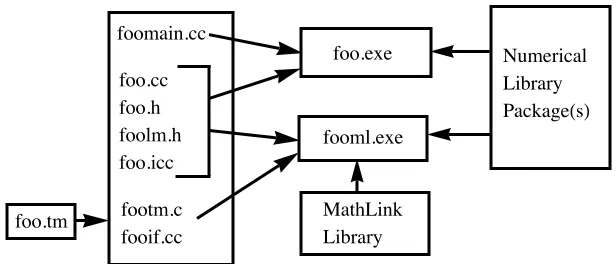
function SetCompilationOptions immediately after BeginPackage. Figure 2

illustrates the process of building the two kinds of executable, namely fooml.exe and foo.exe (on some systems foomain.exe) from a package called foo.

The option MainFileAndFunction is used to specify the main file. The func-tions defined in Mathematica must have the prefix Global_T (packagename_T in general) to be recognized in the main file.

(9)

Numerical Library PackageHsL

MathLink Library fooml.exe

foo.exe foomain.cc

foo.cc foo.h foolm.h foo.icc

footm.c fooif.cc foo.tm

Figure 2. Building two executables from the package foo, possibly including numerical libraries.

In[18]:= SetCompilationOptions@

MainFileAndFunctionØ"Òinclude<stdio.h>\n int mainHL

8int n;printfH\"give an integer:\"L;scanfH\"%d\",&nL;printfH\"the sum is%d.\n\",foo_TsumintHnLL;return 0;<

"D;

In[19]:= sumint@n_D:=

Module@8res=0, i<, For@i=1, i§n, i++, res=res+iD; resD;

In[20]:= EndPackage@D;

In[21]:= Declare@sumint@Integer x_DØInteger,8Integer, Integer<D;

Now we are ready to generate and compile the C++ code for the package foo.

We can do this in two ways: we can either employ the MathCode function BuildÖ

Code, as in the previous examples, or first execute CompilePackage (which

gener-ates the C++ source and header files) and then the function MakeBinary (which

creates the executable).

In[22]:= CompilePackage@"foo`"D;

In[23]:= MakeBinary@"foo`", StandAloneExecutableØTrueD;

The last command generates the stand-alone executable foo.exe that can be

executed from a command line, or, alternatively, by using the Mathematica

func-tion Run.

In[24]:= Run@"foo.exe"D

Out[24]= 0

If you desire, you can, in addition to the stand-alone executable foo.exe, also generate fooml.exe that can be run from within Mathematica, just like before.

(10)

foo is installed.

Now the following command runs the C++ program foo.cc.

In[27]:= sumint@1000D

Out[27]= 500 500

3.3.1. Generating a DLL

Here we briefly mention the possibility of generating a DLL, without giving a full example. To generate a DLL from a package, you have to write a file containing one simple wrapper function in order to make a generated function visible outside the DLL. You write a wrapper function for each generated func-tion. The flags used are as follows:

CompilePackage@NeedsExternalObjectModuleØ"ext"D;

MakeBinary@StandAloneExecutableØTrue, LinkerOptionsØ"êDLL"D

Here "ext.cpp" is a C++ file with wrapper functions, and "/DLL" is a flag for the Visual C++ linker. For other C++ compilers this procedure is not automatic and requires several operating system commands, but the wrapper functions are not needed.

· 3.4. The Compilable Subset

MathCode generates C++ code for a subset of Mathematica functions, called the

compilable subset. The following items give a sample of the compilable subset. For a complete list of Mathematica functions in the compilable subset, see [1].

Ë Statically typed functions, where the types of function arguments and return values are given by the types discussed in Section 3.2

Ë Scoping constructs: BeginPackage[ ], EndPackage[ ], Module[ ],

Block[ ], With[ ]

Ë Procedural constructs: For[ ], While[ ], If[ ], Which[ ], Do[ ]

Ë Lists and tables: List[ ], Table[ ], Array[ ], Range[ ], IdentityÖ

Matrix[ ]

Ë Size functions: Dimensions[ ], Length[ ]

Ë Arithmetic and logical expressions, for example: +, -, *, /, ==, !=, >, !,

&&, ||, and so forth

Ë Elementary functions and some others, for example: Sin[ ], Exp[ ],

ArcSin[ ], Sqrt[ ], Round[ ], Max[ ], Cross[ ], Transpose[ ], Dot[ ]

Ë Constants: True, False, E, Pi

Ë Assignments: :=, =

(11)

Ë Functional commands: Map[ ], Apply[ ]

Ë Some special commands: Sum[ ], Product[ ]

Functions not in the compilable subset can be used in external code by callbacks to Mathematica (see Section 3.5.2 for an example).

Examples of functions that are not a part of the compilable subset include:

Integrate[ ], Solve[ ], FindRoot[ ], LinearSolve[ ], Expand[ ], Factor[ ].

These functions can be used if Mathematica can evaluate them at compile time to

expressions that belong to the compilable subset. In general, Mathematica func-tions that perform symbolic operafunc-tions are not in the compilable subset. Also, many functions in the subset are implemented with limitations, that is, more diffi-cult cases are not always supported. However, MathCode currently provides several ways to extend the compilable subset, as we discuss in the next section.

· 3.5 Ways to Extend the Compilable Subset

3.5.1. Symbolic Expansion of Function Bodies

Functions not entirely written using Mathematica code in the compilable subset,

but whose definitions can be evaluated symbolically to expressions that belong to the compilable subset, can be handled by MathCode.

In[3]:= f@Real a_, Real b_DØReal :=Integrate@x Sin@xD,8x, a, b<D

In[4]:= f@1., 2.D

Out[4]= 1.44042

In[5]:= ? f

Global`f

f@a_, b_D:=_Ÿ_abx Sin@xD „x

Generate C++ code and compile it to an executable file.

In[6]:= BuildCode@EvaluateFunctionsØ8f<D

The option EvaluateFunctions tells MathCode to let Mathematica expand the function body as much as possible. Everything works fine because the result belongs to the compilable subset.

In[7]:= Integrate@x Sin@xD,8x, a, b<D

(12)

The generated executable is connected to Mathematica: In[8]:= InstallCode@D;

In[9]:= f@1., 2.D

Out[9]= 1.44042

3.5.2. Callbacks to Mathematica

Consider the following function whose definition includes the Zeta function, which does not belong to the compilable subset.

In[2]:= SetDirectory@$MCRoot<>"êDemosêSimplestExample"D

Out[2]= C:\MathCode\Demos\SimplestExample

In[3]:= f@x_D:=

Sin@xDCos@xD

1+Tan@xD2 ‰

-x2

Zeta@xD

Let us plot the function:

In[4]:= Plot@f@xD,8x, 2, 4<, PlotRangeØAllD

Out[4]=

2.5 3.0 3.5 4.0

-0.0020

-0.0015

-0.0010

-0.0005

We now make the declarations:

In[5]:= Declare@f@Real x_DØRealD

In[6]:= Declare@Zeta@Real x_DØRealD

These declare statements do not change the way Mathematica computes the function.

In[7]:= :[email protected], fB

5

2F>

Out[7]= :-0.000796932,

CosA5

2ESinA 5 2EZetaA

5 2E

‰25ê4_J₁₊_Tan_A5 2E

2

N >

Let us now generate C++ code and compile it to an executable file. The option

CallBackFunctions tells MathCode which functions have to be evaluated by

Mathematica. As a result, although the function Zeta is not in the compilable subset, an executable is still generated and communicates with the kernel to

(13)

Let us now generate C++ code and compile it to an executable file. The option

CallBackFunctions tells MathCode which functions have to be evaluated by

Mathematica. As a result, although the function Zeta is not in the compilable subset, an executable is still generated and communicates with the kernel to eval-uate Zeta.

In[8]:= BuildCode@CallBackFunctionsØ8Zeta<D

The generated executable is connected to Mathematica: In[9]:= InstallCode@D;

Now it is the external code that is used to compute the function:

In[10]:= :[email protected], fB

5

2F>

Out[10]= :-0.000796932, fB

5 2F>

In this case the external code calls Mathematica when the Zeta function has to be evaluated. After the evaluation the computation proceeds in the external code. Note that it is the installed code for the function f that is executed above, and not the original Mathematica function. In the installed code, the argument of f

must be real, according to our declaration. As a result, f[5/2], in which we pass a rational number as an argument, is left unevaluated.

We again plot the function, but this time using the external code to evaluate it:

In[11]:= Plot@f@xD,8x, 2, 4<, PlotRangeØAllD

Out[11]=

2.5 3.0 3.5 4.0

-0.0020

-0.0015

-0.0010

-0.0005

3.5.3. External Functions

We can have references to external objects in C++ code generated by MathCode.

Let us consider three very simple external functions that compute x2_,_ex_{, and}

(14)

In[2]:= SetDirectory@$MCRoot<>"êDemosêOverview"D;

In[3]:= FilePrint@"external1.cc"D

#include <math.h>

extern double extsqr(const double &x) { return x*x;

}

extern double extexp(const double &x) { return exp(x);

}

extern double extoscillation(const double &x) {

return sin(x); }

Observe here that each function definition, which is in C language syntax, is followed by a “wrapper” that enables MathCode to recognize the object as external. We can then create an object file corresponding to these functions and link the object as follows.

In[4]:= extsqr@Real x_DØReal :=ExternalFunction@D;

extexp@Real x_DØReal :=ExternalFunction@D;

extoscillation@Real x_DØReal :=ExternalFunction@D;

We define a function to create a list of numbers using the external functions.

In[7]:= Makeplot@Integer n_DØReal@nD:=Module@8Integer i, Real@_Darr<,

arr=Table@extsqr@[email protected] extexp@[email protected],8i, n<D; arrD

We now compile the package. Since this is a very small example, we do not bother to create a special package for the code.

In[8]:= CompilePackage@D

Let us now create the MathLink binary; to do this when there are external

func-tions, we must specify the option NeedsExternalObjectModule as follows.

In[9]:= MakeBinary@NeedsExternalObjectModuleØ8"external1"<D

Here, as we noted above, external1 and external2 represent the external object modules external1.o and external2.o. Install the MathCode-compiled code so it is called using MathLink.

(15)

When we make the following plot, it is the external code for extsqr, extexp, and extoscillation that is used.

In[11]:= ListPlot@Makeplot@100D, JoinedØTrueD

Out[11]=

20 40 60 80 100

0.2 0.4 0.6 0.8

· 3.6. Common Subexpression Elimination

Consider the following function whose definition contains a number of common

subexpressions (e.g., 1+x2_and ₁₊_x2_).

In[2]:= g@Real x_DØReal :=

x Cos@xDCosB 1+x2 _F

H1+x2_L3ê2_I₁₊_Cos_@_x_D2_M

-2 x Cos@xDSinB 1+x2 _F

H1+x2_L2_I₁₊_Cos_@_x_D2_M +

2 Cos@xD2Sin@xDSinB 1+x2 _F

H1+x2_{L I}₁₊_Cos_@_x_D2_M2

-Sin@xDSinB 1+x2 _F

H1+x2_{L I}₁₊_Cos_@_x_D2_M

There are very efficient algorithms to evaluate functions containing common subexpressions. The basic idea is to evaluate common subexpressions only once and put the results in temporary variables.

Now we generate C++ code using MathCode and run it.

In[3]:= BuildCode@D

(16)

In[5]:= Timing@Do@[email protected],8100<DD

Out[5]= 80.15, Null<

MathCode does common subexpression elimination (CSE) when the option

EvaluateFunctions is given to CompileCode[ ] or BuildCode[ ]. This basic strategy could be further improved for special cases in future versions of Math-Code. Moreover, since mathematical expressions are intrinsically free of side effects and do not have a specific evaluation order, the CSE optimization may change the order of computing subexpressions if this improves performance. Changing the order can sometimes have a small influence on the result when floating-point arithmetic is used.

In[7]:= CleanMathCodeFiles@ConfirmØFalse, CleanAllButØ8<D;

In[8]:= BuildCode@EvaluateFunctionsØ8g<D

In[10]:= Timing@Do@[email protected],8100<DD

Out[10]= 80.21, Null<

We take a look at the generated C++ file.

In[11]:= FilePrint@"Global.cc"D

#include "Global.h"

#include "Global.icc"

#include <math.h>

void Global_TGlobalInit () {

; }

double Global_Tg ( const double &x) { double mc_T1; double mc_T2; double mc_T3; double mc_T4; double mc_T5; double mc_T6; double mc_T7; double mc_T8; double mc_T9; double mc_T10; double mc_T11; double mc_T12; double mc_T13; double mc_T14; double mc_T15; double mc_T16; double mc_T17; double mc_T18; double mc_T19; double mc_T20; double mc_T21; double mc_T22; double mc_T23; double mc_T24; double mc_T25; mc_T1 = (x*x); mc_T2 = 1+mc_T1; mc_T3 = cos(x); mc_T4 = (mc_T3*mc_T3); mc_T5 = 1+mc_T4; mc_T6 = mc_T5*mc_T2; mc_T7 = 0.5; mc_T8 = pow(mc_T2, mc_T7); mc_T9 = sin(mc_T8); mc_T10 = sin(x); mc_T11 = mc_T10*mc_T9; mc_T12 = mc_T11/mc_T6; mc_T13 = -mc_T12; mc_T14 = pow(mc_T5, -2);

mc_T15 = 2*mc_T4*mc_T14*mc_T10*mc_T9; mc_T16 = mc_T15/mc_T2;

mc_T17 = pow(mc_T2, -2);

mc_T18 = -2*x*mc_T17*mc_T3*mc_T9; mc_T19 = mc_T18/mc_T5;

mc_T20 = cos(mc_T8); mc_T21 = -1.5; mc_T22 = pow(mc_T2, mc_T21); mc_T23 = x*mc_T22*mc_T3*mc_T20; mc_T24 = mc_T23/mc_T5;

mc_T25 = mc_T24+mc_T19+mc_T16+mc_T13; return mc_T25;

}

(17)

#include "Global.icc"

#include <math.h>

void Global_TGlobalInit () {

; }

double Global_Tg ( const double &x) { double mc_T1; double mc_T2; double mc_T3; double mc_T4; double mc_T5; double mc_T6; double mc_T7; double mc_T8; double mc_T9; double mc_T10; double mc_T11; double mc_T12; double mc_T13; double mc_T14; double mc_T15; double mc_T16; double mc_T17; double mc_T18; double mc_T19; double mc_T20; double mc_T21; double mc_T22; double mc_T23; double mc_T24; double mc_T25; mc_T1 = (x*x); mc_T2 = 1+mc_T1; mc_T3 = cos(x); mc_T4 = (mc_T3*mc_T3); mc_T5 = 1+mc_T4; mc_T6 = mc_T5*mc_T2; mc_T7 = 0.5; mc_T8 = pow(mc_T2, mc_T7); mc_T9 = sin(mc_T8); mc_T10 = sin(x); mc_T11 = mc_T10*mc_T9; mc_T12 = mc_T11/mc_T6; mc_T13 = -mc_T12; mc_T14 = pow(mc_T5, -2);

mc_T15 = 2*mc_T4*mc_T14*mc_T10*mc_T9; mc_T16 = mc_T15/mc_T2;

mc_T17 = pow(mc_T2, -2);

mc_T18 = -2*x*mc_T17*mc_T3*mc_T9; mc_T19 = mc_T18/mc_T5;

mc_T20 = cos(mc_T8); mc_T21 = -1.5; mc_T22 = pow(mc_T2, mc_T21); mc_T23 = x*mc_T22*mc_T3*mc_T20; mc_T24 = mc_T23/mc_T5;

mc_T25 = mc_T24+mc_T19+mc_T16+mc_T13; return mc_T25;

}

Note how the computation of the function has been divided into small subexpres-sions that are evaluated only once and then stored in temporary variables for future use. This gives very efficient code for large functions. The speed enhance-ment of roughly 150% brought about by CSE in this example is not appreciable because the example itself is rather small.

· 3.7. Extended Matrix Operations

When dealing with matrices, it is very convenient to have a short notation for part extraction. MathCode extends the functionality of Part[ ] or [[ ]] to achieve this.

(18)

Consider the following 4µ5 matrix:

In[12]:= A=Table@a@i, jD,8i, 4<,8j, 5<D; AêêMatrixForm Out[12]//MatrixForm=

a@1, 1D a@1, 2D a@1, 3D a@1, 4D a@1, 5D a@2, 1D a@2, 2D a@2, 3D a@2, 4D a@2, 5D a@3, 1D a@3, 2D a@3, 3D a@3, 4D a@3, 5D a@4, 1D a@4, 2D a@4, 3D a@4, 4D a@4, 5D

We can extract rows 2 to 4 as follows, with the shorthand available in MathCode. In[13]:= AP2»4T êê MatrixForm

Out[13]//MatrixForm=

a@2, 1D a@2, 2D a@2, 3D a@2, 4D a@2, 5D a@3, 1D a@3, 2D a@3, 3D a@3, 4D a@3, 5D a@4, 1D a@4, 2D a@4, 3D a@4, 4D a@4, 5D

We can extract the elements in all rows that belong to column 3 and higher:

In[14]:= AP_, 3»_T êêMatrixForm Out[14]//MatrixForm=

a@1, 3D a@1, 4D a@1, 5D a@2, 3D a@2, 4D a@2, 5D a@3, 3D a@3, 4D a@3, 5D a@4, 3D a@4, 4D a@4, 5D

We can assign values to a submatrix of A.

In[15]:= AP2»3, 2»3T = 881, 2<,83, 4<<;

In[16]:= A êê MatrixForm Out[16]//MatrixForm=

a@1, 1D a@1, 2D a@1, 3D a@1, 4D a@1, 5D a@2, 1D 1 2 a@2, 4D a@2, 5D a@3, 1D 3 4 a@3, 4D a@3, 5D a@4, 1D a@4, 2D a@4, 3D a@4, 4D a@4, 5D

All these operations belong to the compilable subset and can result in compact

code. Note: A[[2|4]]] denotes the same Mathematica computation as

Take[A,{2,4},All], and A[[_, 3|_]] is equivalent to Take[A,All,{3,-1}].

· 3.8. Array Declaration and Dimension

In this subsection, we give a few examples of array declarations. There are two main cases to consider.

Ë Arrays that are passed as function parameters or returned as function values, where the actual array size has been previously allocated

Ë Declaration of array variables, usually specifying both the type and the allocation of the declared array

(19)

There are five allowed ways to specify array dimension sizes in array types for function arguments and results.

Ë Integer constant dimension sizes, for example: Real[3,4]

Ë Symbolic-constant dimension sizes, for example: Real[three, four]

Ë Unknown dimension sizes with unnamed placeholders, for example:

Real[_, _]

Ë Unknown dimension sizes with named placeholders, for example:

Real[n_, m_]

Ë Unknown dimension sizes with variables as dimension sizes, for exam-ple: Real[n, m]

The dimension sizes can be constant, in which case the size information is part of the type. Alternatively, the sizes are unknown and thus fixed later at runtime when the array is allocated. Such unknown dimension sizes are specified through named (e.g., n_) or unnamed (_) placeholders.

All arrays that are passed as arguments to functions have already been allocated at runtime. Thus, their sizes are already determined. These sizes might, however, be different for different calls. Therefore it is not allowed to specify conflicting dimension sizes through integer variables (e.g., Real[n, m]) in array types of function parameters or results, as can be done for ordinary declared variables. Only constants and named, or unnamed, placeholders are allowed.

We now give examples of the five different ways of specifying array dimension information in variable declarations. The examples show a global variable declara-tion using Declare, but the same kinds of declarations can also be used for local declarations in functions.

The fifth case is where sizes are specified through integer variables. This is needed to handle declaration and allocation of arrays for which the sizes are not determined until runtime.

Ë Integer constant dimension sizes using the array arr:

Declare@Real@3, 4DarrD;

Ë Symbolic constant dimension sizes:

Declare@Real@three, fourDarrD;

Ë Unknown dimension sizes with unnamed placeholders:

Declare@Real@_,_DarrD;

Ë Unknown dimension sizes with named placeholders:

Declare@Real@k_, m_DarrD;

Ë Unknown dimension sizes that are specified and fixed to the values of integer variables, for example, n, m (e.g., function parameters, local or global variables that are visible from the declaration):

(20)

Integer variables, such as n and m, are assumed to be assigned once; that is, their values are not changed after the initial assignment, so that the declared sizes of allocated arrays are kept consistent with the values of those variables. This single-assignment property is not checked by the current version of the system, however. Thus, the user is responsible for maintaining such consistency.

‡

4. Application Examples

· 4.1. Summary of Examples

In the following we present a few complete application examples using MathCode.

The first example application is a small Mathematica program called SinSurface

(Section 4.2), which has been designed to illustrate two basic modes of the code generator: compiling without symbolic evaluation (the default mode, in which the function body is translated into C++ as it is), and compilation preceded by symbolic expansion, which is indicated by setting the option EvaluateFuncÖ

tionsØTrue (the function body is expanded using symbolic operations, simpli-fied, and then translated).

The second example, presented in Section 4.3, is an implementation of the Gaussian elimination procedure to solve a linear algebraic system of equations (see any standard text on numerical techniques for a discussion of the procedure, e.g., [2]). Here we compile generated C++ code with various options and do a detailed performance analysis.

In Section 4.4, we discuss the example of SuperLU, an external library [3] that performs efficient sparse matrix operations. We give an example of a program useful in solving partial differential equations that calls the SuperLU library and some of its object modules to solve a matrix equation of the type A.X=B, where

A is a very sparse square matrix.

· 4.2. The SinSurface Application Example

Here we describe the SinSurface program example. The actual computation is

performed by the functions calcPlot, sinFun2, and their helper functions. The

two functions calcPlot and sinFun2 in the SinSurface package will be

trans-lated into C++ and are declared together with a global array xyMatrix.

The array xyMatrix represents a 21µ21 grid on which the numerical function

sinFun2 will be computed. The function calcPlot accepts five arguments: four of these are coordinates describing a square in the x-y plane and one is a counter

(iter) to make the function repeat the computation as many times as necessary

in order to measure execution time. For each point on a 21µ21 grid, the numeric function sinFun2 is called to compute a value that is stored as an element in the matrix representing the grid.

4.2.1. Introduction

The SinSurface example application computes a function (here sinFun2) over a two-dimensional grid. The function values are stored in the matrix xyMatrix.

The execution of compiled C++ code for the function sinFun2 is over 500 times

faster than evaluating the same function interpretively within Mathematica.

(21)

The function sinFun2 computes essentially the same values as sinHx+yL, but in a more complicated way, using a rather large expression obtained through converting the arguments into polar coordinates (through ArcTan) and then using a series expansion of both Sin and Cos, up to 10 terms. The resulting large symbolic expression (more than a page) becomes the body of sinFun2, and is

then used as input to CompileEvaluateFunction to generate efficient C++

code. The symbolic expression and the call to CompileEvaluateFunction is

in-itiated by using the EvaluateFunctions option.

4.2.2. Initialization

We first set the directory in which MathCode will store the auxiliary files, the C++ code, and executable, and then load MathCode.

In[2]:= SetDirectory@$MCRoot<>"êtest"D;

The SinSurface package starts in the usual way with a BeginPackage declara-tion that references other packages. MathCodeContexts is needed in order to call the code generation related functions.

In[3]:= BeginPackage@"SinSurface`",8MathCodeContexts<D;

Clear@"SinSurface`*"D;

Next we define possibly exported symbols. Even though it is not necessary here, we enclose these names within Begin["SinSurface‘"] … End[ ] as a kind of context bracket, since this can be put into a cell, which can be conveniently re-evaluated by itself if new names are added to the list.

In[5]:= Begin@"SinSurface`"D

xyMatrix; calcPlot; sinFun1; sinFun2; arcTan; sin; cos; plot; cplus; plotfile; End@D

Out[5]= SinSurface`

Now we set compilation options as follows. This defines how the functions and variables in the package should be compiled to C++. By default, all typed vari-ables and functions are compiled. However, the compilation process can be controlled in a more detailed way by giving compilation options to CompileÖ

Package or via SetCompilationOptions. For example, in this package the func-tion sinFun2 should be symbolically evaluated before being translated to code, because it contains symbolic operations; the functions sin, cos, and arcTan

(22)

ables and functions are compiled. However, the compilation process can be controlled in a more detailed way by giving compilation options to CompileÖ

Package or via SetCompilationOptions. For example, in this package the func-tion sinFun2 should be symbolically evaluated before being translated to code,

sin cos arcTan

should not be compiled at all, because they are expanded within the body of sinFun2. The remaining typed function, calcPlot, will be compiled in the normal way.

In[6]:= SetCompilationOptions@EvaluateFunctionsØ8sinFun2<,

UnCompiledFunctionsØ8sin, cos, arcTan<, MainFileAndFunctionØ"int mainHL8return 0;<"D;

4.2.3. The Body of the SinSurface Package

We begin the implementation section of the SinSurface package, where func-tions are defined. This is usually private, to avoid accidental name shadowing due to identical local variables in several packages.

In[7]:= Begin@"SinSurface`Private`"D;

Declare public global variables and private package-global variables:

In[8]:= Declare@Real@21, 21DxyMatrixD;

Taylor-expanded sin and cos functions called by sinFun2 are now defined, just for the sake of the example, even though such a series gives lower relative accu-racy close to zero. A substitution of the symbol z for the actual parameter x is necessary to force the series expansion before replacing with the actual parameter.

In[9]:= sin@Real@x_DDØReal :=Normal@Series@Sin@zD,8z, 0, 10<DD ê. zØx;

cos@Real@x_DDØReal :=Normal@Series@Cos@zD,8z, 0, 10<DD ê. zØx;

Define arcTan, which converts a grid point to an angle, called by sinFun2:

In[11]:= arcTan@Real@x_D, Real@y_DDØReal :=

If@x<0,p, 0D+IfBxã0, 1

2 Sign@yDp, ArcTanB y

xFF;

sinFun2 is the function to be computed and plotted, called by calcPlot. It pro-vides a computationally heavy (series expansion) and complicated way of calcu-lating an approximation to sinHx+yL. This gives an example of a combination of symbolic and numeric operations as well as a rather standard mix of arith-metic operations. The expanded symbolic expression, which comprises the body of sinFun2, is about two pages long when printed.

Note that the types of local variables to sinFun2 need not be declared, since setting the EvaluateFunctions option will make the whole function body be symbolically expanded before translation.

Note also that a function should be without side effects in order to be symboli-cally expanded before final code generation. For example, there should be no assignments to global variables or input/output, since the relative order of these actions when executing the code often changes when the symbolic expression is created and later rearranged and optimized by the code generator.

(23)

In[12]:= sinFun2@Real x_, Real y_DØReal :=

BlockB8r, xx, yy<,

r= x2₊_y2 _;

xx=r cos@arcTan@x, yDD; yy=r sin@arcTan@x, yDD;

sin@xx+yyDF

The function calcPlot calculates data for a plot of sinFun2 over a 21µ21 grid, which is returned as a 21µ21 array.

In[13]:= calcPlot@Real xmin_, Real xmax_, Real ymin_,

Real ymax_, Integer iter_DØReal@21, 21D:=

ModuleB8Integer n=20, Real8x, y<, Integer8i, j, count<<,

ForBcount=1, count§iter, count=count+1,

ForBi=1, i§n+1, i=i+1,

ForBj=1, j§n+1, j=j+1,

x=xmin+Hxmax-xminL Hi-1L

n ; y=ymin+

Hymax-yminL Hj-1L

n ;

xyMatrixPi, jT=sinFun2@x, yDFFF;

xyMatrixF

In[14]:= End@D

EndPackage@D;

Out[14]= SinSurface`Private`

4.2.4. Execution

We first execute the application interpretively within Mathematica, and then use

Compile on the key function and execute the application again. Then we compile the application to C++, build an executable, and call the same functions from

Mathematica via MathLink.

Let us first do the Mathematica evaluation and plot.

In[16]:= meval=Timing@plot=calcPlot@-2., 2.,-2., 2., 20DDP1T ê20

(24)

In[17]:= ListPlot3D@plotD

Out[17]=

Next, we redefine sinFun2 to become a compiled version, using Mathematica’s standard Compile.

In[18]:= sinFun2=Compile@8x, y<, Evaluate@sinFun2@x, yDDD;

In[19]:= compeval=Timing@plot=calcPlot@-2., 2.,-2., 2., 100D;D

Out[19]= 87.109, Null<

In[20]:= compeval=compevalP1T ê100

Out[20]= 0.07109

In[21]:= sinFun2=.

4.2.5. Using the MathCode Code Generator

Compile the SinSurface package.

In[22]:= CompilePackage@"SinSurface"D

MathCodeConv`defConv::untypedlocalvars : Warning: Untyped local variableHsL:

8SinSurface`Private`r, SinSurface`Private`xx, SinSurface`Private`yy<in function with head sinFun2@SinSurface`Private`x_, SinSurface`Private`y_D. Real typeHsLassumed

The warnings concern local variables in sinFun2 that have no type information.

This is not important because those variables disappear upon symbolic expansion. The command MakeBinary compiles the generated code using a compiler (g++ in the present case). The object code is by default linked into the executable SinSurfaceml.exe for calling the compiled code via MathLink.

In[23]:= MakeBinary@D;

If any problems are encountered during code compilation, then warning and

error messages are shown. Otherwise no messages are shown. When MakeÖ

Binary is called without arguments, the call applies to the current package.

(25)

The command InstallCode installs and connects the external process

containing the compiled and linked SinSurface code.

In[24]:= InstallCode@"SinSurface"D

SinSurface is installed.

Out[24]= LinkObject@".\SinSurfaceml.exe", 14, 7D

Execute the generated C++ code for calcPlot.

In[25]:= AbsoluteTiming@[email protected], 2.0,-2.0, 2.0, 3000D;D

Out[25]= 83.6408347, Null<

Since the external computation was performed 3000 times, the time needed for one external computation is

In[26]:= externaleval=

%P1T 3000

Out[26]= 0.0012136116

Check that the result appears graphically the same.

In[27]:= ListPlot3D@plotD

Out[27]=

4.2.6. Performance Comparison

Let us now compare the running times for the three cases, the standard

Mathe-matica, compiled Mathematica, and the generated C++ code. In[28]:= 8mevalêexternaleval, compevalêexternaleval<

Out[28]= 8107.53, 58.5772<

The performance between the three forms of execution are compared in Table 1. The generated C++ code for this example is roughly 100 times faster than standard interpreted Mathematica code, and 50 times faster than code compiled by the internal Mathematica Compile command. This is on a Toshiba Satel-lite-2100, 400 Mhz AMD-K6, running Windows XP Pro SP2 and

(26)

-the inline directive is passed to -the C++ compiler for all functions to be compiled. If norange is specified, array element index range checking is turned off in the code generated by the C++ compiler, resulting in faster but less safe code.

We should emphasize that the comparisons in Table 1 are rather crude for several reasons. From a separate measurement, the loop part of calcPlot

excluding the call to sinFun2 comprises 25% of the total calcPlot time executed in interpreted Mathematica. The calcPlot function itself cannot be compiled using Compile, since it contains an assignment to a global matrix vari-able that cannot currently be handled by Compile. This might be regarded as

unfair to Compile. On the other hand, a MathLink overhead (divided by 500) in

returning the 21µ21 matrix is embedded in the figure for MathCode, which can

be regarded as unfair to MathCode. A better comparison for another small applica-tion example is available in Secapplica-tion 4.3.6.

In[29]:= TableForm@8

8"Execution Form", "Time consumed", "Relative"<,

8"StandardMathematica", meval, mevalêexternaleval<,

8"Compile@D", compeval, compevalêexternaleval<,

8"External C++viaMathLink", externaleval, 1<<D

Out[29]//TableForm=

Execution Form Time consumed Relative StandardMathematica 0.1305 107.53

Compile@D 0.07109 58.5772

External C++viaMathLink 0.0012136116 1

Table 1. Approximate performance comparison for the calcPlot example.

· 4.3. Gauss Application Example

4.3.1. Introduction

In this section, we present a textbook algorithm, Gaussian elimination (e.g., [2]), to solve a linear equation system. The given linear system, represented by a matrix equation of the type A.X=B, is subjected to a sequence of transforma-tions involving a pivot, resulting in the solution to the system, contained in the matrix X.

The following subsections illustrate the various aspects of the application.

4.3.2. Initialization In[1]:= Needs@"MathCode`"D

In[2]:= SetDirectory@$MCRoot<>$PathnameSeparator<>

"Demos"<>$PathnameSeparator<>"Gauss"D;

In[3]:= BeginPackage@"Gauss`",8MathCodeContexts<D;

(27)

Define exported symbols:

In[4]:= Begin@"Gauss`"D;

GaussSolveArraySlice; End@D;

4.3.3. Body of the Package

We now define the function GaussSolveArraySlice, based on the Gaussian

elimination algorithm.

In[7]:= Begin@"`Private`"D;

GaussSolveArraySlice@Real@n_, n_Dain_, Real@n_, m_Dbin_, Integer iterations_DØReal@n, mD:=

Module@8Real@nDdumc, Real@n, nDa, Real@n, mDb,

Integer@nD 8ipiv, indxr, indxc<, Integer8i, k, l, irow, icol<, Real8pivinv, amax, tmp<, Integer8beficol, afticol, count<<, For@count=1, count§iterations, count=count+1,Ha=ain;

b=bin;

For@k=1, k§n, k=k+1, ipiv@@kDD=0D; For@i=1, i§n, i=i+1,

H*find the matrix element with largest absolute value*L

amax=0.0;

For@k=1, k§n, k=k+1, If@ipiv@@kDDã0,

For@l=1, l§n, l=l+1, If@ipiv@@lDDã0,

If@Abs@a@@k, lDDD>amax, amax=Abs@a@@k, lDDD; irow=k;

icol=lDD

D D D;

ipiv@@icolDD=ipiv@@icolDD+1;

If@ipiv@@icolDD>1, "***Gauss2 input data error***">>""; BreakD;

H*if irow≠icol,

then interchange rows irow and icol in both a and b*L

If@irow≠icol, For@k=1, k§n, k=k+1, tmp=a@@irow, kDD; a@@irow, kDD=a@@icol, kDD;

a@@icol, kDD=tmpD;

For@k=1, k§m, k=k+1, tmp=b@@irow, kDD; b@@irow, kDD=b@@icol, kDD;

b@@icol, kDD=tmpDD; indxr@@iDD=irow; indxc@@iDD=icol; If@a@@icol, icolDDã0,

Print@"***Gauss2 input data error 2***"D; BreakD;

H*prepare to divide by the

pivot and subsequent row transformations*L

(28)

a@@icol, icolDD=1.0;

a@@icol,_DD=a@@icol,_DD*pivinv; b@@icol,_DD=b@@icol,_DD*pivinv; dumc=a@@_, icolDD;

For@k=1, k§n, k=k+1, a@@k, icolDD=0D; a@@icol, icolDD=pivinv;

For@k=1, k§n, k=k+1,

If@k≠icol, a@@k,_DD=a@@k,_DD-dumc@@kDD*a@@icol,_DD; b@@k,_DD=b@@k,_DD-dumc@@kDD*b@@icol,_DDDD

D;

For@l=n, l¥1, l=l-1,

For@k=1, k§n, k=k+1, tmp=a@@k, indxr@@lDDDD; a@@k, indxr@@lDDDD=a@@k, indxc@@lDDDD;

a@@k, indxc@@lDDDD=tmpDDL

D; bD; End@D; EndPackage@D;

This function accepts three arguments in an attempt to solve a matrix equation of the form A.X=B. The first two arguments are essentially the matrices A and

B. The third argument specifies the number of times the body of the function must run; this is useful for an accurate measurement of the running time. The function output (X) has the same shape as the second argument (B).

4.3.4. Mathematica Execution Let us create two random matrices.

In[10]:= a=RandomReal@80, 1<,810, 10<D;

b=RandomReal@80, 1<,810, 2<D;

In the following, loops=1 factor specifies the number of times the body of GaussSolveArraySlice runs. The appropriate value of loops for reliable

estimates of running time is system dependent. A reasonable value of factor for

a 1.5 GHz computer is about 10. The output checks that the solution obtained is correct.

(29)

In[12]:= factor=30; loops=2 factor;

s=Timing@c=GaussSolveArraySlice@a, b, loopsD;D; meval=sP1T êloops;

Print@"TIMING FOR NON-COMPILED VERSION=", mevalD; [email protected]

TIMING FOR NON-COMPILED VERSION=0.1401

Out[16]//MatrixForm=

0. 0.

-1.33227µ10-15 0.

2.22045µ10-16 -1.11022µ10-16 6.66134µ10-16 _-_2.22045_µ₁₀-16

2.22045µ10-15 -3.33067µ10-16 2.22045µ10-16 -1.249µ10-16 -2.22045µ10-15 _5.55112_µ₁₀-17

1.77636µ10-15 -1.11022µ10-16 -2.66454µ10-15 0.

-1.77636µ10-15 _-_1.66533_µ₁₀-16

4.3.5. Generating and Running the C++ Code

The command BuildCode translates the package and produces an executable.

In[17]:= BuildCode@"Gauss"D

Interpreted versions are removed, and compiled ones are used instead.

In[18]:= InstallCode@"Gauss"D

Gauss is installed.

Out[18]= LinkObject@".\Gaussml.exe", 14, 7D

In[19]:= c=GaussSolveArraySlice@a, b, 1D;

We now make two runs of the C++ code for the package Gauss. The first run

evaluates the body of GaussSolveArraySlice loops times, and returns the

solu-tion only once. The second run evaluates the body of GaussSolveArraySlice

only once, but does this inside a Do-loop for loops times, returning the solution

(30)

In[20]:= loops=800*factor;

externaleval=

HHc=GaussSolveArraySlice@a, b, loopsD;L êêAbsoluteTimingL@@1DD ê loops

Out[21]= 0.00029885107

In[22]:= loops=500*factor;

externalevalPass=

HHDo@c=GaussSolveArraySlice@a, b, 1D,8loops<D;L êê AbsoluteTimingL@@1DD êloops

Out[23]= 0.00110737671

We now also solve the same system using LinearSolve.

In[24]:= loops=10 000*factor;

internalEval=

HHDo@c=LinearSolve@a, bD,8loops<D;L êêAbsoluteTimingL@@1DD ê loops

Out[25]= 0.000031044051

In[26]:= UninstallCode@"Gauss"D;

In[27]:= Map@DeleteFile, FileNames@"*.o"DD;

Map@DeleteFile, FileNames@"*.obj"DD; Map@DeleteFile, FileNames@"*.exe"DD;

4.3.6. Performance Comparison

We present the performance analysis in Table 2. As we observe from the table, a performance enhancement by a factor of approximately 500 can be obtained for

the compiled C++ code over interpreted Mathematica. More importantly, we are

able to get a performance close to LinearSolve, although we have implemented

a simple version of a Gaussian elimination algorithm directly from a textbook as straight-line code without any attempts at tuning or optimization. Also note that

LinearSolve is more general in that it can also handle sparse arrays efficiently using the SuperLU package linked into the Mathematica kernel. To achieve similar generality with the MathCode package, the example would need to be extended and a SuperLU routine, for example, called as an external function from the generated code. In general, it is better to use already implemented robust and reliable routines from packages like LAPACK and SuperLU, which also can be called as external functions from MathCode-generated code. The Gauss example in this article is not intended to replace such routines but to be a simple example of using MathCode.

(31)

In[29]:= TableForm@88"", "TimeHsecondsL", "Relative"<,

8"Standard interpretedMathematica", meval, mevalêexternaleval<,

8"C++with call overhead",

externalevalPass, externalevalPassêexternaleval<,

8"C++without call overhead", externaleval, 1<,

8"LinearSolve", internalEval, internalEvalêexternaleval<<D

Out[29]//TableForm=

TimeHsecondsL Relative Standard interpretedMathematica 0.1401 468.795 C++with call overhead 0.00110737671 3.7054466 C++without call overhead 0.00029885107 1

LinearSolve 0.000031044051 0.103877996

Table 2. Performance comparison for the Gauss example.

· 4.4. External Libraries and Functions

We now demonstrate how to call external functions and libraries using Math-Code. We have already presented an example of how to do this for three very simple functions, x, expHxL, and sinHxL, in Section 3.5.3. In this section we present a more realistic application example that illustrates how to employ an external library for handling sparse matrix systems that arise in the solution of partial differential equations [6].

We take as our example the problem of solving the one-dimensional diffusion equation using the method of finite differences.

∂uHx,tL

∂t ã

∂2_uH_x_,_tL

∂x2

In this method, the continuous x domain is approximated by a set of discrete points called a grid, and each derivative is replaced by a certain linear function of values of the dependent variables, called a finite difference. For the previous equation, a variant of this method gives

uHx,t+1L-uHx,tL

k ã

uHx-1,tL-2uHx,tL+uHx+1,tL

h2 ,

where now x and t are assumed to take integer values, and k and h are step sizes along x and t directions, respectively. The algebraic equation must be solved at each grid point, thus resulting in a simultaneous system of equations, which is essentially a matrix system of the form A.X=B. Since the matrix system in this case is very sparse, we solve it using the sparse matrix library called SuperLU [3].

The rest of this section assumes that the SuperLU library has been compiled. We now explain how to call the external objects based on this library using

MathCode.

(32)

In[2]:= SetDirectory@$MCRoot<>"\Demos\ExternalFunction"D;

Here is the Mathematica code to solve the one-dimensional diffusion equation. In[4]:= SolveDiffusion1D@Nx_, dt_, nnz_, xasize_, U_D:=

ModuleA8k, x, dx, kt, rhsmat,

colmat, rowmat, valmat, amat, asubmat, xamat<,

H*initialize variables and arrays*L

kt=0; dx=1ê HNx-1L; rhsmat=Table@0.,8Nx<D; colmat=Table@0,8nnz<D;

rowmat=Table@0,8nnz<D; valmat=Table@1.,8nnz<D; amat=Table@1.,8nnz<D; asubmat=Table@0,8nnz<D; xamat=Table@0,8xasize<D;

H*define the matrices*L

For@x=1, x<2, x=1+x, rhsmatPxT=0.;H++kt; colmatPktT=x; rowmatPktT=x; valmatPktT=1LD; ForAx=2, x<Nx, x=1+x, rhsmatPxT=UPxT êdt+HUP-1+xT-2 UPxT+UP1+xTL ëdx2;

H++kt; colmatPktT=x; rowmatPktT=x; valmatPktT=1êdtLE; For@x=Nx, x<1+Nx, x=1+x, rhsmatPxT=0.;

H++kt; colmatPktT=x; rowmatPktT=x; valmatPktT=1LD;

H*transform the matrices into SuperLU format*L

kt=0; Do@Do@If@colmatPk1Tãk,++kt; amatPktT=valmatPk1T; asubmatPktT= -1+rowmatPk1TD,8k1, 1, nnz<D,8k, 1, Nx<D; kt=0; Do@Do@If@colmatPk1Tãk,++ktD,8k1, 1, nnz<D;

xamatP1+kT=kt,8k, 1, Nx<D;

H*call SuperLU-based function to solve the matrix system A.x=B*L

linsolvepp@Nx, Nx, nnz, 1, amat, asubmat, xamat, rhsmatD

E

(33)

In[5]:= FilePrint@$MCRoot<>"êDemosêExternalFunctionêlinsolvepp.cc"D

#include <math.h> #define LM_NNNN #include "lightmat.h"

extern "C" void linsolve(int m, int n, int nnz, int nrhs, double *a, int *asub, int *xa, double *rhs );

void linsolvepp(const int &nx, const int &nx1, const int &nx2, const int &one, const doubleN &expamat, const intN &expasubmat, const intN &expxamat, doubleN &exprhsmat)

{

double * expamat_c = new double [expamat.dimension(1)]; int * expasubmat_c = new int [expasubmat.dimension(1)]; int * expxamat_c = new int [expxamat.dimension(1)];

double * exprhsmat_c = new double [exprhsmat.dimension(1)];

expamat.Get(expamat_c); expasubmat.Get(expasubmat_c); expxamat.Get(expxamat_c); exprhsmat.Get(exprhsmat_c);

linsolve(nx, nx1, nx2, one, expamat_c, expasubmat_c, expxamat_c, exprhsmat_c);

exprhsmat.Set(exprhsmat_c);

};

(34)

In[6]:= FilePrint@$MCRoot<>"êDemosêExternalFunctionêlinsolve.c"D

/*

* SuperLU routine (version 2.0)

* Univ. of California Berkeley, Xerox Palo Alto Research Center, * and Lawrence Berkeley National Lab.

* November 15, 1997 *

*/

#include "dsp_defs.h"

/****************************************************/ /* a function to solve AX = B using SuperLU library */ /* (based on SuperLU_3.0\EXAMPLE\superlu.c) */ /****************************************************/

void linsolve(int m, int n, int nnz, int nrhs, double *a, int *asub, int *xa, double *rhs )

{

SuperMatrix A, L, U, B; int info, permc_spec;

int *perm_r; /* row permutations from partial pivoting */ int *perm_c; /* column permutation vector */

superlu_options_t options; SuperLUStat_t stat;

/* Create matrices A and B in the format expected by SuperLU. */

dCreate_CompCol_Matrix(&A, m, n, nnz, a, asub, xa, SLU_NC, SLU_D, SLU_GE);

dCreate_Dense_Matrix(&B, m, nrhs, rhs, m, SLU_DN, SLU_D, SLU_GE);

if ( !(perm_r = intMalloc(m)) ) ABORT("Malloc fails for perm_r[].");

if ( !(perm_c = intMalloc(n)) ) ABORT("Malloc fails for perm_c[].");

/* Set the default input options. */ set_default_options(&options); options.ColPerm = NATURAL;

/* Initialize the statistics variables. */ StatInit(&stat);

dgssv(&options, &A, perm_c, perm_r, &L, &U, &B, &stat, &info);

/* De-allocate storage */ SUPERLU_FREE (rhs); SUPERLU_FREE (perm_r); SUPERLU_FREE (perm_c); Destroy_CompCol_Matrix(&A); Destroy_SuperMatrix_Store(&B); Destroy_SuperNode_Matrix(&L); Destroy_CompCol_Matrix(&U); StatFree(&stat);

}

It is the function linsolve( ) that solves the matrix equation A.X=B by calling other object modules of the SuperLU library; from these two C/C++ source codes, object files must be generated using suitable makefiles.